Article

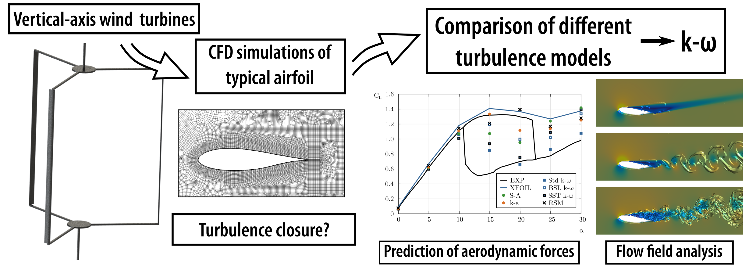
Turbulence-Model Comparison for Aerodynamic-Performance Prediction of a Typical Vertical-Axis Wind-Turbine Airfoil

by
Andrés Meana-Fernández
*,
Jesús Manuel Fernández Oro
,
Katia María Argüelles Díaz
and
Sandra Velarde-Suárez
Fluid Mechanics Area, Department of Energy, University of Oviedo, C/Wifredo Ricart s/n, 33204 Gijón, Spain
*
Author to whom correspondence should be addressed.
Energies 2019, 12(3), 488; https://doi.org/10.3390/en12030488
Submission received: 16 January 2019 / Revised: 30 January 2019 / Accepted: 31 January 2019 / Published: 2 February 2019
(This article belongs to the Section A3: Wind, Wave and Tidal Energy)

Abstract

:
In this work, different turbulence models were applied to predict the performance of a DU-06-W-200 airfoil, a typical choice for vertical-axis wind turbines (VAWT). A compromise between simulation time and results was sought, focusing on the prediction of aerodynamic forces and the developed flow field. Reynolds-averaged Navier–Stokes equation (U-RANS) models and Scale-Resolving Simulations (SRS), such as Scale-Adaptive Simulation (SAS) and Detached Eddy Simulation (DES), were tested, with k ω -based turbulence models providing the most accurate predictions of aerodynamic forces. A deeper study of three representative angles of attack (5 ° , 15 ° , and 25 ° ) showed that U-RANS models accurately predict aerodynamic forces with low computational costs. SRS modeling generates more realistic flow patterns: roll-up vortices, vortex packets, and stall cells have been identified, providing a richer unsteady flow-field description. The power spectrum density of velocity at 15 ° has confirmed a broadband spectrum in DES simulations, with a small peak at a Strouhal number of 0.486. Finally, indications regarding the selection of the turbulence model depending on the desired outcome (aerodynamic forces, airfoil flow field, or VAWT simulation) are provided, tending toward U-RANS models for the prediction of aerodynamic forces, and SRS models for flow-field study.

Graphical Abstract

1. Introduction

In a world context in which living without electricity is almost inconceivable, the development of renewable and sustainable energy sources is of vital importance. Wind energy represents a power source that is becoming cheaper and more competitive over time, being inexhaustible, renewable, and noncontaminant. Although research has traditionally focused on horizontal-axis wind turbines (HAWTs), vertical-axis wind turbines (VAWTs) have important advantages, the main one being that they are capable of working independently of the wind direction. They can produce energy from lower wind speeds, so they can be placed nearer to the ground, making installation and maintenance easier. The noise level generated by VAWTs is also lower. All these advantages make VAWTs especially suitable for installation in urban areas. On the other hand, VAWTs have some disadvantages that cannot be disregarded, the main ones being the difficulty to self-start and lower efficiency compared to HAWTs [1]. Due to the continuous changing of the relative position of the blades with respect to the incoming wind, flow behavior is much more complex, with the blades working even at stall conditions during part of the rotation cycle. Considering this particular characteristic, the importance of employing an optimized airfoil design for turbine blades is evident.
The shape of the airfoil used to build turbine blades determines the aerodynamic forces that are developed on their surface and, hence, the amount of energy that is extracted from the wind. In the case of lift-driven turbines, the aim is maximizing lift force (perpendicular to the incoming wind direction) and reducing drag force (in the direction of the incoming wind). For testing prospective airfoils, wind-tunnel experiments using a force balance are the most typical way of obtaining airfoil aerodynamic forces (lift, drag, and moment coefficients) as a function of incoming wind speed and angle of attack [2]. Nevertheless, the design of the experiments, the construction of airfoil prototypes, and the costs related to the reservation and use of experimental facilities require an amount of time and effort that some small companies and institutions cannot afford at the first stages of design. In these instances, Computational Fluid Dynamics (CFD) models become convenient to predict the behavior of a prospective airfoil shape before proceeding to more expensive experimental tests. There are many examples of the use of CFD codes for performance prediction of existing airfoils under steady conditions [3,4,5,6,7]. Sørensen et al. [8] compared seven CFD codes for 2D airfoil flows, proposing a series of suggestions for best practice. Athadkar and Desai [9] studied the appropriate position of boundary conditions for airfoil simulation. They found that at least a distance of 10c from the airfoil to the inlet and sides of the domain, and a distance of 15c to the domain outlet were necessary for the correct simulation of airfoil flows. Eleni et al. [10] compared three different turbulence models for the prediction of airfoil flows, highlighting the necessity for further research into turbulence modeling. CFD simulations have been useful for studying unsteady effects, such as dynamic stall produced by airfoil pitching or oscillations in incoming velocity [11,12,13]. In addition, flow particularities, such as modifications of fluid viscosity [14] or the influence of suspended sand in the aerodynamic performance of airfoils [15], are difficult to model with simpler codes. Regarding airfoil geometry, CFD simulations allow the study of different modifications just by modifying the geometry in the domain. Li et al. [16] studied the influence of airfoil trailing-edge thickness on performance. Mendez et al. [17] studied the effect caused by distributed roughness on the airfoil surface, whereas Schramm et al. [18] studied the influence of wind-turbine-blade erosion. Finally, Obeid et al. [19] simulated a NACA0015 flapped airfoil, whereas Fernandez-Gamiz et al. [20] simulated a series of Gurney flaps and microtabs, building afterwards a reduced-order method from the CFD results. Hence, CFD airfoil simulations are very useful for the performance prediction of different airfoils, allowing the introduction of multiple effects that are typically neglected in lower-order methods. This is of particular interest for the design of optimized airfoils [21,22].
In this work, different turbulence models were applied to predict the performance of a particular airfoil, the DU-06-W-200 [23]. The main aim of this study was to find a compromise between simulation time and results, and not just to focus on the prediction of airfoil aerodynamic forces, but also o provide insight into the flow field developed around and downstream from the airfoil. This is of particular interest concerning the application to vertical-axis wind turbines, as an accurate description of vortex shedding from the blades at the upwind part of the turbine would be very useful to obtain realistic flow incoming conditions for the downwind part of the turbine. Reynolds Averaged Navier–Stokes equation (U-RANS) models, which apply phase-averaging to the Navier–Stokes equations to model the turbulent part of the flow, offer the most economic approach for computing complex turbulent industrial flows [24]. They are suitable for many engineering applications and typically provide the required level of accuracy. An alternative to these models are Scale-Resolving Simulation (SRS) models, which resolve at least a portion of the turbulence for at least a portion of the fluid domain (typically, larger and more problematic scales), leaving the turbulence model to account for just the effects of more universal and smaller isotropic scales [24]. This family includes Direct Numerical Simulations (DNS), which solve flow scales up to the Kolmogorov scale; Large Eddy Simulations (LES), which solve the largest flow scales; and hybrid LES-RANS models, like Scale-Adaptive Simulation (SAS) models, Detached Eddy Simulation (DES) models, and Embedded LES (ELES) models, which combine elements of LES and RANS approaches to allow the simulation of high Reynolds flows, avoiding the high-resolution LES requirements. Regarding the scope of this work, it was intended to go further than the application of U-RANS models and include SRS. Finally, we obtained from our results some indications regarding turbulence-model selection, depending on the desired outcome (airfoil aerodynamic forces, airfoil flow field, or VAWT simulation). More specifically, k ω turbulence models provide the most accurate results, with U-RANS schemes being helpful to obtain quick predictions of aerodynamic forces. The SAS and DES approaches, on the other hand, provide a richer description of the flow field with unsteady structures, being suitable to model the flow that reaches the downwind part of a VAWT.

2. Numerical Methodology

2.1. Experimental Reference Case

An experimental reference case was used to validate numerical simulations. The experimental data were obtained at the Low Turbulence Tunnel (LTT) from the Technical University of Delft [23]. This tunnel has a test section of 1.8 times 1.25 m (width × length), and a turbulence level of 0.02%. The tested airfoil had a DU-06-W-200 section with a chord of 0.25 m. This airfoil was specifically designed for vertical-axis wind-turbine applications, and it was claimed that it has the ability to self-start the turbine. The Reynolds number used for the tests was 300,000, corresponding to an incoming flow velocity of approximately 17 m/s.

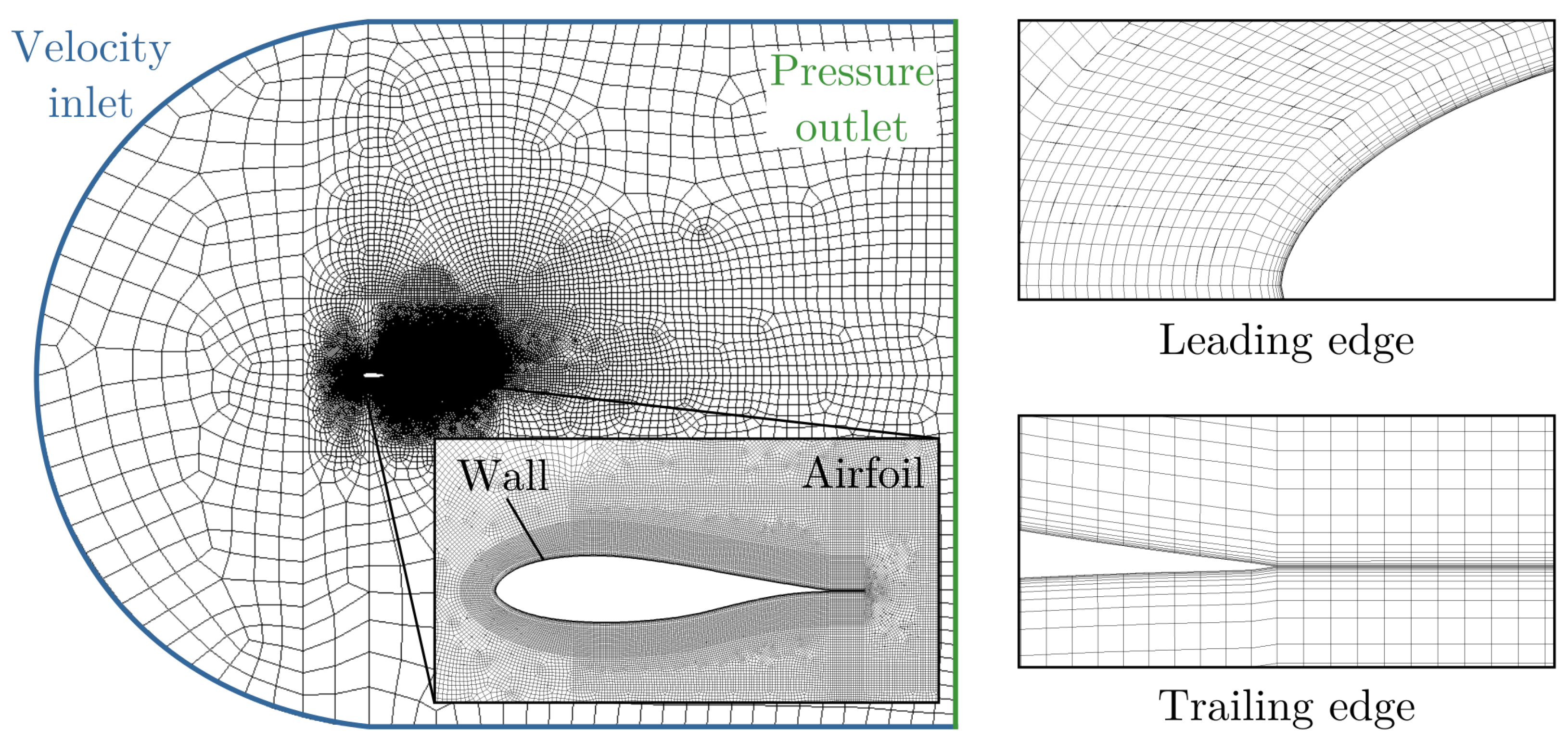
2.2. Domain Geometry and Proper Mesh-Size Study

In order to select a proper domain size, a literature survey was performed. Table 1 shows a selection of typical domain sizes found in the literature in airfoil chord units c for airfoil simulation. In the comparative benchmark developed by Sørensen et al., Mendez and Muñoz from the CENER Research Center demonstrated that a domain size of 25c× 25c was enough to obtain accurate results [8]. For the case to be simulated in this work, a distance to the inlet of 12.5c and a distance to the outlet of 20c (domain size 32.5c× 25c), in line with typical values found in the literature, were considered enough to avoid the effect of the boundaries on the development of the flow inside the domain region. Figure 1 shows the final employed domain for the simulation, alongside the mesh and the applied boundary conditions.
The initial aim of this work was to compare wall-resolved and wall-modeled turbulent schemes, so two different grids with different requirements were generated using GAMBIT® software. For grid-size calculation, displacement thickness δ * of the airfoil boundary layer at a medium angle of attack (15 ° ) was estimated using XFOIL [25] software. At a Reynolds number of 300,000, this size was estimated to be around 25 mm (sum of the pressure and suction side values). As boundary-layer thickness δ was larger than δ * , and the largest scales in a boundary layer are of a typical size L δ / 2 to δ / 8 , it may be assumed that L is approximately of the same size as the displacement thickness calculated with XFOIL. Following the recommendations of Davidson and Dahlström, the largest scales in a boundary layer are in the order of δ , and these scales are probably also apparent in the spanwise direction [26,27]; thus, ratio δ / L z should at least be less than one, L z being the spanwise extent of the domain. Hence, L z was chosen to be 25 mm, twice the estimated displacement thickness, resulting in a ratio between the spanwise extent of the domain ( L z / c = 0.1 ), higher than the one reported in Reference [26].
Regarding the number of nodes in the spanwise direction, the guidelines proposed in References [24,28] were followed. As there are different mesh requirements depending on whether the flow near the walls is to be resolved (wall-resolved LES resolution, WRLES) or modeled (wall-modeled LES resolution, WMLES), two different meshes were generated. In order to obtain a wall-resolved LES resolution, a dimensionless wall distance Δ z + 10 to 40 is recommended. Taking 20 as a reasonable value, cell size would be 0.75 mm, which results in 33 cells inside the boundary layer. For a wall-modeled LES resolution, it is enough with Δ z + values between 100 and 300 (a cell size of around 3.75 mm, resulting in 7 cells inside the boundary layer). On the other hand, following the recommendation from Reference [28], 20 cells are recommended inside the boundary layer, resulting in a typical cell size of 1.25 mm, which was the value finally adopted.
Concerning the in-plane mesh requirements [27], recommendations are Δ x + = 50 to 150 and Δ y + = 20 to 150 for wall-modeled LES resolution. For a wall-resolved LES resolution, the values are Δ x + = 50 to 150 and Δ y + = 1 . These requirements result in typical cell sizes of 11 and 1.5 mm in the x-direction for wall-modeled and wall-resolved LES, respectively, and 0.75 and 0.04 mm in the y-direction. These values are aligned with the value proposed by Reference [28], Δ x δ / 10 = 2.5 mm.
Additionally, the total number of cells recommended in the volume region inside the boundary layer are scaled with the Reynolds number of the flow [24] with the following formulas:
  • For the outer-layer region ( y + 100 to δ + 1360 ):
    N Ω = 3000 × ( w / c ) × R e 0.4
  • For the inner-layer region ( y + 0 to y + 100 ):
    N Ω = 5 × 10 4 × ( w / c ) × R e 1.8
R e being the flow Reynolds number, w the spanwise extent of the domain, and c the airfoil chord. Additionally, it is advisable to have between three and five cells in the region below y + 10 . Following all of these recommendations, the values of Δ y 2.5 mm and Δ y 0.027 mm were adopted for the outer and inner layer, respectively.
Finally, the total number of cells in the outer region of the boundary layer ( y + 100 to δ + 1360 ) was set according to the typical cell size calculated for wall-modeled LES requirements ( 1.5 mm in the streamwise direction and 2.5 mm in the spanwise direction). These values are consistent with the values proposed by Chapman [29,30], who proposed a value of Δ c e l l δ / N 1 / 3 1.9 mm, and Pope [28], who proposed Δ c e l l = π / κ c 2 mm, κ c 38 / L being the frequency of the LES filter that accounts for 80% of turbulent kinetic energy.
Following all these guidelines, wall-modeled and wall-resolved LES meshes resulted in 1,640,394 and 4,328,775 cells, respectively. Figure 1 shows the final mesh for the wall-modeled simulations, with details of the mesh near the leading and the trailing edge of the airfoil. Previous studies from the authors for the simulation of a complete turbine using the Richardson extrapolation method to assess mesh convergence showed that a mesh discretization of 40 cells in the first 2 mm from the airfoil wall in the cross-stream direction, and 12 cells/mm in the streamwise direction of the airfoil chord, were enough to capture all relevant fluid phenomena. Therefore, the mesh used in this work, even finer and used for the analysis of a static airfoil, may be considered fine enough (apart from having been prepared following all the recommendations in the literature for this kind of simulations). The mesh had a maximum aspect ratio of 220 (in the boundary layer), a minimum orthogonality of 0.42 (where 0 and 1 represent low and high quality values, respectively), and a maximum skewness of 0.58 (where 0 and 1 represent high- and low-quality values, respectively).

2.3. Numerical Solver, Boundary Conditions, and Turbulence Models

The Navier–Stokes equations were solved in an incompressible fashion using commercial software ANSYS-FLUENT®. The boundary conditions of the simulation domain are shown in Figure 1 alongside the mesh. A velocity-inlet condition was set at the domain inlet with a value of 17 m/s that corresponds to a Reynolds number of 300,000. At the domain outlet, a pressure-outlet condition equal to atmospheric pressure was set. The airfoil was defined with the wall-boundary condition (no-slip), and the spanwise limits of the domain were set as a symmetry boundary condition.
To calculate the turbulence values at the inlet, knowing wind-tunnel turbulence intensity ( I = 0.02 % ), the typical length scale of the tunnel was estimated as [24]:
= 0.07 L C μ 3 / 4 = 0.767 m
where L = 1.8 m is the characteristic length of the wind tunnel, and C μ = 0.09 is a constant used to ensure consistency with the definition of turbulent length scales. With these two values, turbulent kinetic energy at the inlet is calculated as:
k = 3 2 ( u ¯ I ) 2 = 1.743 × 10 5 m 2 / s 2
where u ¯ is the mean flow velocity. Then, depending on the turbulence model, the corresponding turbulent variables may be calculated as:
  • Modified turbulent viscosity:
    ν ˜ = C μ 3 2 u ¯ I = 2.874 × 10 4 m 2 / s
  • Turbulent dissipation rate:
    ε = k 3 / 2 = 9.492 × 10 8 m 2 / s 3
  • Specific dissipation rate:
    ω = k 1 / 2 C μ = 0.0605 s 1
The tested U-RANS turbulence models in this study are the following:
  • (1) Strain-based Spalart-Allmaras;
  • (2) Realizable k ε with Enhanced Wall Treatment;
  • (3) k ω (Standard, Baseline, and Shear-Stress Transport [31]); and
  • (4) Linear Pressure-Strain Reynolds Stress model with Enhanced Wall Treatment.
The studied SRS models are:
  • (1) SAS with k ω Standard and Shear Stress Transport models;
  • (2) WMLES Standard and WMLES S Ω ;
  • (3) LES with the Wall-Adapting Local Eddy-Viscosity (WALE) model; and
  • (4) Detached Eddy Simulation with the k ω Shear Stress Transport model.
Additionally, XFOIL, an interactive program for the design and analysis of subsonic isolated airfoils [25], was employed to calculate airfoil aerodynamic forces with a complementary method.
Due to the variety of turbulence models, several discretization schemes were employed. The SIMPLE algorithm was used for the pressure–velocity coupling for all studied cases. Spatial discretization regarding gradient terms was selected to be the Least-Squares Cell-Based discretization. The rest of the spatial discretization schemes (pressure, momentum, turbulent quantities) were chosen to be at least of second order for all cases. Finally, regarding transient formulation, Second-Order Implicit formulation was chosen for the U-RANS models, whereas the Bounded Second-Order Implicit was used for the SRS models.

2.4. Time-Step Selection and Calculation Time

Time-step selection for the simulations depends on the chosen turbulence model. For U-RANS models, it was assumed that only the fluctuations associated with vortex shedding are captured, related to a value of 0.2 for the Strouhal number [32] based on blade chord c and bulk velocity u ¯ , thus corresponding to a vortex-shedding period of:
T s h = c 0.2 × u ¯ = 0.073 s
Assuming that at least 25 time steps per cycle are required to capture those fluctuations, the time step for the U-RANS simulations was chosen as Δ t U R A N S 2.5 × 10 3 . For SAS models, as higher fluctuation levels are expected, this time step was set to be one order of magnitude less than for U-RANS simulations, 2.5 × 10 4 s. This value lies between the value set for the U-RANS and for the LES simulations (not as many fluctuations as for the LES models are expected).
For wall-modeled Large Eddy Simulations, aiming at resolving around 80% of the turbulent kinetic energy of the flow [28], κ c L 38 with κ c 2 π / c , so that c / L 0.16 . Applying the concept of the energy cascade ( u c 3 / c U 3 / L ) that relates the scales and velocities of the greater vortices (L, U) and the vortices corresponding to the cut-off frequency of the LES filter ( c , u c ), it is possible to determine the time step for the WMLES simulation: Δ t W M L E S 1 25 c u c 1 25 c U ( c / L ) 1 / 3 1 25 0.16 L U ( 0.16 ) 1 / 3 = 0.16 2 / 3 25 L U . Assuming that L δ 25 mm and U 1.7 m/s, one order of magnitude less than the mean flow velocity, the time step required for the wall-modeled Large Eddy Simulations simulations is Δ t W M L E S 1.75 × 10 4 s.
Finally, for wall-resolved Large Eddy Simulations, the time step may be calculated as the ratio between the smallest cell size and fluctuating velocity U. Assuming y + 1 , the required time step is: Δ t L E S Δ y U 3.5 × 10 5 1.7 2 × 10 5 s. Table 2 outlines the time-step sizes selected for each family of turbulence models.
The flow was simulated at the following angles of attack: 0 ° , 5 ° , 10 ° , 15 ° , 20 ° , 25 ° and 30 ° . Simulations were performed using a four-node Intel Core i7-52820K at 3.3 G H z and 64 G b RAM, with the simulation time depending on the chosen turbulence model, as stated in Table 2.

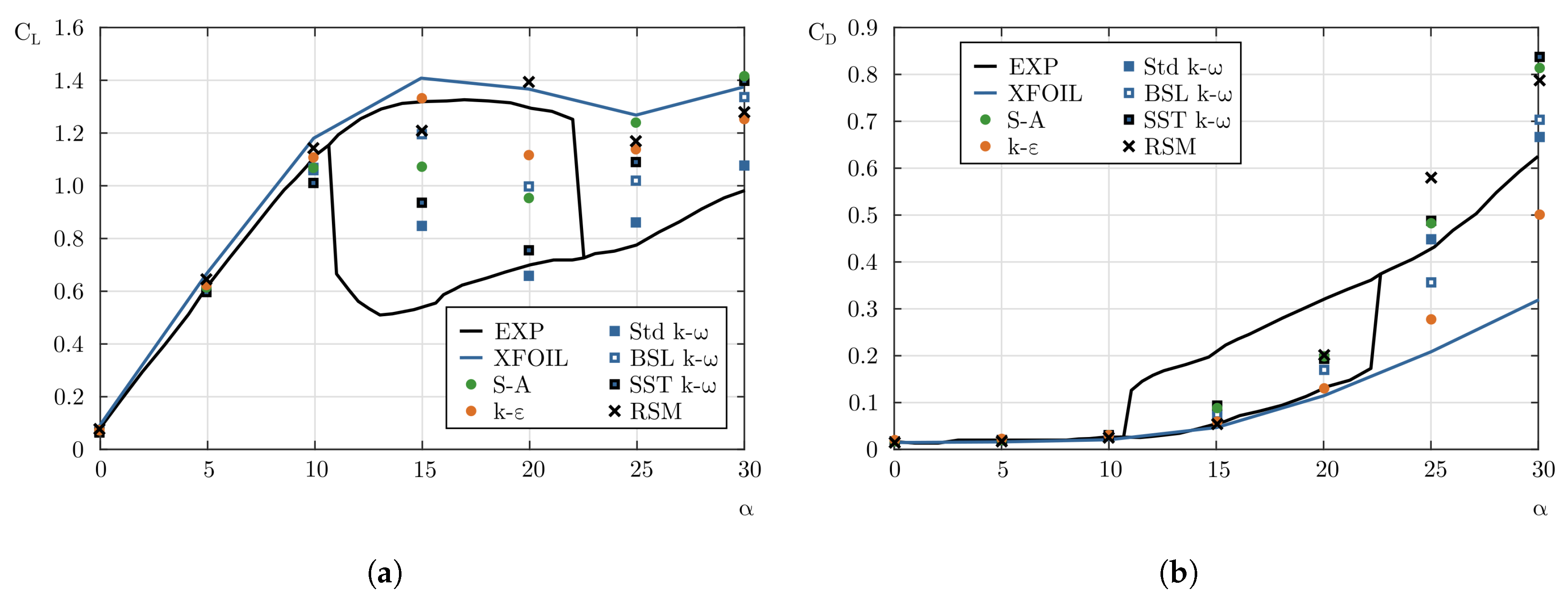
3. Prediction of Aerodynamic Forces on Airfoil

3.1. U-RANS Simulation Results

Figure 2 shows the experiment results from the wind tunnel (black line) alongside XFOIL predictions (blue line) and the different U-RANS models tested in this study. It may be observed that the XFOIL predictions are quite accurate before the stall angle, as already known from the literature [25]. The experiment results present a characteristic hysteresis loop, typically found in airfoils at high angles of attack at low Reynolds numbers, and related to the stall behavior of the airfoil and the possible formation of a laminar separation bubble [33]. Regarding CFD models, both the Spalart-Allmaras (S-A) and k-epsilon ( k ε ) models fail to accurately predict the airfoil aerodynamic forces. The S-A model overpredicts both lift and drag, whereas the k ε model overpredicts lift but underpredicts drag, artificially increasing the performance of the airfoil. The employed Reynolds stress model, besides requiring more computational effort (five additional equations), did not yield better results. The best results were obtained with the k ω models, which were found to be well-adapted to low Reynolds flows with adverse pressure gradients [34]. More specifically, the Standard (Std) and Shear Stress Transport (SST) models seemed to provide the best results. For these reasons, those two models were selected to perform Scale-Resolving Simulations (Scale-Adaptive Simulations and Detached Eddy Simulations), and provide more insight into flow details around the airfoil.

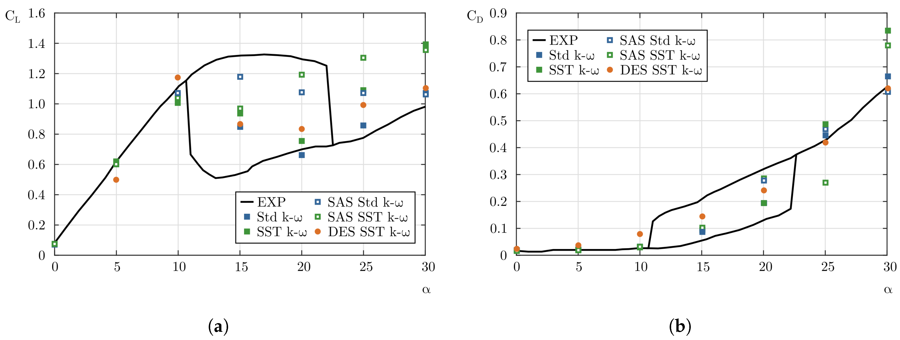
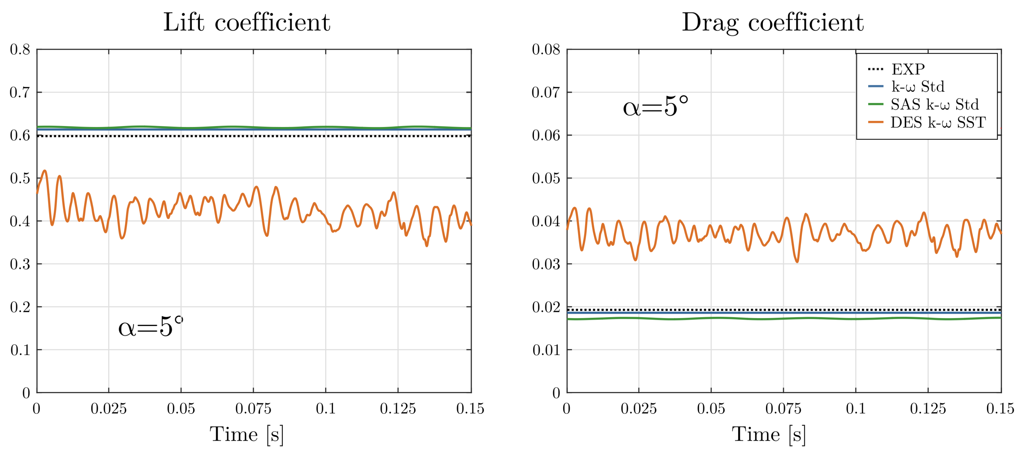
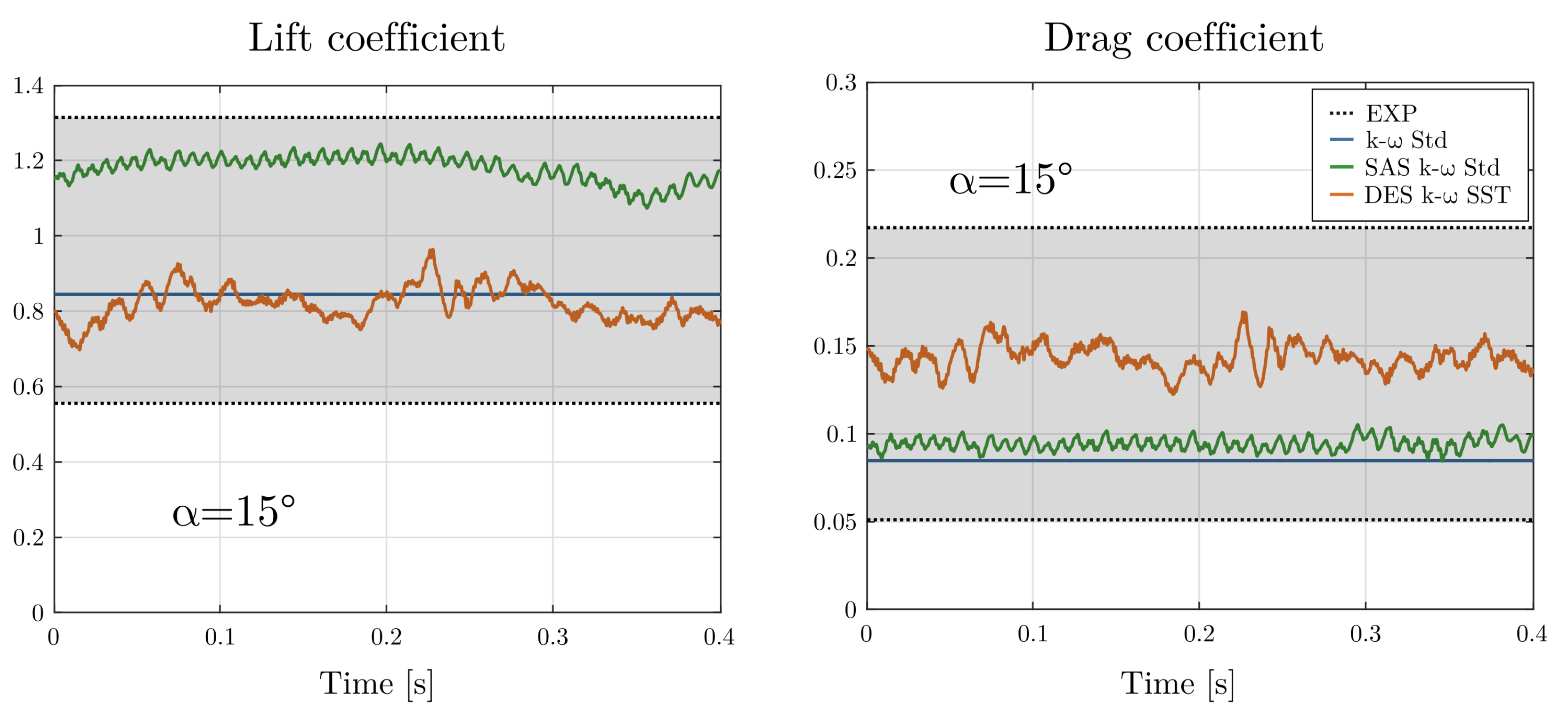
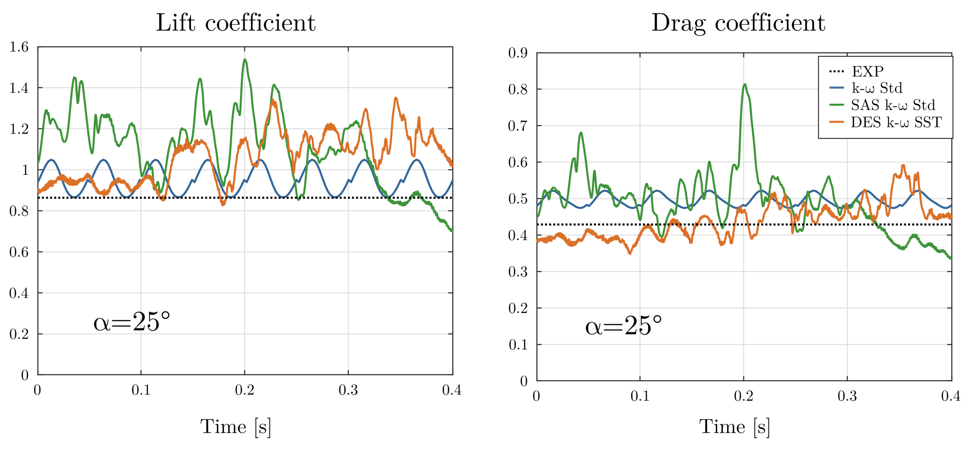
3.2. Results from the SRS Simulations

Figure 3 shows the aerodynamic force predictions of the selected U-RANS models ( k ω Standard and SST) alongside the SRS models based on those U-RANS models (SAS and DES). Regarding the prediction of the airfoil aerodynamic forces, the k ω Standard (U-RANS) is the most accurate model. The formulations based on the SST model are not so accurate in the U-RANS and SAS cases, especially at higher angles of attack. On the other hand, the DES formulation seems to predict reasonably well the forces at high angles of attack after the stall angle. Thus, the models that seem more suitable for the prediction of airfoil aerodynamic forces are the U-RANS k ω Standard, the SAS (with k ω Standard formulation) and the DES (with k ω SST formulation), being the U-RANS k ω Standard model the best recommendation if the only objective of the study is the prediction of the aerodynamic forces for an airfoil (insight into the flow field will be later discussed).
With the aim of investigating the causes of the differences in predicted values between the three selected models, Figure 4, Figure 5 and Figure 6 were added showing the temporal evolution of the lift and drag coefficients for three angles of attack: 5 ° (low), 15 ° (medium), and 25 ° (high). The experimental values are time-averaged; they are represented with dashed lines in the figures.
Regarding the predicted values at 5 ° (low angle of attack, Figure 4), both the U-RANS and the SAS models predict values very close to the experimental values, whereas the DES model tends to slightly underpredict lift and overpredict drag. This could be explained by the small size of the boundary layer, still too attached to the airfoil, that could activate the LES filter of the DES modeling, affecting the U-RANS solution. In other words, it is not recommended to employ SRS models for the description of nondetached flows in case of relatively coarse grids with respect to boundary layer size.
At a medium angle of attack (15 ° , Figure 5), experimental values oscillate between a maximum and a minimum value (the result of the hysteresis loop related to stall, previously commented). All turbulence models predict values between these experimental values (gray zone in Figure 5), so it is not easy to determine which of the models is the most suitable. The U-RANS and DES models predict similar lift values, with SAS formulation predicting higher values, whereas, for the drag prediction, DES formulation is the one predicting higher values, with the U-RANS and SAS models predicting almost the same value. Figure 7, which shows the pressure coefficient on the airfoil at this angle of attack (15 ° ), was added to highlight the mechanisms behind the discrepancies between the values predicted by the three different models. The area enclosed by the pressure-coefficient curve of the SAS model is substantially bigger than for the other two models according to the higher lift values predicted by this model. On the other hand, the parts of the curves on the suction side are very similar for the three models. No specific recommendations can be provided regarding intermediate angles of attack.
Finally, at a high angle of attack (25 ° , Figure 6), there is high instability in lift and drag values for the SRS models. The value fluctuations of the forces are also present in the U-RANS model. The three models oscillate around a mean value, the U-RANS model again being the one that yields values more similar to the experiment ones. In this case, the DES model performed better than the SAS model, which slightly overpredicted the values of both aerodynamic forces. This poststall situation of the airfoil, with a fully detached wake, might benefit from the turbulent description of the DES model.

3.3. Additional Remarks

The mesh requirements for performing WMLES and LES simulations ([24,26,27]) were carefully followed. Despite the mesh, the obtained results were not substantially better than the results from other turbulence models. Presumably, the mixing-length model employed near the wall for the WMLES model is too simple compared to the other employed turbulence models, being unable to correctly model the adverse pressure gradient that develops on the airfoil surface. In the pure LES case, however, the reason behind the model performance is likely the need for mesh refinement near the airfoil wall. Since both WMLES and LES simulations were already much more time-consuming than the other ones, further mesh refinement would lead to extremely long computational times, far beyond the required balance between simulation time and accuracy for the present research.

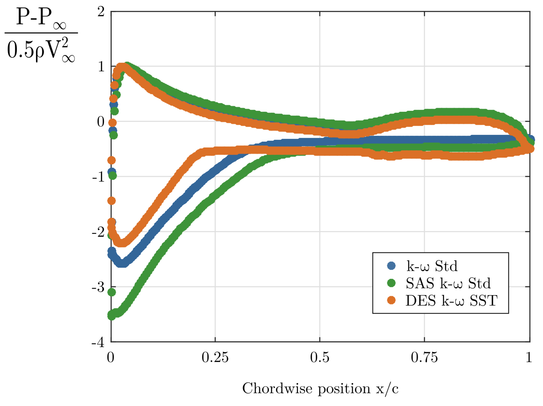
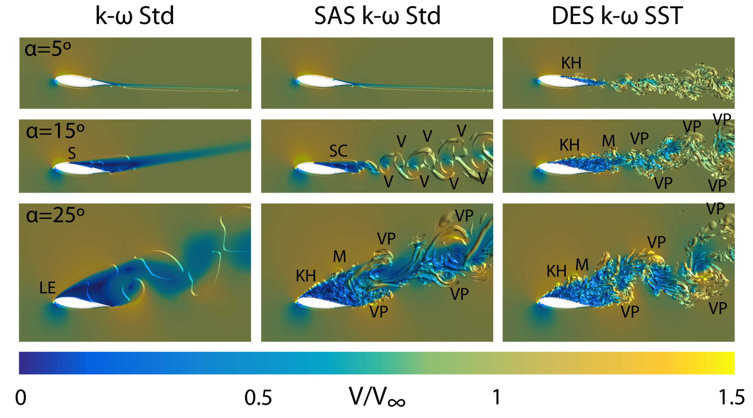
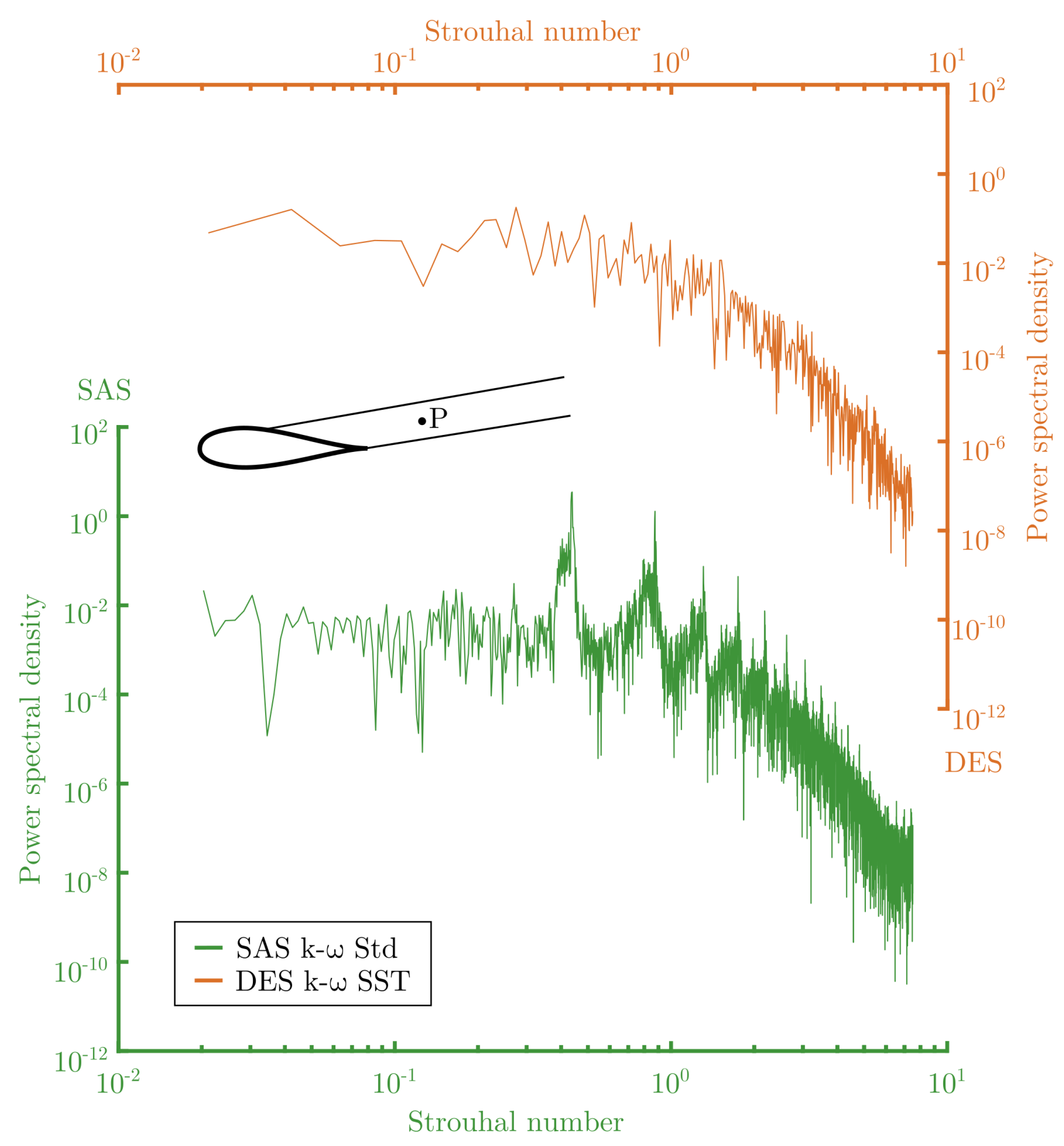
4. Flow-Field Analysis

After discussing the prediction results of aerodynamic forces on the airfoil, the results for flow-field prediction around the airfoil are discussed in this section.
Figure 8 shows the contours of the instantaneous normalized velocity field around the airfoil for the three models selected in the previous section of this study: U-RANS k ω Standard, SAS k ω Standard, and DES k ω SST, and the three angles of attack detailed before: 5 ° , 15 ° , and 25 ° . On top of the contours, isosurfaces of Q-criterion = 50 s 2 were added to make the identification of vortical structures easier. The Q-criterion method, the most widely used in LES-based simulations [35], defines a vortex as a spatial region where the Euclidean norm of vorticity tensor Ω i j dominates that of rate of strain S i j : Q = 1 2 | Ω i j Ω i j | 2 | S i j S i j | 2 > 0 .
The differences in flow-field prediction between the different models are quite apparent. The k ω Standard model shows a clean flow pattern at all studied angles of attack, with big blobs of Q isovalues being convected by the incoming wind flow. The SAS k ω Standard approach allows to break up these large structures into smaller scales. This approach leaves the U-RANS part of the model unaffected by grid spacing, so it does not allow model-accuracy deterioration in regions of refined grid but insufficient flow instability (this behavior was observed in DES models and could explain the results commented before for α = 5 ° ). However, in cases where flow instability is not strong enough, the SAS remains in U-RANS mode and does not produce unsteady structures (as seen precisely for α = 5 ° in Figure 8) [24]. DES k ω SST formulation produces unsteady structures for all angles of attack, yielding a more realistic flow pattern behind the airfoil according to typical patterns observed in the literature for airfoils at low Reynolds numbers ([36]). Some roll-up vortices caused by Kelvin-Helmholtz instabilities in the shear layer may be identified (marked as KH in Figure 8), and a small wake with not very organized structures becomes apparent, as in the work of Yarusevych et al. [37].
With the increase of the angle of attack, the widening of the wake and vortex-shedding phenomena become apparent. The separation of the shear layer (S) and the development of a stall cell (SC), also found in the work of Sarlak et al. [33], are detectable with the three employed turbulence models. Additionally, at α = 15 ° , flow instability is strong enough for SAS formulation to produce unsteady structures. A coherent vortex-shedding pattern, similar to a von Karman vortex street, appears downstream from the airfoil in a clearly organized pattern (the identified vortices are marked as V in Figure 8). Nevertheless, DES formulation shows a more intricate pattern, in which the periodicity of the shedding phenomena is not so clearly visible, but is clearly more realistic according to the bibliography [36,37,38]. Kelvin-Helmholtz instabilities arise in the shear layer, generating roll-up vortices (KH) that eventually merge (M), then break down into smaller scales and accumulate into larger structures, forming packets. These vortex packets (VPs), such as the ones found by Rodríguez et al. [38], are present, but their pattern is not so clear, suggesting broadband frequency-centered activity, similar to the one found by Yarusevych et al. [37]. This is related to weaker and less-coherent structures that could be generated by the separation of a bubble from the airfoil surface [33], which could explain the static-stall hysteresis behavior found in this airfoil. Finally, for the highest angle of attack, α = 25 ° , the wake was so wide and unsteady that even the U-RANS k ω Standard was able to capture the vortex-shedding blobs in the flow as they were convected downstream. Separation already occurs at the airfoil leading edge (LE) for the three turbulence models. Roll-up vortices in the shear layer related to Kelvin–Helmholtz instabilities (KH) and their merging (M) are captured by both SAS and DES models, and VPs are easily identifiable. In this case, shifting toward more scale-resolving models, such as SAS or DES, substantially increases the richness of the flow description (and, as previously confirmed, with no harsh effect on aerodynamic-force prediction on the airfoil).
Lastly, the Power Spectrum Density (PSD) of the instantaneous velocity signal was computed at a point placed in the middle of the airfoil wake at α = 15 ° , 0.24c downstream the airfoil. Figure 9 shows the results for the two scale-resolving models (SAS k ω Std and DES k ω SST) as a function of the Strouhal number, providing more insight into the pictures in the middle row of Figure 8. The results from the RANS model are not shown as the magnitude of the fluctuations captured was not significant, in agreement with the flow field depicted in Figure 8. The Strouhal numbers were calculated with the projection of the airfoil chord in the cross-streamwise direction and incoming flow velocity as S t = f c sin ( α ) / u ¯ , where f is each corresponding frequency and c is the chord. With the scale-resolving models, higher frequencies may be captured and energy is no longer concentrated in large scales, as they are then able to break up. In SAS modeling, the peak in the spectrum is produced at a S t = 0.438 . The clear peaks of the spectrum are related to the clean vortex street that is apparent in Figure 8. On the other hand, regarding DES simulations, the spectrum was smoother, with a small peak at S t = 0.486 , the same Strouhal number as for the SAS simulations. Another peak at around half of that value, S t = 0.233 , was also apparent in the spectrum, and may be related to the subharmonic frequency due to the merging of the roll-up vortices from the shear layer. This subharmonic peak was also observed in previous research ([37,38]). Finally, broadband frequency-centered activity was visible in the spectrum, related to the low-frequency oscillation mechanism reported at near-stall angles by Rodríguez et al. [38]. DES modeling allows a more realistic break up of the large eddies and the capture of this broadband-frequency activity, which may explain the sea of vortices found in Figure 8, although some periodicity may be deduced from deeper analysis of the figure.
From previous analyses of this study, it is clear that the turbulence model should be adjusted depending on the desired simulation outcome. The U-RANS model used in this study is able, at a very low computational cost (3% of the simulation time of a SAS), to accurately predict the aerodynamic forces on an airfoil. So, if the only aim were to predict the forces on an airfoil, it would make sense to only perform a U-RANS simulation using the k ω model for turbulence closure. However, if the aim were to characterize the flow field behind the airfoil, an SAS formulation at least should be employed, and a DES formulation would be advisable to obtain information about the smallest scales of the flow (always being careful with the grid in cases of not enough flow instability). Additionally, in the case of airfoils suffering from hysteresis loops in aerodynamic forces, special attention should be paid to the turbulence model in order to accurately capture the separation of the boundary layer from the airfoil.
Nevertheless, these conclusions should not straightforwardly be extrapolated to airfoils working as part of a vertical-axis wind turbine. Even if it were desired to only predict the forces on turbine blades (and, thus, a U-RANS model would be the best option in terms of accuracy/cost), when the blades pass by the downstream half of the turbine, it is unlikely that they find the flow conditions shown in Figure 8, left. Indeed, a correct description of the downstream flow from the airfoils passing by the upwind half of the turbine, such as that provided by a DES model, could prove itself useful as part of a better prediction of incoming flow conditions in the downstream part of the turbine. In addition, the flow field developed by the turbine strongly depends on the ratio between its rotational speed and the incoming wind speed, leading to different flow patterns, with more or less detached flow from the airfoils. Thus, it could be wise to apply SRS models with high-resolution capabilities when the rotational velocity of the turbine is slow compared with the incoming wind speed to correctly resolve the detached flow field that arises. On the other hand, turbines with higher rotational speeds will present more attached boundary layers and smaller eddy sizes. In these cases, a U-RANS model could be able to describe the flow field with relatively enough accuracy while substantially reducing the required computational resources.

5. Conclusions

In this work, different turbulence models were applied to predict the performance of a particular VAWT airfoil. The best results between the U-RANS models were obtained with the k ω turbulence models, with k ε and S-A overpredicting airfoil performance. Reynolds stress models required more computational effort and did not produce better results. These conclusions are in line with the literature, as k ω models have been found to be well-adapted to low-Reynolds flows with adverse pressure gradients. Regarding SRS simulations, both k ω -based SAS and DES models predict the aerodynamic forces with relatively good accuracy, also resolving the flow scales that arise with detached flow conditions. The temporal evolution of lift and drag coefficients for three angles of attack (low—5 ° , medium—15 ° , and high—25 ° ) was studied in depth, finding that the small size of the boundary layer at low angles of attack may lead to inaccurate results in SRS simulations due to artificial activation of the LES filter. Concerning intermediate angles of attack, U-RANS, SAS, and DES models oscillate around a mean value, all of them inside the region, determined by maximum and minimum experimental values. The area enclosed by the pressure coefficient curve of the SAS model was substantially bigger, predicting higher lift values. Further research should be performed at intermediate angles of attack. Finally, at the highest angle of attack, although the U-RANS model provides results more similar to the experiments, the poststall situation of the airfoil benefits from the turbulent description of the DES model.
Results from flow-field analysis showed that the most realistic flow patterns, according to the literature, are the ones obtained with DES modeling. Roll-up vortices caused by Kelvin–Helmholtz instabilities that subsequently merge into vortex packets were identified, as well as the stall cell associated with the lift decrease of the airfoil. DES models showed a more intricate pattern, suggesting broadband frequency-centered activity, related to weaker and less coherent structures that could be generated by a separation bubble. Analysis of power-spectrum density of the velocity signal at α = 5 ° confirmed this broadband spectrum in DES simulations, with a small peak at a Strouhal number equal to 0.486. In SAS modeling, an apparent peak appears at 0.438, related to the clean vortex streets that arise as a consequence of choosing this turbulence model.
In conclusion, U-RANS models are able (with only 3% of the computational cost of a SAS), to accurately predict aerodynamic forces on the airfoil. On the other hand, SAS or DES formulations are advisable to obtain information about the smallest flow scales. In addition, in the case of hysteresis loops in the aerodynamic forces, special attention should be paid to the turbulence model to accurately capture the separation of the boundary layer from the airfoil.
Finally, in the case of airfoils working as part of a vertical-axis wind turbine, these conclusions do not directly extrapolate. The flow field at the downstream half of the turbine is affected by the flow detached from the airfoils at the upwind half, so a correct description of the flow downstream the airfoils, such as that provided by SRS models, seems more meaningful than a U-RANS model. In addition, as the flow field developed by the turbine strongly depends on the ratio between its rotational speed and incoming wind velocity, employing U-RANS or SRS formulations, depending on expected flow conditions, would provide the best ratio between result quality and computational cost.

Author Contributions

Conceptualization, J.M.F.O.; formal analysis, A.M.-F. and J.M.F.O.; funding acquisition, K.M.A.D. and S.V.-S.; investigation, A.M.-F.; methodology, A.M.-F., J.M.F.O., K.M.A.D. and S.V.-S.; resources, K.M.A.D. and S.V.-S.; supervision, J.M.F.O., K.M.A.D. and S.V.-S.; writing—original draft, A.M.-F.; writing—review and editing, A.M.-F., J.M.F.O., K.M.A.D. and S.V.-S.

Funding

This work was supported by Project “Desarrollo y construcción de turbinas eólicas de eje vertical para entornos urbanos” (ENE2017-89965-P) from the Spanish Ministry of Economy and Business, the “FPU” predoctoral research scholarship provided by the Spanish Ministry of Education and Professional Training, and Projects “Desarrollo de una herramienta de diseño optimizado de perfiles aerodinámicos para su utilización en turbinas eólicas de eje vertical” from the University Institute of Industrial Technology of Asturias, financed by the City Council of Gijón, Spain, and “Diseño optimizado de una turbina eólica de eje vertical” from the University of Oviedo Foundation, financed by AST Ingeniería.

Conflicts of Interest

The authors declare no conflict of interest.

References

  1. Manwell, J.; McGowan, J.; Rogers, A. Wind Energy Explained: Theory, Design and Application; John Wiley and Sons, Ltd.: Chichester, UK, 2009. [Google Scholar]
  2. Tropea, C.; Yarin, A.; Foss, J. Handbook of Experimental Fluid Mechanics; Springer: Berlin, Germany, 2007. [Google Scholar]
  3. Cao, H. Aerodynamics Analysis of Small Horizontal Axis Wind Turbine Blades by Using 2D and 3D CFD Modelling. Master’s Thesis, University of Central Lancashire, Preston, UK, 2011. [Google Scholar]
  4. Sanz, J.M. CFD Study of Thick Flatback Airfoils Using OpenFOAM. Master’s Thesis, Technical University of Denmark, Copenhagen, Denmark, 2011. [Google Scholar]
  5. Yao, J.; Yuan, W.; Wang, J.; Xie, J.; Zhou, H.; Peng, M.; Sun, Y. Numerical simulation of aerodynamic performance for two dimensional wind turbine airfoils. Procedia Eng. 2012, 31, 80–86. [Google Scholar] [CrossRef]
  6. Rahimi, H.; Medjroubi, W.; Stoevesandt, B.; Peinke, J. 2D Numerical Investigation of the Laminar and Turbulent Flow Over Different Airfoils Using OpenFoam. J. Phys. Conf. Ser. 2014, 555, 012070. [Google Scholar] [CrossRef]
  7. Shah, H.; Mathew, S.; Lim, C. Numerical simulation of flow over an airfoil for small wind turbines using the γ-Reθ model. Int. J. Energy Environ. Eng. 2015, 6, 419–429. [Google Scholar] [CrossRef]
  8. Sørensen, N.; Méndez, B.; Noz, A.M.; Sieros, G.; Jost, E.; Lutz, T.; Papadakis, G.; Voutsinas, S.; Barakos, G.; Colonia, S.; et al. CFD code comparison for 2D airfoil flows. J. Phys. Conf. Ser. 2016, 753, 082019. [Google Scholar] [CrossRef]
  9. Athadkar, M.; Desai, S. Importance of the extent of far-field boundaries and of the grid topology in the CFD simulation of external flows. Int. J. Mech. Prod. Eng. 2014, 2, 69–72. [Google Scholar]
  10. Eleni, D.; Athanasios, T.; Dionissios, M. Evaluation of the turbulence models for the simulation of the flow over a National Advisory Committee for Aeronautics (NACA) 0012 airfoil. J. Mech. Eng. Res. 2012, 4, 100–111. [Google Scholar]
  11. Kasibhotla, V.; Tafti, D. Large eddy simulation of the flow past pitching NACA0012 airfoil at 1e5 Reynolds number. In Proceedings of the ASME 2014 4th Joint US-European Fluids Engineering Division Summer Meeting, Chicago, IL, USA, 3–7 August 2014. [Google Scholar]
  12. Li, S.; Zhang, L.; Yang, K.; Xu, J.; Li, X. Aerodynamic Performance ofWind Turbine Airfoil DU 91-W2-250 under Dynamic Stall. Appl. Sci. 2018, 8, 1111. [Google Scholar] [CrossRef]
  13. Zhu, C.; Wang, T. Comparative Study of Dynamic Stall under Pitch Oscillation and Oscillating Freestream on Wind Turbine Airfoil and Blade. Appl. Sci. 2018, 8, 1242. [Google Scholar] [CrossRef]
  14. Hawley, J. An OpenFoam Analysis—The Joukowski Airfoil at Different Viscosities. Technical Report. Available online: http://jimhawley.ca/downloads/Joukowski_airfoil_at_different_viscosities.pdf (accessed on 16 January 2018).
  15. Douvi, D.; Margaris, D.; Davaris, A. Aerodynamic Performance of a NREL S809 Airfoil in an Air-Sand Particle Two-Phase Flow. Computation 2017, 5, 13. [Google Scholar] [CrossRef]
  16. Li, X.; Yang, K.; Hu, H.; Wang, X.; Kang, S. Effect of Tailing-Edge Thickness on Aerodynamic Noise for Wind Turbine Airfoil. Energies 2019, 12, 270. [Google Scholar] [CrossRef]
  17. Mendez, B.; Noz, A.M.; Munduate, X. Study of distributed roughness effect over wind turbine airfoils performance using CFD. In Proceedings of the 33rd Wind Energy Symposium, Kissimmee, FL, USA, 5–9 January 2015. [Google Scholar]
  18. Schramm, M.; Rahimi, H.; Stoevesandt, B.; Tangager, K. The Influence of Eroded Blades on Wind Turbine Performance Using Numerical Simulations. Energies 2017, 10, 1420. [Google Scholar] [CrossRef]
  19. Obeid, S.; Jha, R.; Ahmadi, G. RANS Simulations of Aerodynamic Performance of NACA 0015 Flapped Airfoil. Fluids 2017, 2, 2. [Google Scholar] [CrossRef]
  20. Fernandez-Gamiz, U.; Gomez-Mármol, M.; Chacón-Rebollo, T. Computational Modeling of Gurney Flaps and Microtabs by POD Method. Energies 2018, 11, 2091. [Google Scholar] [CrossRef]
  21. Liang, C.; Li, H. Aerofoil optimization for improving the power performance of a vertical axis wind turbine using multiple streamtube model and genetic algorithm. R. Soc. Open Sci. 2018, 5, 180540. [Google Scholar] [CrossRef] [PubMed]
  22. Li, S.; Li, Y.; Yang, C.; Zhang, X.; Wang, Q.; Li, D.; Zhong, W.; Wang, T. Design and Testing of a LUT Airfoil for Straight-Bladed Vertical AxisWind Turbines. Appl. Sci. 2018, 8, 2266. [Google Scholar] [CrossRef]
  23. Claessens, M. The Design and Testing of Airfoils for Application in Small Vertical Axis Wind Turbines. Master’s Thesis, TU Delft, Delft, The Netherlands, 2006. [Google Scholar]
  24. Tucker, P. Unsteady Computational Fluid Dynamics in Aeronautics; Springer: Berlin, Germany, 2014. [Google Scholar]
  25. Drela, M. XFOIL: An Analysis and Design System for Low Reynolds Number Airfoils. In Proceedings of the Low Reynolds Number Aerodynamics, Notre Dame, IN, USA, 5–7 June 1989; pp. 1–12. [Google Scholar]
  26. Dahlström, S.; Davidson, L. Large eddy simulation of the flow around an aerospatiale A-aerofoil. In Proceedings of the European Congress on Computational Methods in Applied Sciences and Engineering ECCOMAS 2000, Barcelona, Spain, 1–3 September 2000; pp. 1–20. [Google Scholar]
  27. Davidson, L.; Dahlström, S. Hybrid LES-RANS: An approach to make LES applicable at high Reynolds number. Int. J. Comput. Fluid Dyn. 2005, 19, 415–427. [Google Scholar] [CrossRef]
  28. Pope, S. Turbulent Flows; Cambridge University Press: Cambridge, UK, 2000. [Google Scholar]
  29. Tucker, P. Computation of unsteady turbomachinery flows: Part 2—LES and hybrids. Prog. Aerosp. Sci. 2011, 47, 546–569. [Google Scholar] [CrossRef]
  30. Chapman, D. Computational Aerodynamics Development and Outlook. AIAA J. 1979, 17, 1293–1313. [Google Scholar] [CrossRef]
  31. Menter, F. Two-equation eddy-viscosity turbulence models for engineering applications. AIAA J. 1994, 32, 1598–1605. [Google Scholar] [CrossRef]
  32. White, F. Fluid Mechanics; WCB/McGraw-Hill: Boston, MA, USA, 1999. [Google Scholar]
  33. Sarlak, H.; Frère, A.; Mikkelsen, R.; Sørensen, J. Experimental Investigation of Static Stall Hysteresis and 3-Dimensional Flow Structures for an NREL S826 Wing Section of Finite Span. Energies 2018, 11, 1418. [Google Scholar] [CrossRef]
  34. Argyropoulos, C.; Markatos, N. Recent advances on the numerical modelling of turbulent flows. Appl. Math. Model. 2015, 39, 693–732. [Google Scholar] [CrossRef]
  35. Haller, G. An objective definition of a vortex. J. Fluid Mech. 2005, 525, 1–26. [Google Scholar] [CrossRef]
  36. Alam, M.; Zhou, Y.; Yang, H.; Guo, H.; Mi, J. The ultra-low Reynolds number airfoil wake. Exp. Fluids 2010, 48, 81–103. [Google Scholar] [CrossRef]
  37. Yarusevych, S.; Sullivan, P.; Kawall, J. On vortex shedding from an airfoil in low-Reynolds-number flows. J. Fluid Mech. 2009, 632, 245–271. [Google Scholar] [CrossRef]
  38. Rodríguez, I.; Lehmkuhl, O.; Borrel, R.; Oliva, A. Direct numerical simulation of a NACA0012 in full stall. Int. J. Heat Fluid Flow 2013, 43, 194–203. [Google Scholar] [CrossRef]
Figure 1. Mesh and 2D boundary conditions.
Energies 12 00488 g001
Figure 2. Comparison of experimental and U-RANS results. (a) Lift coefficient; (b) Drag coefficient.
Energies 12 00488 g002
Figure 3. Result comparison from the selected U-RANS models with experimental and SRS results. (a) Lift coefficient; (b) drag coefficient.
Energies 12 00488 g003
Figure 4. Evolution of lift and drag coefficients for α = 5 ° .
Energies 12 00488 g004
Figure 5. Evolution of lift and drag coefficients for α = 15 ° .
Energies 12 00488 g005
Figure 6. Evolution of lift and drag coefficients for α = 25 ° .
Energies 12 00488 g006
Figure 7. Pressure coefficient on airfoil at α = 15 ° .
Energies 12 00488 g007
Figure 8. Normalized velocity field around an airfoil with isosurfaces at Q = 50 s 2 .
Energies 12 00488 g008
Figure 9. Power spectral density (PSD) of the instantaneous velocity signal in the middle of the wake, 0.24c downstream of the airfoil, at α = 15 ° .
Energies 12 00488 g009
Table 1. Typical domain sizes found in the literature (in airfoil chord units c).
AuthorsDistance to the Inlet/SidesDistance to the Outlet
This work12.5c20c
Cao (2011) [3]12.5c20c
Eleni et al. (2012) [10]10c20c
Hawley (2013) [14]5c6c
Athadkar and Desai (2014) [9]10c15c
Kasibhotla and Tafti (2014) [11]15c60c
Mendez et al. (2015) [17]12.5c12.5c
Shah et al. (2015) [7]15c25c
Sørensen et al. (2016) [8]20c20c
Douvi et al. (2017) [15]12.5c20c
Obeid et al. (2017) [19]12.5c30c
Liang and Li (2018) [21]25c25c
Table 2. Time-step sizes selected for each family of turbulence models. Note: DES, Detached Eddy Simulation.
Turbulence Model FamilyTime Step (s)Average Simulation Time per Case (h)
Reynolds-Averaged Navier–Stokes Equation (U-RANS) 2.5 × 10 3 6
Scale-Adaptive Simulation (SAS) 2.5 × 10 4 200
Wall-Modeled Large Eddy Simulations (WMLES) 1.75 × 10 4 250
Wall-Resolved LES Resolution (WRLES)/DES 2 × 10 5 500

