Velocity-Controlled Particle Swarm Optimization (PSO) and Its Application to the Optimization of Transverse Flux Induction Heating Apparatus

Abstract
:1. Introduction
2. Velocity-Controlled Particle Swarm Optimization
2.1. Principle of Particle Swarm Optimization
2.2. Velocity-Controlled Particle Swarm Optimization
- (1)
- For PSO, it is favourable to initialize the population as uniformly as possible to cover the entire search space, which can improve the PSO’s global search ability and convergence rate. Thus, this paper proposes a method of uniform initialization. For D-dimensional optimization problem, each dimension is uniformly divided into m parts, so that uniformly distributed mD points are combined in the whole search space.
- (2)
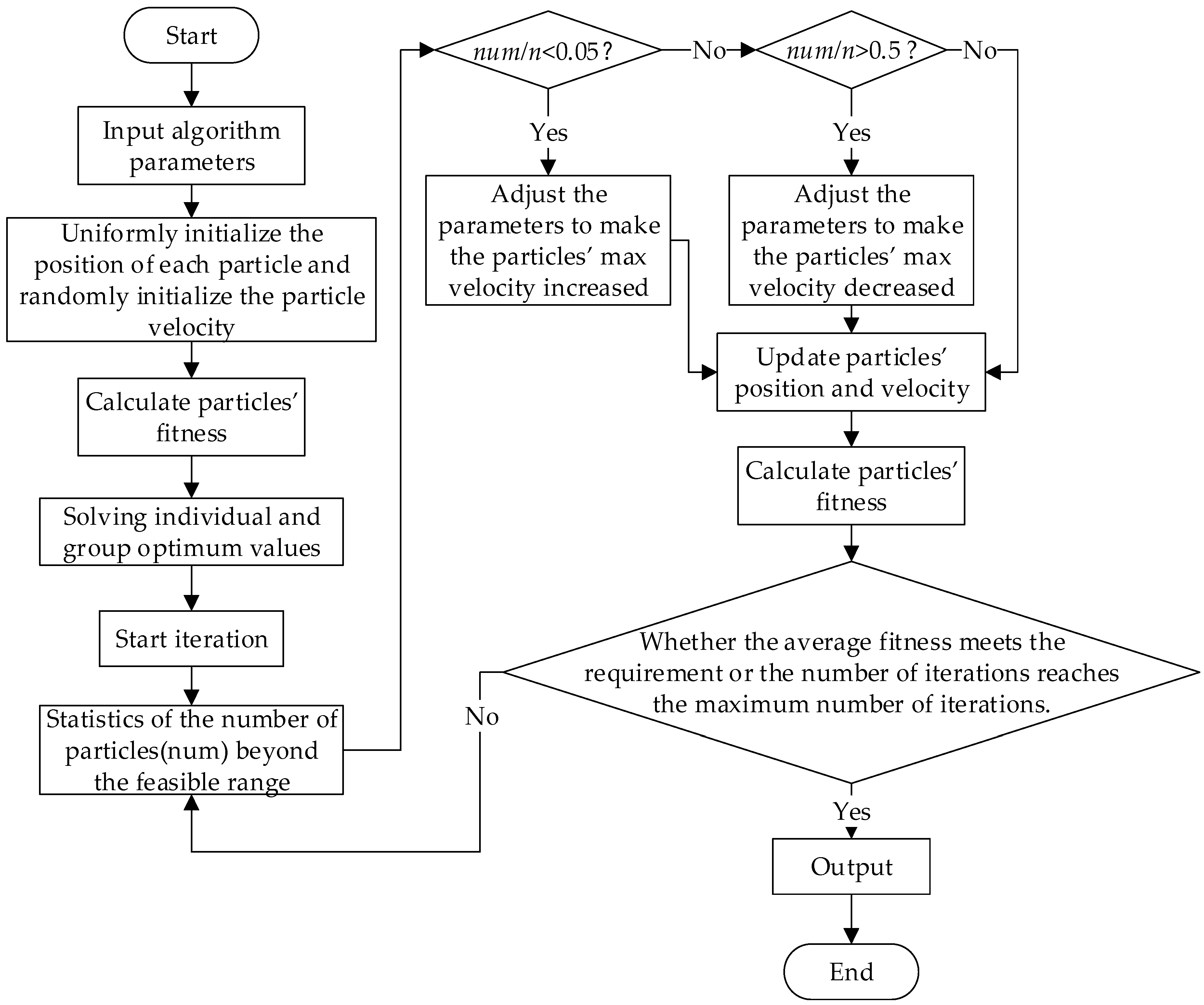
- In a particle swarm optimizer, it is necessary to limit the particles’ positions after updating them in case they exceed the feasible region. In the process of searching for the optimal solution, the number of particles that exceed the feasible region before limiting them can reflect the group’s search status to some extent. If the number is too large, it means that the distribution of the particles is too scattered and the search scope is too large. Then it is necessary to reduce the velocities of the particles by speeding up the attenuation rate of the inertia weight and reducing the maximum velocity allowed. If the number is too small, it means that the particles maybe are gathering too much to do a full search. Then it is necessary to increase the velocities of the particles by slowing down the attenuation rate of the inertia weight and increasing the maximum velocity allowed.
- Give values of all parameters needed in the algorithm, including the number of uniformly division for each dimension m, range of search area ps, range of velocity vs, fitness function adaptfunc, the maximum number of iterations N, and so on.
- Uniformly initialize the population’s positions Xi (i = 1, 2, …, n).
- Randomly initialize population velocity within the range of velocity range.
- Calculating particle fitness using initialized population position.
- Initialize each particle’s best previous position Pi (i = 1, 2, …, n) and the best previous position of all particles Pg by using particle fitness calculated in d-th step.
- Update each particle’s velocity and position according to Equations (1) and (2).
- If the current iteration number does not reach 2/3 of N, then go to step h, otherwise go to step g.
- Count the number of particles, num, that exceed the feasible region after updating. If num/n is greater than 0.5, reduce the velocities of all particles by speeding up the attenuation rate of the inertia weight and reducing the maximum velocity allowed. If num/n is less than 0.05, increase the velocities of the particles by slowing down the attenuation rate of the inertia weight and increasing the maximum velocity allowed. If num/n is somewhere between 0.05 and 0.5, keep the current search status.
- If a dimension of a particle exceeds the upper limit, the dimension information is replaced by the upper limit value, and the lower limit value is replaced by the lower limit value. Then calculate each particle’s fitness.
- Update each particle’s best previous position Pi (i = 1, 2, …, n) and the best previous position of all particles Pg.
- Calculate the average fitness value of the top 50% particles in the population. If the difference between the average fitness values that were respectively calculated during the current iteration and last iteration is less than 0.01 or current iterations t > N, stop the iteration; otherwise go to step f.
3. Support Vector Machine
4. Transverse Flux Induction Heating Optimization Based on VCPSO and SVM
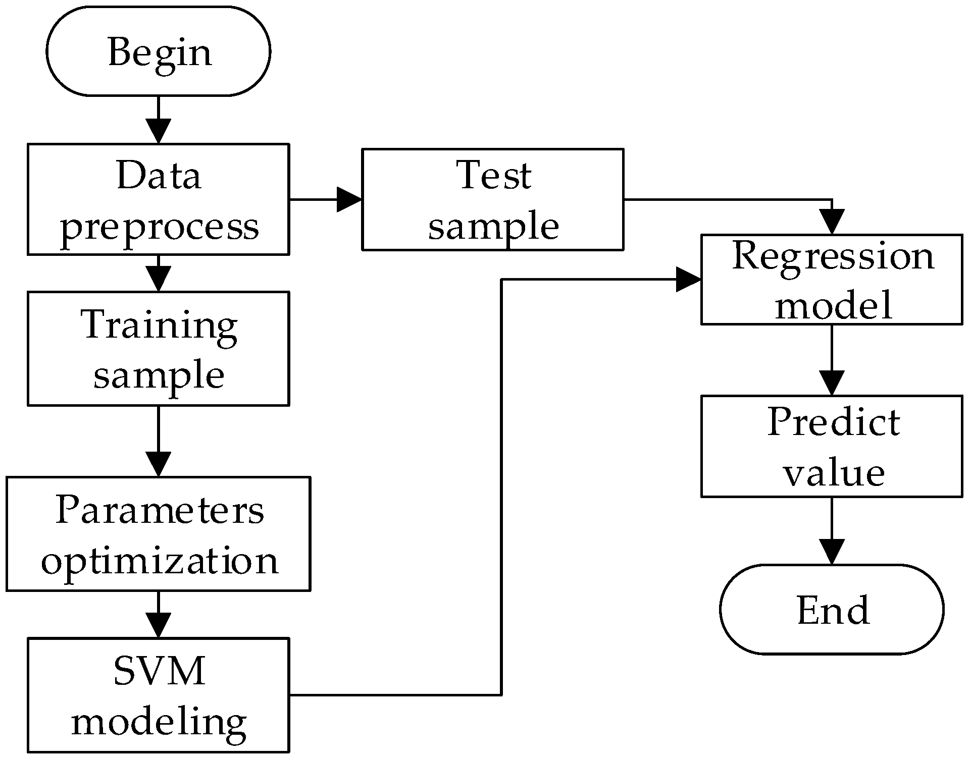
- Original data processing: in order to improve the prediction accuracy, first of all to the original data format, and data will be normalized to [–1, 1]. The normalization has three purpose: (1) to solve the problem of dimension, and if the magnitude difference between different data of the same attribute is too large, the change of large number will cover up the change of decimal number; (2) to improve the convergence speed—the speed of solution can be accelerated after data normalization; (3) to optimize the parameters in the following steps—the larger the input, the better. It is likely that the value of the parameters will exceed the optimum range, and after normalization, the optimum range of the parameters can basically cover its optimum value.
- Training samples and test samples: after data processing, a part of the original data is selected as training samples to establish a regression prediction model, and the rest as test samples to test the accuracy of the obtained prediction model.
- Parameter optimization: the parameters here refer to a series of parameters involved in the modeling process, such as penalty factor, and parameters in the kernel function. When different parameters are selected, the prediction models will be different and the accuracy of the models will be different. Therefore, it is necessary to optimize the parameters to obtain the prediction model with the highest accuracy.
- SVM modeling: the process of solving the corresponding convex quadratic programming problem.
- Regression model: the regression prediction model of transverse flux induction heating problem can be obtained by the above process.
- Finally, the predictive model is used to predict the test sample and get the predictive value. The comparison between predicted and simulated values is shown in Table 3. From the comparison of data in Table 3, it can be seen that the regression prediction model of transverse flux induction heating established by support vector machine has high fitting accuracy, and can be used to replace the finite element numerical calculation to analyze the transverse flux induction heating problem.
5. Conclusions
Author Contributions
Funding
Conflicts of Interest
References
- Pang, L.L.; Wang, Y.H.; Chen, T.G. New development of traveling wave induction heating. IEEE Trans. Appl. Supercond. 2010, 20, 1013–1016. [Google Scholar] [CrossRef]
- Wang, Y.H.; Wang, J.H.; Pang, L.L.; Ho, S.L.; Fu, W.N. An advanced double-layer combined windings transverse flux system for thin strip induction heating. J. Appl. Phys. 2011, 109, 07E511. [Google Scholar] [CrossRef]
- Eberhart, R.C.; Dobbins, R.W.; Simpson, P.K. Computational Intelligence PC Tools; Academic Press: Boston, MA, USA, 1996. [Google Scholar]
- Eberhart, R.C.; Kennedy, J. A new optimizer using particle swarm theory. In Proceedings of the Sixth International Symposium on Micro Machine and Human Science, Nagoya, Japan, 4–6 October 1995; pp. 39–43. [Google Scholar]
- Kennedy, J.; Eberhart, R.C. Particle swarm optimization. In Proceedings of the IEEE International Conference on Neural Networks, Perth, WA, Australia, 27 November–1 December 1995; Volume 4, pp. 1942–1948. [Google Scholar]
- Kennedy, J. The particle swarm: Social adaptation of knowledge. In Proceedings of the IEEE International Conference on Evolutionary Computation, Indianapolis, IN, USA, 13–16 April 1997; pp. 303–308. [Google Scholar]
- Ciuprina, G.; Ioan, D.; Munteanu, I. Use of intelligent-particle swarm optimization in electromagnetics. IEEE Trans. Magn. 2002, 38, 1037–1040. [Google Scholar] [CrossRef]
- Fukuyama, Y.; Takayama, S.; Nakanishi, Y.; Yoshida, H. In A Particle Swarm Optimization for Reactive Power and Voltage Control in Electric Power Systems considering voltage security assessment. In Proceedings of the Conference on Systems, Man, and Cybernetics, Tokyo, Japan, 12–15 October 1999. [Google Scholar]
- Senthil Arumugam, M.; Rao, M.V.C.; Chandramohan, A. A New and Improved Version of Particle Swarm Optimization Algorithm with Global-Local Best Parameters. J. Knowl. Inf. Syst. 2008, 16, 324–350. [Google Scholar] [CrossRef]
- Li, Z.Q.; Zheng, H.; Peng, C.M. Particle Swarm Optimization Algorithm Based on Adaptive Inertia Weight. In Proceedings of the 2010 2nd International Conference on Signal Systems, Dalian, China, 5–7 July 2010; pp. 454–457. [Google Scholar]
- Shi, Y.; Eberhart, R.C. A modified particle swarm optimizer. In Proceedings of the IEEE International Conference on Evolutionary Computation, Anchorage, AK, USA, 4–9 May 1998; pp. 69–73. [Google Scholar]
- Shi, Y.; Eberhart, R.C. Parameter selection in particle swarm optimization. In Proceedings of the International Conference on Evolutionary Programming, Berlin/Heidelberg, Germany, 25–27 March 1998; pp. 591–600. [Google Scholar]
- Shi, Y.; Eberhart, R.C. Empirical study of particle swarm optimization. In Proceedings of the 1999 Congress of Evolutionary Computation, Washington, DC, USA, 6–9 July 1999; pp. 1945–1950. [Google Scholar]
- Coelho, L.d.S. Gaussian quantum-behaved particle swarm optimization approaches for constrained engineering design problems. Expert Syst. Appl. 2010, 37, 1676–1683. [Google Scholar] [CrossRef]
- Fu, K.; Yang, X.G.; Wang, Y.H. The inter generation statistical character self-feedback improved genetic algorithm based on SVM model. In Proceedings of the 1st International Conference on Bioinformatics and Biomedical Engineering, Wuhan, China, 6–8 July 2007; pp. 618–651. [Google Scholar]
- Cristinini, N.; Shawe-taylor, J. An Introduction to Support Vector Machines and other Kernel-Based Learning Methods; Cambridge University Press: Cambridge, UK, 2000. [Google Scholar]
- Hadchum, P.; Wongthanavasu, S. Facial Age Estimation Using a Hybrid of SVM and Fuzzy Logic. In Proceedings of the 2015 12th International Conference on Electrical Engineering/Electronics, Computer, Telecommunications and Information Technology (ECTI-CON), Hua Hin, Thailand, 24–27 June 2015. [Google Scholar]
- Wu, J.; Yang, H. Linear Regression-Based Efficient SVM Learning for Large-Scale Classification. IEEE Trans. Neural Netw. Learn. Syst. 2015, 26, 2357–2369. [Google Scholar] [CrossRef] [PubMed]
- Tyagi, D.; Verma, A.; Sharma, S. An Improved Method for Face Recognition using Local Ternary Pattern with GA and SVM classifier. In Proceedings of the 2016 2nd International Conference on Contemporary Computing and Informatics (IC3I), Noida, India, 14–17 December 2016; pp. 421–426. [Google Scholar]
- Zhu, H.; Liu, X.; Lu, R.; Li, H. Efficient and Privacy-Preserving Online Medical Prediagnosis Framework Using Nonlinear SVM. IEEE J. Biomed. Health Inform. 2017, 21, 838–850. [Google Scholar] [CrossRef] [PubMed]
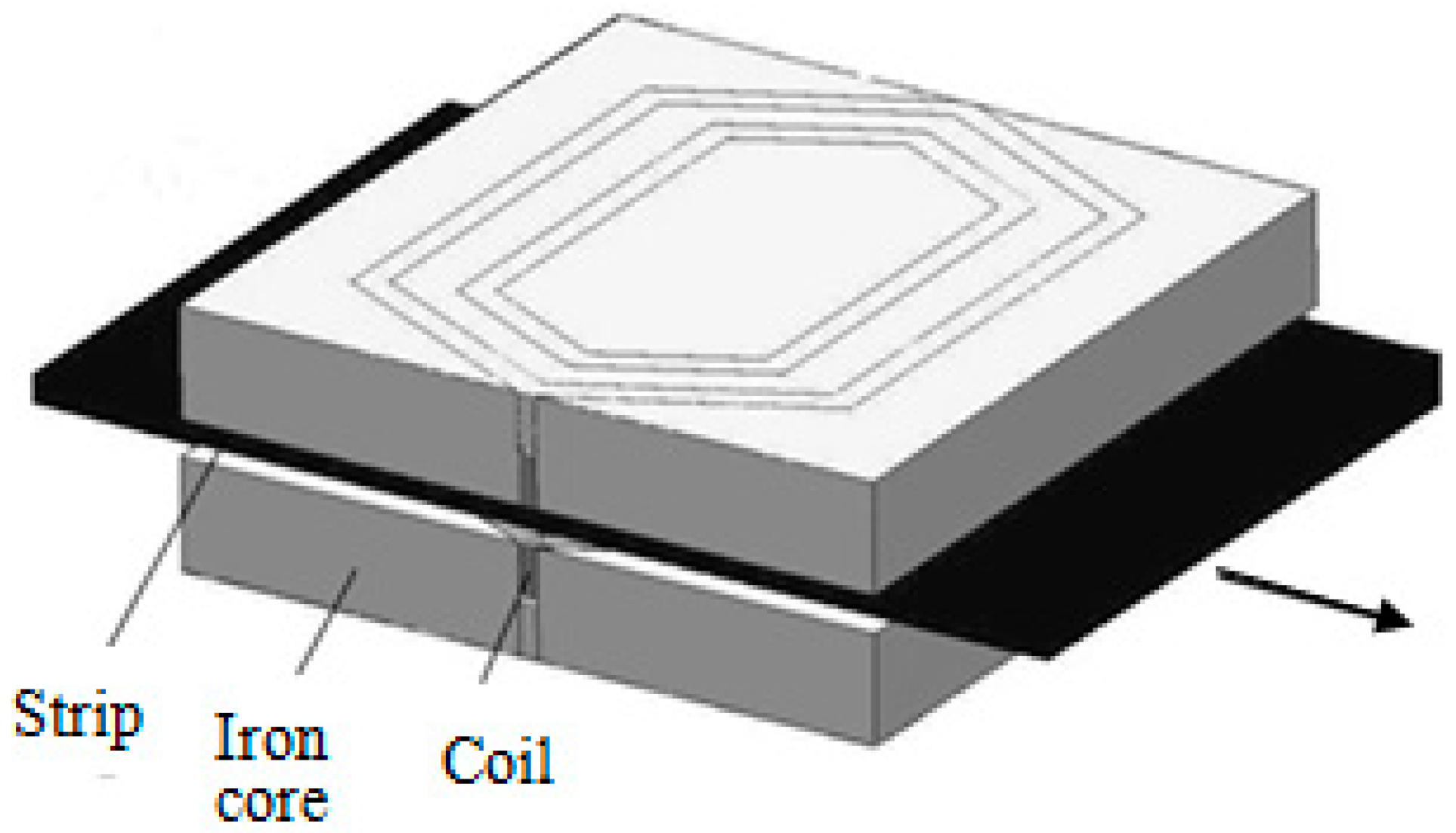
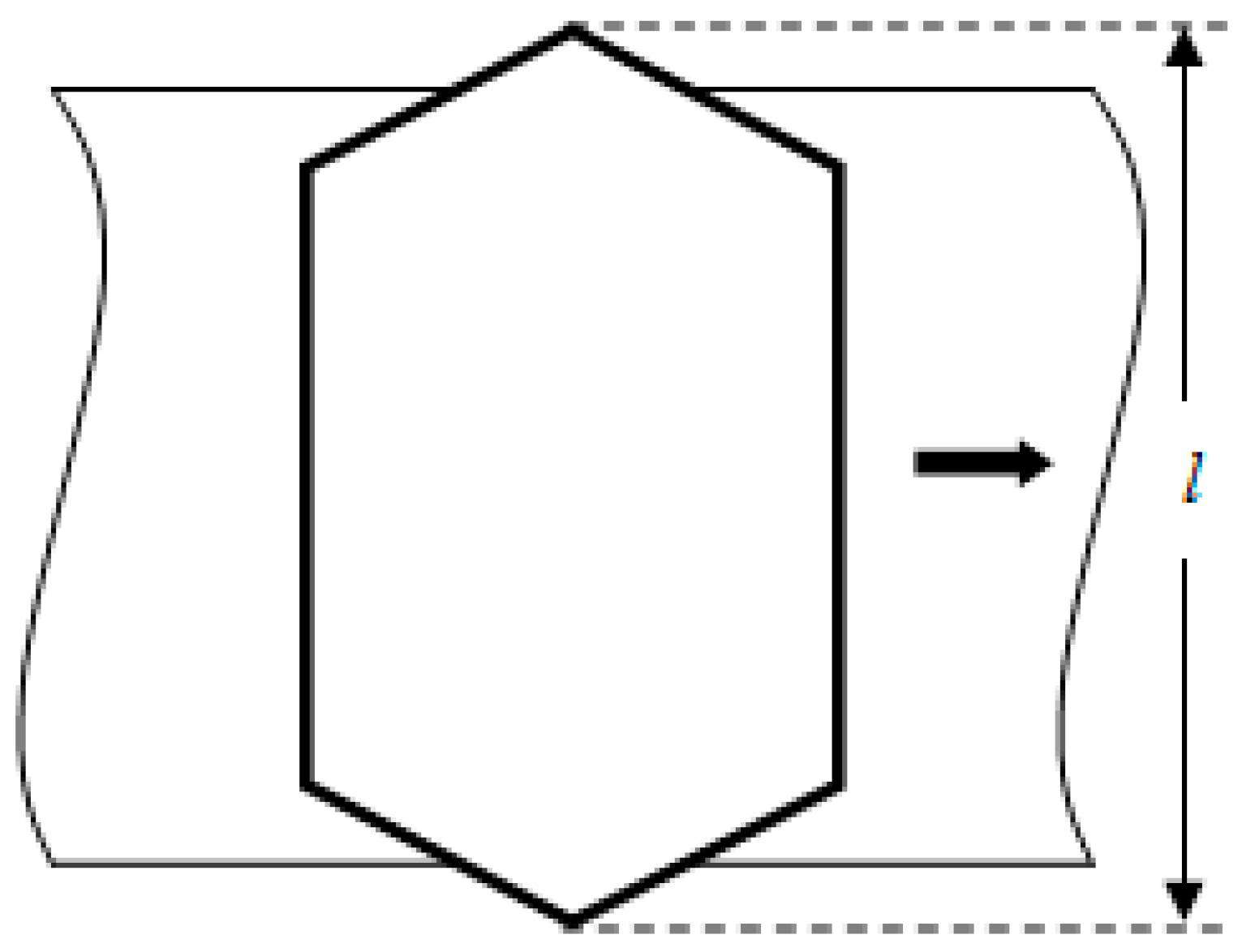
- Sun, Y.; Wang, Y.H.; Yang, X.G.; Pang, L.L. A novel coil shape for transverse flux induction heating. Chin. J. Electr. Eng. 2014, 29, 85–90. [Google Scholar]


| Algorithm | Test Function | Population | Running Time (s) | Average Iterations | Optimal Solution |
|---|---|---|---|---|---|
| f1 | 125 | 0.15 | 75 | 3.0014 | |
| f2 | 1024 | 2.01 | 100 | 5.7421 × 10⁻³ | |
| SPSO | f3 | 1024 | 2.02 | 100 | non |
| f4 | 1024 | 2.74 | 100 | 0.4833 | |
| f5 | 100 | 0.02 | 8 | 3.49620 × 10⁻³ | |
| f1 | 125 | 0.49 | 100 | 9.3634 | |
| f2 | 1024 | 1.21 | 98 | 3.9626 × 10⁻²¹ | |
| GQPSO | f3 | 1024 | 1.99 | 98 | 19.151 × 10⁻²⁴ |
| f4 | 1024 | 2.43 | 100 | 0.4608 × 10⁻⁶ | |
| f5 | 100 | 0.05 | 100 | 0.07 | |
| f1 | 125 | 0.10 | 72 | 3.0006 | |
| f2 | 1024 | 1.07 | 53 | 0 | |
| VCPSO | f3 | 1024 | 1.68 | 89 | 0.6502 × 10⁻³ |
| f4 | 1024 | 1.79 | 60 | 0 | |
| f5 | 100 | 0.01 | 6 | 0 |
| Input Current (A) | Input Frequency (Hz) | Coil Length (mm) | Average Relative Error of Temperature (%) |
|---|---|---|---|
| 400 | 550 | 380 | 0.74 |
| 700 | 550 | 380 | 1.18 |
| 1000 | 550 | 380 | 1.45 |
| 1300 | 550 | 380 | 1.68 |
| 400 | 850 | 380 | 0.71 |
| … | … | … | … |
| 1300 | 1150 | 410 | 8.53 |
| 400 | 1450 | 410 | 7.25 |
| 700 | 1450 | 410 | 8.39 |
| 1000 | 1450 | 410 | 8.54 |
| Input Current (A) | Input Frequency (Hz) | Coil Length (mm) | Average Relative Error of Temperature (%) Finite Element Calculate Value | Average Relative Error of Temperature (%) SVM Predict Value |
|---|---|---|---|---|
| 700 | 1450 | 380 | 2.41 | 2.47 |
| 400 | 550 | 390 | 0.86 | 1.00 |
| 700 | 550 | 400 | 3.91 | 3.56 |
| 1300 | 850 | 410 | 7.34 | 7.27 |
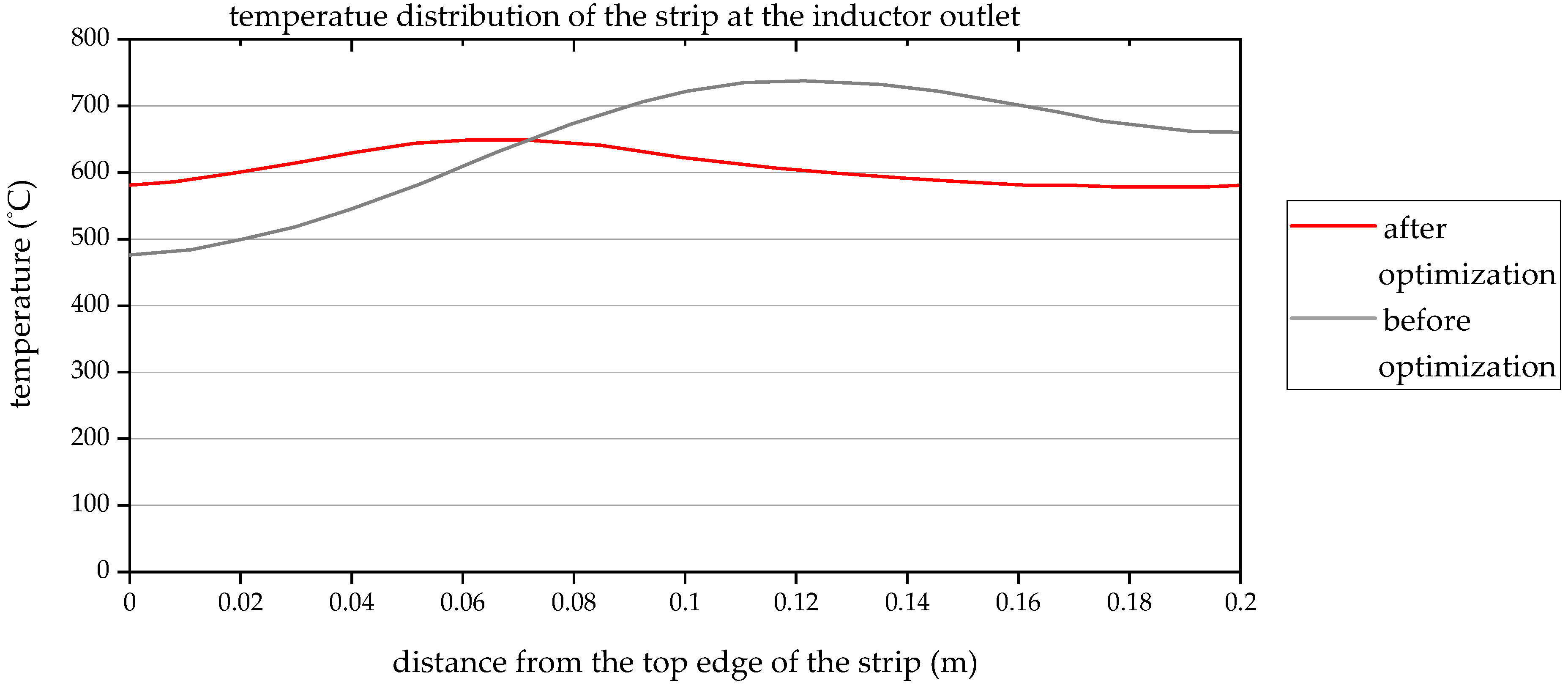
| Optimization Stage | Input Current (A) | Input Frequency (Hz) | Coil Length (mm) |
|---|---|---|---|
| Before optimization | 1000 | 500 | 400 |
| After optimization | 1197 | 1333 | 389 |
© 2019 by the authors. Licensee MDPI, Basel, Switzerland. This article is an open access article distributed under the terms and conditions of the Creative Commons Attribution (CC BY) license (http://creativecommons.org/licenses/by/4.0/).
Share and Cite
Wang, Y.; Li, B.; Yin, L.; Wu, J.; Wu, S.; Liu, C. Velocity-Controlled Particle Swarm Optimization (PSO) and Its Application to the Optimization of Transverse Flux Induction Heating Apparatus. Energies 2019, 12, 487. https://doi.org/10.3390/en12030487
Wang Y, Li B, Yin L, Wu J, Wu S, Liu C. Velocity-Controlled Particle Swarm Optimization (PSO) and Its Application to the Optimization of Transverse Flux Induction Heating Apparatus. Energies. 2019; 12(3):487. https://doi.org/10.3390/en12030487
Chicago/Turabian StyleWang, Youhua, Bin Li, Liuxia Yin, Jiancheng Wu, Shipu Wu, and Chengcheng Liu. 2019. "Velocity-Controlled Particle Swarm Optimization (PSO) and Its Application to the Optimization of Transverse Flux Induction Heating Apparatus" Energies 12, no. 3: 487. https://doi.org/10.3390/en12030487
APA StyleWang, Y., Li, B., Yin, L., Wu, J., Wu, S., & Liu, C. (2019). Velocity-Controlled Particle Swarm Optimization (PSO) and Its Application to the Optimization of Transverse Flux Induction Heating Apparatus. Energies, 12(3), 487. https://doi.org/10.3390/en12030487