Uncertainty Analysis of Factors Influencing Stimulated Fracture Volume in Layered Formation


State Key Laboratory of Oil and Gas Reservoir Geology and Development Engineering, Southwest Petroleum University, Chengdu 610500, China
*
Author to whom correspondence should be addressed.
Energies 2019, 12(23), 4444; https://doi.org/10.3390/en12234444
Submission received: 8 October 2019
/
Revised: 12 November 2019
/
Accepted: 18 November 2019
/
Published: 22 November 2019
(This article belongs to the Section L: Energy Sources)
Abstract
:Hydraulic fracture dimension is one of the key parameters affecting stimulated porous media. In actual fracturing, plentiful uncertain parameters increase the difficulty of fracture dimension prediction, resulting in the difficulty in the monitoring of reservoir productivity. In this paper, we established a three-dimensional model to analyze the key factors on the stimulated reservoir volume (SRV), with the response surface method (RSM). Considering the rock properties and fracturing parameters, we established a multivariate quadratic prediction equation. Simulation results show that the interactions of injection rate (Q), Young’s modulus (E) and permeability coefficient (K), and Poisson’s ratio (μ) play a relatively significant role on SRV. The reservoir with a high Young’s modulus typically generates high pressure, leading to longer fractures and larger SRV. SRV reaches the maximum value when E1 and E2 are high. SRV is negatively correlated with K1. Moreover, maintaining a high injection rate in this layered formation with high E1 and E2, relatively low K1, and μ1 at about 0.25 would be beneficial to form a larger SRV. These results offer new perceptions on the optimization of SRV, helping to improve the productivity in hydraulic fracturing.

1. Introduction
Simulation of hydraulic fracturing contributes to the reservoir characterization and stimulation treatment [1]. On the basis of models, such as Khristianovich–Geertsma–DeKlerk (KGD) model [2], Perkins–Kern–Nordgren (PKN) model [3], penny-shaped fracture model [4], pseudo 3D model [5] and fully 3D hydraulic fracture model [6], the numerical simulation of hydraulic fracturing technology has developed vigorously. Recent researches have expanded the complexity of hydraulic fracturing modeling and improved the mathematical model in simulation in three folds, including: (1) three-dimensional fractures developed near the wellbore [7,8,9]; (2) the interaction between a hydraulic fracture (HF) and natural fracture (NF) [10,11,12]; (3) the stimulated reservoir volume (SRV) of fractured formations [13,14,15,16].
Fracture parameters are closely related to reservoir production in a low permeable formation. Micro-seismic [17] and numerical simulation [18] of hydraulic fracturing indicate that geometric and hydromechanical characteristics of fractures possess the ability to change the well pressure and transient rate performance [19,20,21]. Successful fracturing (large stimulated reservoir volume) leads to greater cumulative production within a short production time [22,23].
Multiple uncertain parameters in actual fracturing increase the difficulty of fracturing design; thus, researches on factors affecting fracturing are studied. Fracturing crack morphology is affected by parameters, such as the geo-mechanical and mechanical properties and the stress distribution of target formation [24,25], and the most crucial parameters affecting fracture design include Young’s modulus, pumping rate, and the in-situ stress contrast [26]. In the case of the same in-situ stress difference, the larger the stress value is, the larger the crack width, and the shorter the crack length will be, thus affecting the degree of stress interference [27]. For a given injection rate, the fracture tip velocity depends on all basic parameters such as leak-off coefficient, modulus, and zone height [28]. Fracture spacing, injection pressure, in-situ stress contrast, and natural fracture dip also affect the geometry of hydraulic fractures [29,30]. Reservoir geo-mechanical parameters and hydromechanical parameters affect the stimulated reservoir volume [31] and oil productivity [32]. And the geological mechanics and hydromechanical parameters of the barrier layer affects SRV, as well, in layered formation. In view of the above studies, the properties of both reservoir and barrier are rarely considered in the analysis of fracturing in layered formation, which can form the interactions and influence the stimulated reservoir volume.
The response surface method (RSM), which can clearly screen out the effects of several process variables and their interactions on response [33], is a good option for fracturing design, and RSM has been applied to the analysis of the multi-factor analysis of hydraulic fracturing under two-dimensional conditions [34]. Wei, et al. [35] found out the controlling factors of fracture height in three dimensions and gave a reasonable optimal design. Yu and Sepehrnoori [36] studied multiple hydraulically fractured horizontal wells in a gas drilling optimization analysis.
The focus of this study is to clarify the key variables and their interactions controlling SRV, and analyze the reasons for the differences in the key factors. We provide a fully three-dimensional benchmark model to study the uncertainty analysis of multiple factors. Actual data from target formation in central-western China were applied to illustrate the effectiveness of the approach. Moreover, by employing RSM to build the response surface with geo-mechanical parameters and hydromechanical parameters and operational parameters, a quadratic response surface model was established.
2. Methodology
A cohesive zone model (CZM) was used to analyze the fluid flow in fractures and fluid–solid coupling in formation, and the response surface method was applied to investigate the key factors of layered formation. A flow chart of the SRV analysis program is presented in Figure 1.
2.1. Theoretical Background
Basic rock deformation-seepage coupling runs through the whole process of hydraulic fracturing. The fluid flow in the rock causes the change of pore pressure, which is acting on the rock matrix deforming the rock; thus, the subsequent structural deformation, in turn, affects the seepage flow. In this paper, it is assumed that the plastic evolution of reservoir rock as porous media follows the Mohr–Coulomb criterion, and the pores of the rock are completely saturated and filled with incompressible fluid, so the mechanical equilibrium equation of the rock deformation is:
Fluid flow continuity equation:
where is the integral space; is the integral space surface; is the effective stress matrix; is the pore pressure; is the matrix vector for the unit; is the strain matrix; is the region outside the surface force; is the virtual velocity matrix; is the unit volume force without regard to fluid gravity; is the porosity; is the pore fluid density; represents the direction parallel to the normal of the outer surface of the integral; is the velocity of fluid flow between rock pores; is the computing time.
Coupling of fracture propagation and fluid flow is a typical nonlinear behavior; thus, reservoir stimulation is a complex process. The cohesive zone model (CZM), which overcomes the stress singularity before the crack tip, is widely used in the nucleation and growth of hydro-fractures in porous elastic formations [37,38]. The constitutive relation in the bond zone reflects the separation and slip of traction and fault surface, and CZM can be adopted using the finite element method (FEM) to investigate hydraulic fracture propagation [39,40,41], including the fracture tip material softening.
where is the normal stress component at the specified point; is critical tensile stress in the normal direction of the element, which represents the tensile strength of reservoir rock; and are the shear stress at specified point; and are the critical shear stress.
Cohesion is a function of the relative displacement of the upper and lower surface of the crack and is controlled by the interface damage factor. When D is 0, the unit exhibits no damage; when D is 1, the crack opens completely. The cohesive element method adopts the damage factor D to describe the crack extension:
where is the displacement value corresponding to the complete failure of the element; is the maximum displacement of the element; is the displacement value corresponding to the occurrence of damage at the beginning of the element.
As the propagation, the process of hydraulic fracturing is usually accompanied by the shear slip effect, and the crack mode is a composite crack. When the element is completely damaged, it means that the cohesion disappears completely, and at the same time, it marks the generation of a new macroscopic crack surface, and the energy consumed in this damage process is the fracture energy. When describing the propagation behavior of composite fractures, the Benzeggagh and Kenane [42] is applied to give the criteria of the critical energy release rate of fracture propagation:
where the B–K criterion assumes that the first and second tangential equals the fracture energy release rate, namely ; is the critical strain energy release rate of normal fracture; is the constants relating to the properties of the material itself; is critical fracture energy release rate for composite fractures.
Fracturing is hydraulically driven, in which the high-pressure fluid in the wellbore is injected into the fracture. The fracturing fluid pressure acting on the fracture surface is the driving force of the fracture expansion. The flow within the cohesive pore pressure element includes a tangential flow along the fracture surface and normal flow along the vertical fracture surface (shown in Figure 2). The mathematic fracture tip corresponds to the point that is about to separate; the cohesive fracture tip is the damage initiation point where the separation reaches the critical value () or the traction reaches the cohesive strength; the material fracture tip refers to the complete failure point where the separation reaches the critical value (), and the traction acting across the unbroken cohesive zone vanishes [43].
The fracturing fluid is regarded as a Newtonian fluid, and the tangential flow on the fracture surface can be written as:
where is the injection rate; is the flow coefficient; ∇ is the fluid pressure gradient along the cohesive zone.
According to the Reynolds number equation, the flow coefficient can be expressed as:
where is the fracture width, the fluid viscosity coefficient.
The filtration coefficient is set to form a permeable layer on the fracture surface, and the normal percolation of the fracturing fluid on the fracture surface can be expressed as:
where is the interfacial fluid pressure of cohesive fracture element; and are, respectively, the seepage flow rate of the fluid on the upper and lower surfaces of the crack; and are, respectively, the fluid loss coefficients on the upper and lower surfaces of the crack; and are, respectively, the fluid pore pressure above and below the fracture surface.
The cohesive fracture zone is filled with fluid, and the fracture of the rock does not produce a traction effect, but the fluid pressure acts on the open fracture surface.
is the injection rate. Substituting Equations (7)–(10) into Equation (11) results in the Reynold’s lubrication equation:
Equation (12) is used to describe the fluid flow in the fracture plane. It can be seen from the equation that there is a pressure-pull-separation relationship between the cohesive fracture zone and the compressed fracture.
2.2. Model Setup
The target formation, in central-western China, is composed of shale, mudstone, and sandstone formed by sedimentation. The upper lithology is mainly mudstone with the inclusion of siltstone, and the lithology of the middle lower part is mainly mudstone, sandstone, and shale. Based on logging data and mechanical rock tests, to study the hydraulic response of SRV to vertical fracture propagation and clarify its key influencing factors, a fully three-dimensional model was established (Figure 3). The overburden of the model was composed of mudstone with a depth range of 1000 to 1020.06 m, while the reservoir was composed of sandstone with a depth range of 1020.06 to 1029.94 m, and the vertical well fracturing was performed in a reservoir. An interval with a depth of 1029.94 to 1050 m was mudstone.
The hydraulic fracturing numerical model follows the following assumptions:
- (1)
- The formation is isotropic pore material.
- (2)
- Initial stress gradient is evenly distributed in each layer.
- (3)
- Interface slippage between reservoir and barrier is not considered.
- (4)
- Fluid in the pores is incompressible.
The unopened vertical fracture surface is described by a nested zero-thickness cohesive zone with the same stiffness as the surrounding rocks, and no initial separation occurred. A total of 19,500 pore pressure structural elements and 23,409 nodes were the basis of the whole numerical model analysis, and the mesh was encrypted around the perforation. The geo-stress field acted on the whole formation model, fixing the lower boundary and constraining the normal displacement of the remaining boundary. The pore pressure boundary condition was set to a certain value of 20 MPa. The minimum horizontal principal stress and the maximum horizontal principal stress were 8 and 12 MPa, respectively. The vertical stress was equal to 10 MPa. The fracturing fluid viscosity was 0.001 Pa∙s. Considering the cohesion and internal friction angle of the mudstone layer and sandstone layer, we adopted Mohr–Coulomb failure criterion to analyze the plastic failure of the rock and calculate the percolation-stress failure process of the rock. The basic parameters used for the numerical simulation are shown in Table 1.
The whole hydraulic fracturing analysis consists of four steps. Firstly, in order to eliminate the displacement caused by gravity and initial conditions, the boundary and initial stress conditions are applied to achieve the geo-stress balance. The results are used in the next step of the hydraulic fracturing calculation. Then, fluid is injected into the central perforation in the reservoir of the model for 100 s: the injection rate increases linearly to 1 × 10⁻² m3/s within 30 s. In the next step, the injection is stopped, and the hydraulic fracture keeps open to simulate proppant behavior, with this stage lasting for 10 s. The final stage totals 1200 s and aims to simulate the fluid back through the fracture, and a production pressure difference of 20 kPa is applied to the perforation node. After stopping the injection, the accumulative high pore pressure in the fracture bleed off into the formation.
2.3. Experimental Design
SRV increases with the optimal combination of various parameters. To study the influence rules of several factors on SRV, the response surface method (RSM) and Box–Behnken Design (BBD) were used to establish multiple quadratic regression models with SRV as a response value.
2.3.1. Response Surface Method
Response surface analysis is a mathematical method based on statistics, which is commonly used in modeling and the analysis of engineering problems [44,45]. Based on the acquired response surface, RSM can quantify the significance of each index and its interaction [46]. In addition, each index and its interaction relationship can be directly displayed by a 3D response surface diagram [33].
SRV was taken as an optimization objective to search for corresponding parameter conditions, and the reasonable experimental design method was adopted to obtain certain data through experiments. The multivariate quadratic regression equation was adopted to fit the functional relationship between factors and response values:
where is the predicted response value; is the independent variable; , , , and are the parameters to be determined in the second-order polynomial mathematical model; is the random error.
In order to discuss whether the model based on RSM approximates the real function, an F statistic was constructed to test significance as follows:
where is the regression sum of squares; is the residual sum of squares; , , are the test value, predicted value, and test mean of the response at point i, respectively; n is the sample size; is the number of independent variables.
2.3.2. Box–Behnken Design
The Box–Behnken experimental design is a cyclic second-order, three-level high (high, medium, and low levels), partial factor experimental design method. This cubic design method is characterized by selecting the midpoints on each side of the multidimensional cube and the midpoints of the cube as design experiments to avoid data loss [47]. As shown in Figure 4, it can be seen that the Box–Behnken design is more efficient than the full three-level factorial design. The total number of tests (N) is defined as: , where is the number of parameters, and is the number of center points. This method can not only overcome the limitations of orthogonal experiments but also reduce the number of experiments and save computing time. Parameters of the model are divided into high, medium, and low levels (140%, 100%, and 60%), and the statistical experimental design is shown in Table 2. These parameters include the injection rate (Q), Young’s modulus (E1, E2), Poisson’s ratio (μ1, μ2), the friction angle (φ1, φ2), the cohesion (C1, C2), the permeability coefficient (K1, K2), the void ratio (ν1, ν2), the dilatancy angle (ψ1, ψ2), and the viscosity (vis1, vis2), and the corresponding meanings of each parameter are shown in Table 2.
3. Results
At the beginning of fracturing in the benchmark model, the injection rate of the fracturing fluid at the perforation rapidly reaches a high level; thus, rock element damage occurs after the pore water pressure rises to the fracture pressure of 39.8 MPa (Figure 5). Pressure waves travel through the reservoir, causing pressure and rate responses [48], which affect the surrounding rock stress and pore pressure in the coupling equation. As the fracture extends upwards and forwards, the fracture height reaches stability outside the reservoir after the fracture crosses the interface of the thin reservoir, and the range of pore water pressure increases.
When t = 16.8 s, the fracture height reaches stability outside the reservoir after the fracture crosses the interface of the thin reservoir (Figure 6). Injection pressure at the fracturing point decreases sharply with the passing of time, and fluctuations appear in the injection pressure curve, but injection pressure gradually stabilizes at about 33.5 MPa. At this time, under the condition of a constant pump injection rate, the fracture begins to expand steadily in the formation, which can be considered as the stable expansion stage of hydraulic fractures [49]. At the end of the fracturing, the resulting fracture size is 32.6 m in length, 13.6 m in height, and 5.8 mm in width.
3.1. Hurricane Analysis of Multiple Factors
Before the response surface analysis, independent factor analyses were carried out for multiple parameters of reservoir and barrier. Geo-mechanical parameters (E, μ, C, φ, ψ), hydromechanical parameters (K, v and vis), and operational parameters (Q) were taken into account to study the influence of each factor. Thirty-four simulation results of SRV indicated that SRV formed by changing diverse variables is dissimilar, as shown in Figure 7. From the hurricane analysis result, the key influencing factors are Q, E2, E1, K1, μ2, μ1, and K2. The BBD experiment was designed for these seven key parameters.
3.2. Response Surface Analysis of Variables to SRV
The interaction between the factors shall not be underestimated [50]. Due to the limitation of the single factor experiments, the continuous point cannot be analyzed, and the interaction among various factors is not considered. Thus, we used the response surface method to comprehensively analyze the results.
SRV is regarded as the function of several influencing factors. The numbers of the simulation experiments were designed to obtain response values, which were established for the mathematical model of the response to each factor level (60%, 100%, 140%). From the above-mentioned hurricane analysis results, seven significant factors (Q, E2, E1, K1, μ2, μ1, K2) were considered in the Box–Behnken experiment design. Sixty-two groups of experiments with different combinations of variables are shown in Table 3, along with corresponding SRV simulation results.
According to the results, the multiple regression equation, including various influencing factors and the interaction of different factors, is established and shown in Equation (17). This equation is based on the actual values of the seven parameters, but in the response surface calculation, the equation is expressed as a combination of coded factors with different coefficients. The high levels of the factors are coded as +1, and the low levels are coded as −1. Parameter coefficients and their standard errors are shown in Figure 8. Comparing parameter coefficients is a supplementary means to identify the relative impact of the seven parameters. In order to discuss the significance of all the model terms, the F-value and p-value were introduced to statistical analysis, as shown in Figure 9. A p-value less than 0.05 implies that the model terms are significant. The statistical results of the F-value and p-value indicate that A, B, C, AB, AC, C2 are the most significant model terms.
Figure 10 shows the comparison between the simulation results of SRV and the prediction value of the response surface. Predicted and actual results are almost distributed in a straight line, and the calibration determination coefficient R2 of the regression equation is 0.973, indicating that the variability of data greater than 95% can be explained by this regression model, with high reliability.
4. Discussion
The established response surface equation consists of seven variables, which are geo-mechanical parameters (E and μ), a geo-physical parameter (K), and an operational parameter (Q). During hydraulic fracturing, the damage and failure mechanisms of the rock are controlled by multiple co-effective properties [51]. Fracture height, width, and injection pressure are sensitive to the variation of material parameters of the reservoir and the barrier (E, μ, and K) [52,53,54]. The effect of variables and their interaction on SRV are emphatically discussed in this section.
4.1. Effect of the Injection Rate
Variations of fracture height, width, and SRV with Q are studied, as shown in Figure 11. When the pump rate increases, the net pressure in hydraulic fractures will increase, resulting in more evident perturbation of formation stress and more fracturing fluid leak-off [55,56,57], and the stimulated reservoir volume will increase. Our statistical results highlight that the injection rate is the most significant factor towards SRV, which is consistent with other researches [34,58,59]. A high pumping rate provides enough energy to overcome resistance, resulting in a larger fracture height and width [11]. Thus, when the pumping rate is low, the hydraulic fracture is incapable of expanding with a wide range. As the injection rate increased to 0.012 m3/s, the created fracture height reaches the maximum level (Figure 11a). However, due to the fracture length at this time being less than the length of the condition of the injection rate of 0.014 m3/s, the value of SRV is not at its maximum. Moreover, a fracture occurs when the local pore pressure at the perforation point reaches the breakdown pressure. When the injection rate is high, the volume of fluid pumped into the fracture per unit time increases, and the pore pressure and skeleton stress at the tip and sides of the hydraulic fracture becomes larger, which causes the breakdown pressure to become higher (Figure 11b).
4.2. Effect of the Young’s Modulus
Sensitivity analyses for the fracture profile and SRV of Young’s modulus are shown in Figure 12 and Figure 13. The interface between strata can produce a barrier effect on the fracture height [60]. When Young’s modulus of the reservoir (E1) is high, the layered formation model tends to be hard, which limits the width and height of the fracture (Figure 12a). The main reason for this control is the coupling effect of the change in crack width and net fracture pressure [61]. Under the condition of a constant injection rate, the net pressure at the crack tip is determined by the fracture width. When Young’s modulus is low, the fracture width in the reservoir and the fluid flow resistance is small. Thus, the corresponding net treatment pressure is low, the fracture length is short, and the resulting fracture volume is small (Figure 12b). The formations with high Young’s modulus typically generate high pressure, leading to longer fractures.
Fracture profiles with the change in Young’s modulus of the barrier (E2) are shown in Figure 12c. The effective Young’s modulus decreased after the fracture penetrated the material interface [62], and the net fracture pressure positively correlated with the effective Young’s modulus.
The stress intensity factor is related to the net crack pressure:
where is the net fracture pressure, and is the fracture height.
The decrease of results in a lower stress intensity factor. Thus, after the penetration of the fracture through the barrier, decreases with the decrease in effective Young’s modulus. The fracture length in the reservoir increases with the increase in E2, resulting in larger SRV (Figure 12d), but there is no significant change in breakdown pressure.
In general, the fracture width depends on the joint action of Young’s modulus of reservoir and barrier. Our statistical results show that SRV reaches the maximum value when E1 and E2 are high, which indicates that E1 and E2 are positively correlated with SRV (Figure 13).
4.3. Effect of the Poisson’s Ratio
T-stress at the crack tip and Poisson’s ratio affect the three typical types of fractures in fracture mechanics. Fracture parameters, including stress intensity factor and t-stress, are related to Poisson’s ratio.
T-stress can be defined as:
where is the thickness strain component, I is the interaction integral, and f is the point force [63]. is positively correlated with μ.
The fracture morphology and SRV with the change of μ are shown in Figure 14. When the reservoir Poisson’s ratio (μ1) is low, the fracture is wide (Figure 14a), but the SRV reaches the maximum and is negatively correlated with μ1 (Figure 14b). That is because the material stress intensity factor and T-stress decrease with the decrease of the Poisson’s ratio. Once the tip of the fracture crosses the interface, the high barrier Poisson’s ratio (μ2) has a relatively weak effect on inhibiting the fracture growth (Figure 14c), and consequently, increasing the fracture extension range (Figure 14d). Lower breakdown pressure leads to easier initiation of hydraulic fractures. Combined with Figure 14 and Figure 15, when μ1 is 0.25, the breakdown pressure is relatively low, and as a result, SRV is optimized.
4.4. Effect of the Permeability Coefficient
Matrix porosity and permeability are sensitive to effective stress and pore pressure [64]. Figure 16 shows the fracture morphology and changes of SRV with the permeability coefficient. When the reservoir permeability coefficient (K1) is low, the formed fracture is relatively narrow (Figure 16a). This is because the lower the permeability, the greater the fluid flow resistance in the formation, and the lower openness the fracture will develop. However, SRV is negatively correlated with K1 (Figure 16b). The mechanism is that the lower the permeability, the easier it is for fluid to flow in the fracture, and the more fluid remains in the fracture rather than being lost in the formation. Thus, a larger fracture volume can be formed.
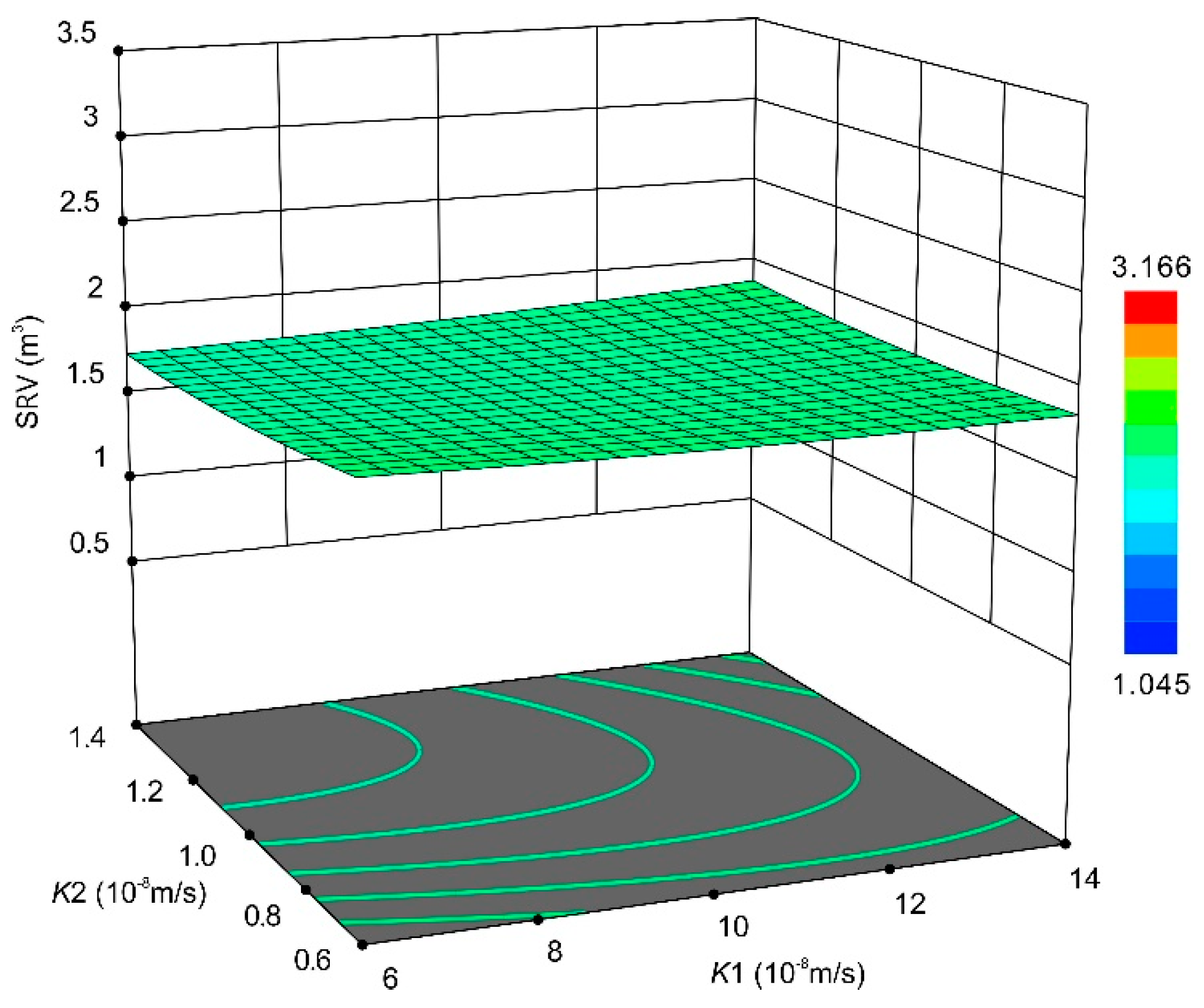
The barrier permeability coefficient (K2) is an order of magnitude smaller than K1; thus, the fluid is mainly in the fracture rather than in the barrier. Increasing K2 can reduce fluid resistance in the barrier, leading to an appropriate increase in the fracture length and width (Figure 16c). So, a larger SRV is formed with the increase of K2 (Figure 16d). The simulation result, as shown in Figure 17, indicates that when K2 is greater than 1.1 10−8 m/s, SRV increases with the increase of K1. That is because K2 and K1 almost remain at the same order of magnitude, the interlayer barrier effect in layered formation is no longer significant, and the fracture length in the reservoir increases.
5. Conclusions
In this paper, the evolution of the morphological characteristics of hydraulic fractures during the whole process of hydraulic fracturing were studied. Using the cohesive zone method, we investigated the effect of each characteristic parameter on SRV and established a quadratic model. The main conclusions are as follows:
- (1)
- To screen the significant influencing factors and determine the optimal level combination, the quadratic response surface model was established. The statistical analysis of the F value and p-value of regression equations implies that the model has a high degree of fitting, which is beneficial for analyzing and predicting the hydraulic behavior of fracturing in a layered formation.
- (2)
- The injection rate and Young’s modulus are the most significant factors to SRV among all the independent variables. A high pumping rate provides enough energy to form a hydraulic fracture with a wide range. The reservoir with high Young’s modulus typically generates high pressure, leading to longer fractures and larger SRV. SRV reaches the maximum value when E1 and E2 are high, which indicates that E1 and E2 are positively correlated with SRV.
- (3)
- When the reservoir Poisson’s ratio (μ1) is low, the fracture is wide, but the SRV reaches the maximum and is negatively correlated with μ1. Once the tip of the fracture crosses the interface, the high barrier Poisson’s ratio (μ2) has a relatively weak effect on inhibiting the fracture growth, and consequently, increasing the fracture extension range. Moreover, the lower the reservoir permeability coefficient (K1), the more fluid remains in the fracture rather than being lost in the formation; thus, SRV is negatively correlated with K1.
- (4)
- Different interactions affect the SRV to varying degrees. In general, maintaining a high injection rate in this layered formation with high E1 and E2, and relatively low K1 and μ1 at about 0.25, would be beneficial to form a larger SRV.
Author Contributions
Conceptualization, X.L., L.L., J.X. and W.L.; Methodology, X.L. and X.W.; Software, J.Z.; Investigation, J.Z. and X.W.; Data Curation, L.L.; Writing-Original Draft Preparation, J.Z.; Writing-Review & Editing, J.Z., X.W. and W.L.
Funding
This research was funded by the National Natural Science Foundation of China (NSFC) under grant no. 51809220, the Open Research Fund of the State Energy Center for Shale Oil Research and Development under grant no. G5800-17ZS-KFNY007, and the Open Research Fund of the State Key Laboratory of Geomechanics and Geotechnical Engineering under grant no. Z017008.
Conflicts of Interest
The authors declare no conflict of interest.
References
- Lecampion, B.; Bunger, A.; Zhang, X. Numerical methods for hydraulic fracture propagation: A review of recent trends. J. Nat. Gas Sci. Eng. 2018, 49, 66–83. [Google Scholar] [CrossRef]
- Daneshy, A.A. On the design of vertical hydraulic fractures. J. Pet. Technol. 1973, 25, 83–97. [Google Scholar] [CrossRef]
- Nordgren, R. Propagation of a vertical hydraulic fracture. Soc. Pet. Eng. J. 1972, 12, 306–314. [Google Scholar] [CrossRef]
- Abé, H.; Keer, L.M.; Mura, T. Growth rate of a penny-shaped crack in hydraulic fracturing of rocks, 2. J. Geophys. Res. 1976, 81, 6292–6298. [Google Scholar] [CrossRef]
- Settari, A.; Cleary, M.P. Development and testing of a pseudo-three-dimensional model of hydraulic fracture geometry. SPE Prod. Eng. 1986, 1, 449–466. [Google Scholar] [CrossRef]
- Carter, B.; Desroches, J.; Ingraffea, A.; Wawrzynek, P. Simulating fully 3D hydraulic fracturing. Model. Geomech. 2000, 200, 525–557. [Google Scholar]
- Park, S.; Kim, K.-I.; Kwon, S.; Yoo, H.; Xie, L.; Min, K.-B.; Kim, K.Y. Development of a hydraulic stimulation simulator toolbox for enhanced geothermal system design. Renew. Energy 2018, 118, 879–895. [Google Scholar] [CrossRef]
- Clarkson, C.R.; Williams-Kovacs, J.D. A New Method for Modeling Multi-Phase Flowback of Multi-Fractured Horizontal Tight Oil Wells to Determine Hydraulic Fracture Properties. In Proceedings of the SPE Annual Technical Conference and Exhibition, New Orleans, LA, USA, 30 September–2 October 2013. [Google Scholar]
- Dongyan, F.; Jun, Y.; Hai, S.; Hui, Z.; Wei, W. A composite model of hydraulic fractured horizontal well with stimulated reservoir volume in tight oil & gas reservoir. J. Nat. Gas Sci. Eng. 2015, 24, 115–123. [Google Scholar]
- Li, Y.; Deng, J.G.; Liu, W.; Feng, Y. Modeling hydraulic fracture propagation using cohesive zone model equipped with frictional contact capability. Comput. Geotech. 2017, 91, 58–70. [Google Scholar] [CrossRef]
- Guo, J.; Luo, B.; Lu, C.; Lai, J.; Ren, J. Numerical investigation of hydraulic fracture propagation in a layered reservoir using the cohesive zone method. Eng. Fract. Mech. 2017, 186, 195–207. [Google Scholar] [CrossRef]
- Wang, X.; Shi, F.; Liu, C.; Lu, D.; Liu, H.; Wu, H. Extended finite element simulation of fracture network propagation in formation containing frictional and cemented natural fractures. J. Nat. Gas Sci. Eng. 2018, 50, 309–324. [Google Scholar] [CrossRef]
- Ren, J.; Guo, P. Nonlinear flow model of multiple fractured horizontal wells with stimulated reservoir volume including the quadratic gradient term. J. Hydrol. 2017, 554, 155–172. [Google Scholar] [CrossRef]
- Guo, T.; Wang, X.; Li, Z.; Gong, F.; Lin, Q.; Qu, Z.; Lv, W.; Tian, Q.; Xie, Z. Numerical simulation study on fracture propagation of zipper and synchronous fracturing in hydrogen energy development. Int. J. Hydrogen Energy 2019, 44, 5270–5285. [Google Scholar] [CrossRef]
- Li, Q.; Lu, Y.; Ge, Z.; Zhou, Z.; Zheng, J.; Xiao, S. A New Tree-Type Fracturing Method for Stimulating Coal Seam Gas Reservoirs. Energies 2017, 10, 1388. [Google Scholar] [CrossRef]
- Wang, W.; Su, Y.; Yuan, B.; Wang, K.; Cao, X. Numerical Simulation of Fluid Flow through Fractal-Based Discrete Fractured Network. Energies 2018, 11, 286. [Google Scholar] [CrossRef]
- Cipolla, C.L.; Maxwell, S.C.; Mack, M.G. Engineering Guide to the Application of Microseismic Interpretations. In Proceedings of the SPE Hydraulic Fracturing Technology Conference, The Woodlands, TX, USA, 6–8 February 2012; Society of Petroleum Engineers: The Woodlands, TX, USA, 2012. [Google Scholar]
- Patterson, R.; Yu, W.; Wu, K. Integration of microseismic data, completion data, and production data to characterize fracture geometry in the Permian Basin. J. Nat. Gas Sci. Eng. 2018, 56, 62–71. [Google Scholar] [CrossRef]
- Zhao, Y.-L.; Zhang, L.-H.; Luo, J.-X.; Zhang, B.-N. Performance of fractured horizontal well with stimulated reservoir volume in unconventional gas reservoir. J. Hydrol. 2014, 512, 447–456. [Google Scholar] [CrossRef]
- Al-Rbeawi, S. How much stimulated reservoir volume and induced matrix permeability could enhance unconventional reservoir performance. J. Nat. Gas Sci. Eng. 2017, 46, 764–781. [Google Scholar] [CrossRef]
- Li, W.; Schmitt, D.R.; Tibbo, M.; Zou, C. A Program to Calculate the State of Stress in The Vicinity of an Inclined Borehole Through an Anisotropic Rock Formation. Geophysics 2019, 84, 1–88. [Google Scholar] [CrossRef]
- Tian, F.; Du, X.; Wang, X.; Xu, W. Rate decline analysis for finite conductivity vertical fractured gas wells produced under a variable inner boundary condition. J. Pet. Sci. Eng. 2018, 171, 1249–1259. [Google Scholar] [CrossRef]
- Zhang, D.; Dai, Y.; Ma, X.; Zhang, L.; Zhong, B.; Wu, J.; Tao, Z. An Analysis for the Influences of Fracture Network System on Multi-Stage Fractured Horizontal Well Productivity in Shale Gas Reservoirs. Energies 2018, 11, 414. [Google Scholar] [CrossRef]
- Chen, C.; Yang, L.; Jia, R.; Sun, Y.; Guo, W.; Chen, Y.; Li, X. Simulation study on the effect of fracturing technology on the production efficiency of natural gas hydrate. Energies 2017, 10, 1241. [Google Scholar] [CrossRef]
- Dong, T.; Harris, N.B.; Ayranci, K.; Yang, S. The impact of rock composition on geomechanical properties of a shale formation: Middle and Upper Devonian Horn River Group shale, Northeast British Columbia, Canada. AAPG Bull. 2017, 101, 177–204. [Google Scholar] [CrossRef]
- Ripudaman, M.; Mani, S.M.; Shawn, H. Time-dependent fracture-interference effects in pad wells. SPE Prod. Oper. 2014, 29, 274–287. [Google Scholar]
- Wang, X.; Liu, C.; Wang, H.; Liu, H.; Wu, H. Comparison of consecutive and alternate hydraulic fracturing in horizontal wells using XFEM-based cohesive zone method. J. Pet. Sci. Eng. 2016, 143, 14–25. [Google Scholar] [CrossRef]
- Weng, X.; Settari, A.; Keck, R.G. A field demonstration of hydraulic fracturing for solids waste disposal—Injection pressure analysis. Int. J. Rock Mech. Min. Sci. 1997, 34, 331. [Google Scholar] [CrossRef]
- Wu, K.; Olson, J.E. Investigation of the impact of fracture spacing and fluid properties for interfering simultaneously or sequentially generated hydraulic fractures. SPE Prod. Oper. 2013, 28, 427–436. [Google Scholar] [CrossRef]
- Chen, Z.; Jeffrey, R.G.; Zhang, X.; Kear, J. Finite-element simulation of a hydraulic fracture interacting with a natural fracture. SPE J. 2017, 22, 219–234. [Google Scholar] [CrossRef]
- Yong, Y.K.; Maulianda, B.; Wee, S.C.; Mohshim, D.; Elraies, K.A.; Wong, R.C.K.; Gates, I.D.; Eaton, D. Determination of stimulated reservoir volume and anisotropic permeability using analytical modelling of microseismic and hydraulic fracturing parameters. J. Nat. Gas Sci. Eng. 2018, 58, 234–240. [Google Scholar] [CrossRef]
- Ashley, W.J.; Panja, P.; Deo, M. Surrogate models for production performance from heterogeneous shales. J. Pet. Sci. Eng. 2017, 159, 244–256. [Google Scholar] [CrossRef]
- Myers, R.H.; Montgomery, D.C.; Anderson-Cook, C.M. Response Surface Methodology: Process. and Product Optimization Using Designed Experiments; John Wiley & Sons: Hoboken, NJ, USA, 2016. [Google Scholar]
- Wang, Y.; Li, X.; Zhang, B.; Zhao, Z. Optimization of multiple hydraulically fractured factors to maximize the stimulated reservoir volume in silty laminated shale formation, Southeastern Ordos Basin, China. J. Pet. Sci. Eng. 2016, 145, 370–381. [Google Scholar] [CrossRef]
- Wei, X.; Fan, X.; Li, F.; Liu, X.; Liang, L.; Li, Q. Uncertainty analysis of hydraulic fracture height containment in a layered formation. Environ. Earth Sci. 2018, 77, 664. [Google Scholar] [CrossRef]
- Yu, W.; Sepehrnoori, K. Optimization of Multiple Hydraulically Fractured Horizontal Wells in Unconventional Gas Reservoirs. J. Pet. Eng. 2013, 2013, 151898. [Google Scholar]
- Dugdale, D.S. Yielding of steel sheets containing slits. J. Mech. Phys. Solids 1960, 8, 100–104. [Google Scholar] [CrossRef]
- Barenblatt, G.I. The mathematical theory of equilibrium cracks in brittle fracture. Adv. Appl. Mech. 1962, 7, 55–129. [Google Scholar]
- Shen, X.; Cullick, S. Numerical Modeling of Fracture Complexity with Application to Production Stimulation. In Proceedings of the SPE Hydraulic Fracturing Technology Conference, The Woodlands, TX, USA, 6–8 February 2012; Society of Petroleum Engineers: The Woodlands, TX, USA, 2012. [Google Scholar]
- Yao, Y. Linear elastic and cohesive fracture analysis to model hydraulic fracture in brittle and ductile rocks. Rock Mech. Rock Eng. 2012, 45, 375–387. [Google Scholar] [CrossRef]
- Carrier, B.; Granet, S. Numerical modeling of hydraulic fracture problem in permeable medium using cohesive zone model. Eng. Fract. Mech. 2012, 79, 312–328. [Google Scholar] [CrossRef] [Green Version]
- Benzeggagh, M.L.; Kenane, M.J.C.S. Measurement of mixed-mode delamination fracture toughness of unidirectional glass/epoxy composites with mixed-mode bending apparatus. Compos. Sci. Technol. 1996, 56, 439–449. [Google Scholar] [CrossRef]
- Shet, C.; Chandra, N. Analysis of energy balance when using cohesive zone models to simulate fracture processes. J. Eng. Mater. Technol. 2002, 124, 440–450. [Google Scholar] [CrossRef]
- Box, G.E.P.; Hunter, J.S. Multi-Factor Experimental Designs for Exploring Response Surfaces. Ann. Math. Stat. 1957, 28, 195–241. [Google Scholar] [CrossRef]
- Box, G.E.; Wilson, K.B. On the experimental attainment of optimum conditions. J. Royal Stat. Soc. Ser. B 1951, 13, 270–310. [Google Scholar] [CrossRef]
- Steinberg, D.M.; Kenett, R.S. Response Surface Methodology; Wiley: Hoboken, NJ, USA, 2009; pp. 1171–1179. [Google Scholar]
- Box, G.E.; Behnken, D.W. Some new three level designs for the study of quantitative variables. Technometrics 1960, 2, 455–475. [Google Scholar] [CrossRef]
- Yang, C.; Sharma, V.K.; Datta-Gupta, A.; King, M.J. Novel approach for production transient analysis of shale reservoirs using the drainage volume derivative. J. Pet. Sci. Eng. 2017, 159, 8–24. [Google Scholar] [CrossRef]
- Zou, J.; Chen, W.; Yuan, J.; Yang, D.; Yang, J. 3-D numerical simulation of hydraulic fracturing in a CBM reservoir. J. Nat. Gas Sci. Eng. 2017, 37, 386–396. [Google Scholar] [CrossRef]
- Yang, L.; Chen, C.; Jia, R.; Sun, Y.; Guo, W.; Pan, D.; Li, X.; Chen, Y. Influence of Reservoir Stimulation on Marine Gas Hydrate Conversion Efficiency in Different Accumulation Conditions. Energies 2018, 11, 339. [Google Scholar] [CrossRef] [Green Version]
- Conrad, J.J.; Cook, N.G.; Zimmerman, R. Fundamentals of Rock Mechanics; John Wiley & Sons: Hoboken, NJ, USA, 2009. [Google Scholar]
- Haddad, M.; Sepehrnoori, K. Simulation of hydraulic fracturing in quasi-brittle shale formations using characterized cohesive layer: Stimulation controlling factors. J. Unconv. Oil Gas Resour. 2015, 9, 65–83. [Google Scholar] [CrossRef]
- Afsar, F. Fracture Propagation and Reservoir Permeability in Limestone-Marl Alternations of the Jurassic Blue Lias Formation (Bristol Channel Basin, UK). Ph.D. Thesis, Georg-August-Universität Göttingen, Göttingen, Germany, 2015. [Google Scholar]
- Wu, C.-Y.; Chiu, Y.-C.; Huang, Y.-J.; Hsieh, B.-Z. Effects of Geomechanical Mechanisms on Gas Production Behavior: A Simulation Study of a Class-3 Hydrate Deposit of Four-Way-Closure Ridge Offshore Southwestern Taiwan. In Proceedings of the European Geosciences Union General Assembly, Vienna, Austria, 22–28 April 2017; Energy Procedia: Vienna, Austria, 2017; pp. 486–493. [Google Scholar]
- Ren, L.; Lin, R.; Zhao, J.; Rasouli, V.; Zhao, J.; Yang, H. Stimulated reservoir volume estimation for shale gas fracturing: Mechanism and modeling approach. J. Pet. Sci. Eng. 2018, 166, 290–304. [Google Scholar] [CrossRef]
- Liu, C.; Jin, X.; Shi, F.; Lu, D.; Liu, H.; Wu, H. Numerical investigation on the critical factors in successfully creating fracture network in heterogeneous shale reservoirs. J. Nat. Gas Sci. Eng. 2018, 59, 427–439. [Google Scholar] [CrossRef]
- Chen, Z.; Jeffrey, R.G.; Zhang, X. Numerical modeling of three-dimensional T-shaped hydraulic fractures in coal seams using a cohesive zone finite element model. Hydraul. Fract. J. 2015, 2, 20–37. [Google Scholar]
- Nagel, N.; Gil, I.; Sanchez-Nagel, M.; Damjanac, B. Simulating hydraulic fracturing in real fractured rock—Overcoming the limits of pseudo 3D models. In Proceedings of the SPE HFTC, Woodlands, TX, USA, 24–26 January 2011; SPE HFTC: The Woodlands, TX, USA, 2011. [Google Scholar]
- King, G.E. Thirty years of gas shale fracturing: What have we learned? In Proceedings of the SPE Annual Technical Conference and Exhibition, Florence, Italy, 19–22 September 2010; Society of Petroleum Engineers: The Woodlands, TX, USA, 2010. [Google Scholar]
- Xing, P.; Yoshioka, K.; Adachi, J.; El-Fayoumi, A.; Bunger, A.P. Laboratory measurement of tip and global behavior for zero-toughness hydraulic fractures with circular and blade-shaped (PKN) geometry. J. Mech. Phys. Solids 2017, 104, 172–186. [Google Scholar] [CrossRef]
- Gu, H.; Siebrits, E. Effect of Formation Modulus Contrast on Hydraulic Fracture Height Containment. SPE Prod. Oper. 2008, 23, 170–176. [Google Scholar] [CrossRef]
- Yue, K. Height Containment of Hydraulic Fractures in Layered Reservoirs. Ph.D. Thesis, University of Texas at Austin, Austin, TX, USA, 2017. [Google Scholar]
- Aliha, M.R.M.; Saghafi, H. The effects of thickness and Poisson’s ratio on 3D mixed-mode fracture. Eng. Fract. Mech. 2013, 98, 15–28. [Google Scholar] [CrossRef]
- Jia, B.; Tsau, J.-S.; Barati, R. Experimental and numerical investigations of permeability in heterogeneous fractured tight porous media. J. Nat. Gas Sci. Eng. 2018, 58, 216–233. [Google Scholar] [CrossRef]
Figure 1.
Flow chart of stimulated reservoir volume (SRV) analysis program is divided into three modules: (1) establishment of a fully three-dimensional model based on logging data and rock mechanics tests; (2) identification of the main control factors according to the simulation results; (3) conduction of Box–Behnken design on SRV, then analyze the effects of several factors and their interactions with the response value.

Figure 2.
Schematic of fluid flow at the fracture tip. The cohesive zone in a hydraulic fracture is classified into a broken cohesive zone and unbroken cohesive zone. The flow of the fluid within the cohesive element includes tangential flow and normal flow.
Figure 2.
Schematic of fluid flow at the fracture tip. The cohesive zone in a hydraulic fracture is classified into a broken cohesive zone and unbroken cohesive zone. The flow of the fluid within the cohesive element includes tangential flow and normal flow.
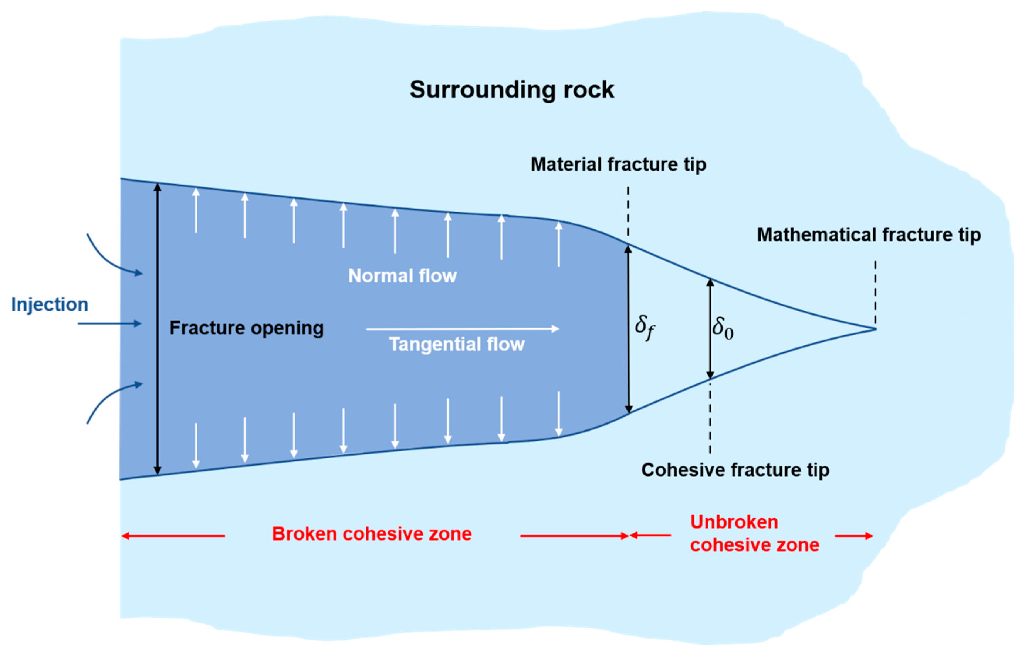
Figure 3.
Hydraulic fracturing calculation model. (a) A 3D geological structure and (b) representation of the calculation model with applied boundary conditions. Fracturing is carried out in the reservoir, and with the increase of fracturing time, hydraulic fracture gradually extends to the barrier.

Figure 4.
Contrast between the full three-level factorial design and the Box–Behnken design. Blue points and lines, located on a hypersphere equidistant from the central point, represent different experiments of Box–Behnken design for three variables. Together with black points and lines, the full three-level factorial design is described.
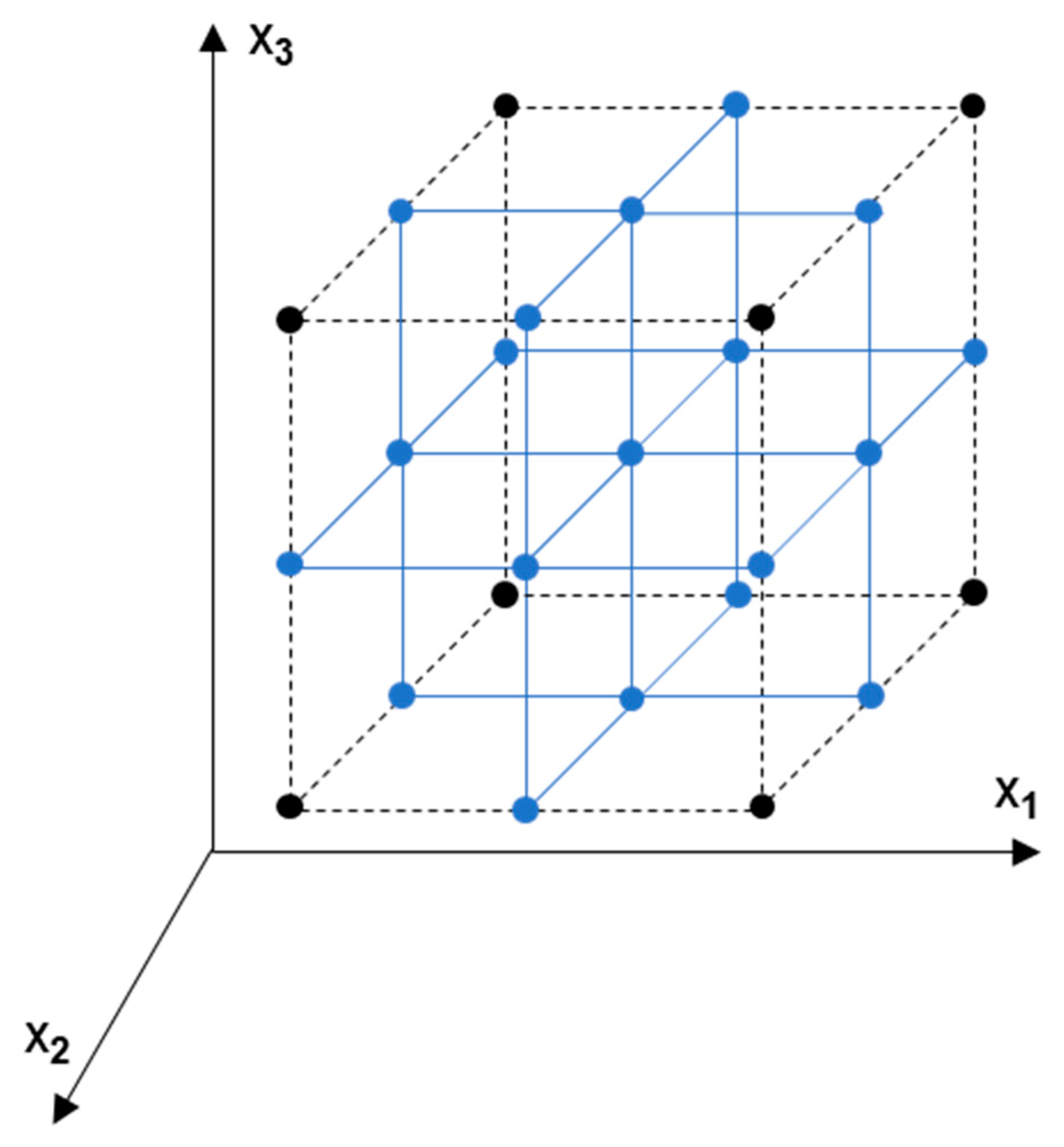
Figure 5.
The change in pore pressure during the fluid injection process in the benchmark model. ① Fluid is injected into the central perforation in the reservoir of the model for 100 s, and pore pressure rapidly rises to the breakdown pressure and gradually stabilizes at a stable level. ② Injection is stopped, and the hydraulic fracture keeps open, proppant acts at this stage, and then dissipated pore pressure activates the production pressure difference to make the fluid move back through the fracture. The research focus is on the fluid injection stage when SRV is formed.
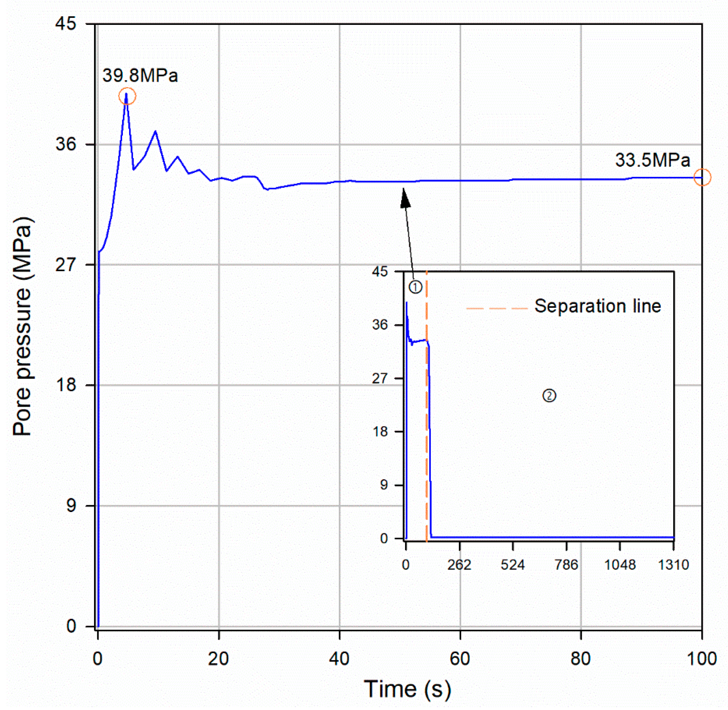
Figure 6.
Fracture width at different times. (a) t = 5 s, (b) t = 16.8 s and (c) t = 100 s.

Figure 7.
Hurricane analysis results for SRV. Indicators of the model are divided into high, medium, and low levels (140%, 100%, and 60%). The dotted gray line in this figure refers to the result of the benchmark model.
Figure 7.
Hurricane analysis results for SRV. Indicators of the model are divided into high, medium, and low levels (140%, 100%, and 60%). The dotted gray line in this figure refers to the result of the benchmark model.
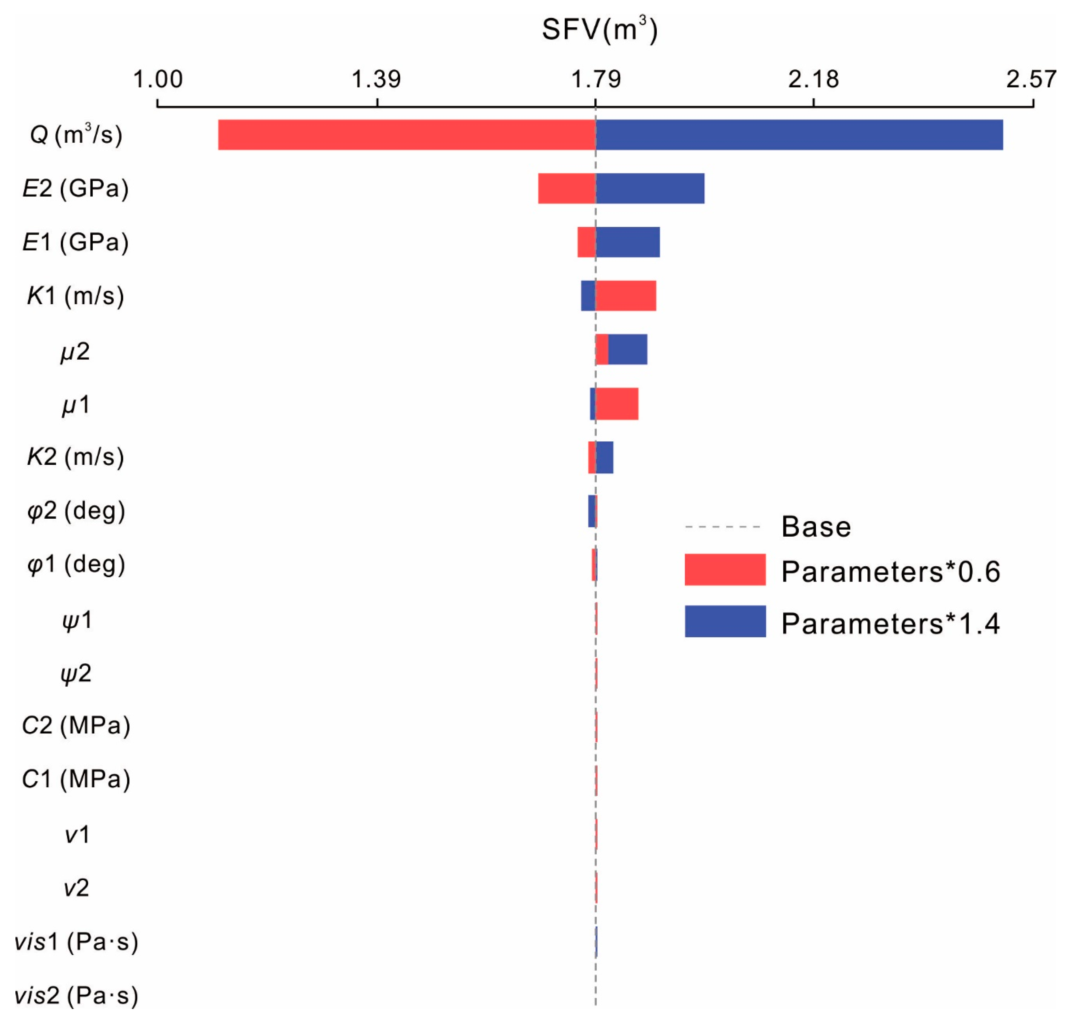
Figure 8.
Coefficients referred to coded parameters and their standard errors. (a) Coefficient estimates of single factors and (b) coefficient estimates of joint action parameters.
Figure 8.
Coefficients referred to coded parameters and their standard errors. (a) Coefficient estimates of single factors and (b) coefficient estimates of joint action parameters.

Figure 9.
Statistical significance of variables and their joint action to SRV.
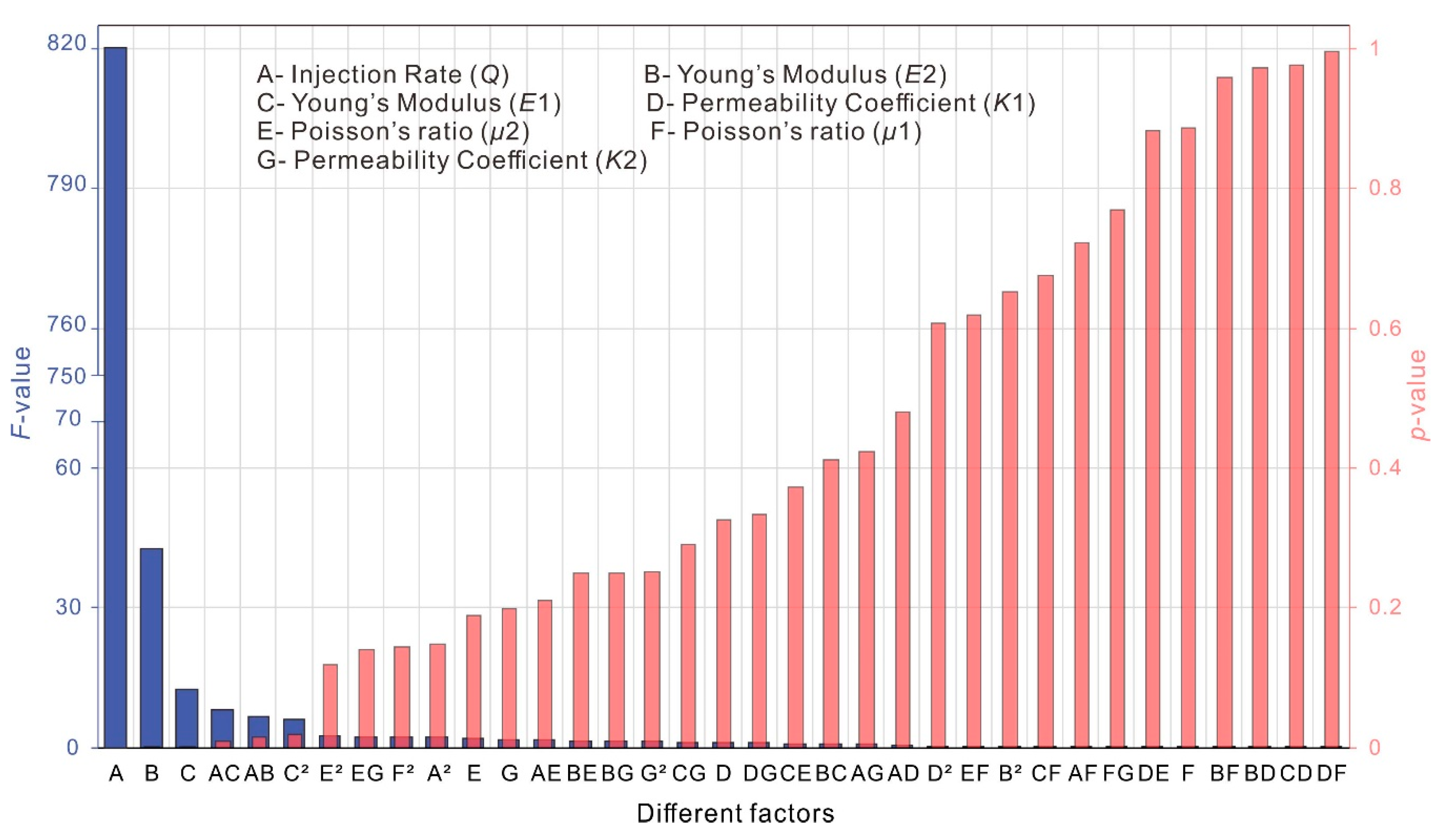
Figure 10.
The cross plot of actual value against the predicted value of SRV.
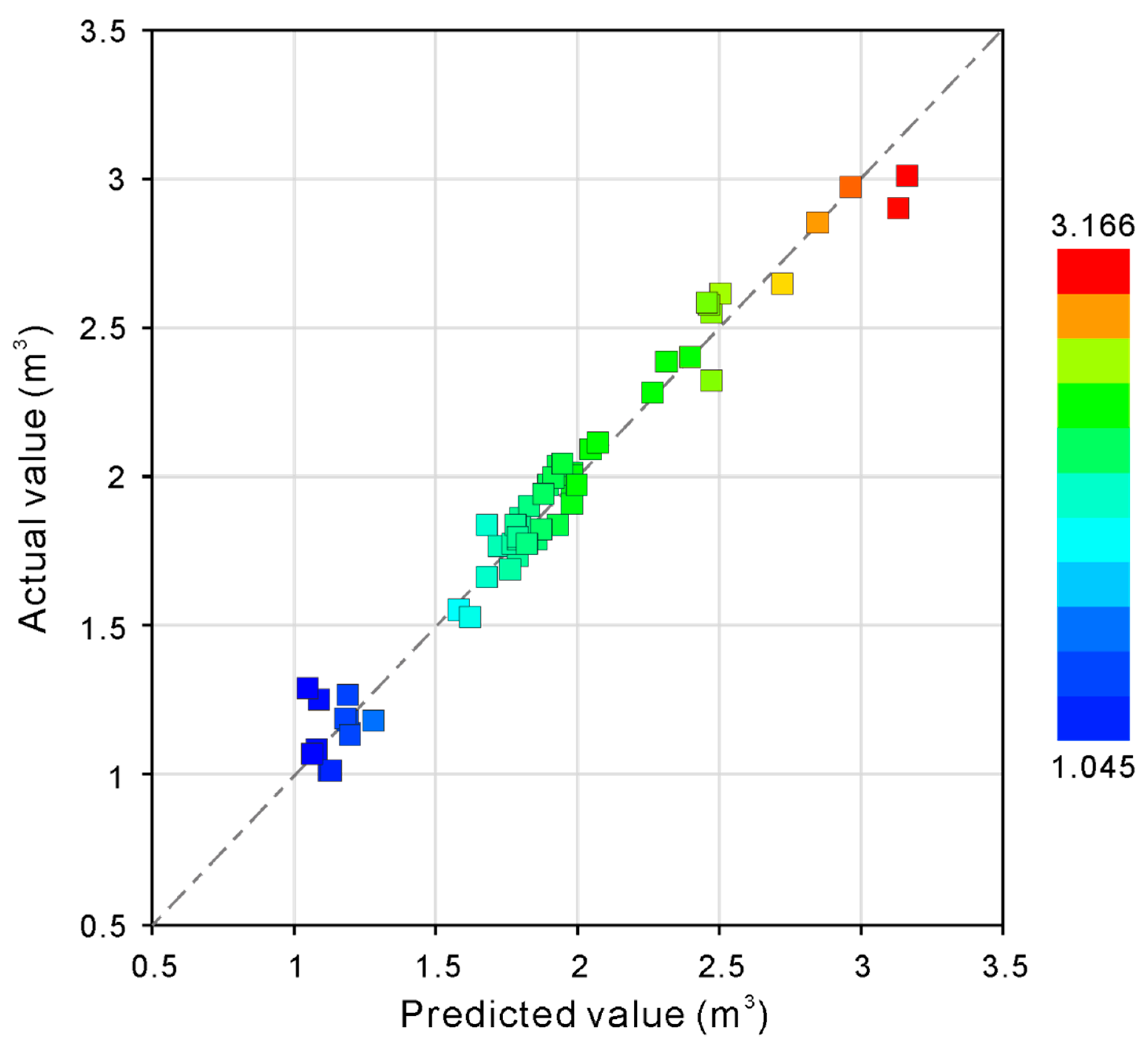
Figure 11.
Fracture morphology, SRV, and breakdown pressure under different injection rates Q. (a) Profiles of fracture considering different Q; (b) SRV and breakdown pressure under different Q.
Figure 11.
Fracture morphology, SRV, and breakdown pressure under different injection rates Q. (a) Profiles of fracture considering different Q; (b) SRV and breakdown pressure under different Q.

Figure 12.
Fracture morphology, SRV, and breakdown pressure under different Young’s modulus. (a) Profiles of fractures under different reservoir Young’s modulus E1; (b) SRV and breakdown pressure under different E1; (c) profiles of fracture under different barrier Young’s modulus E2; (d) SRV and breakdown pressure under different E2.
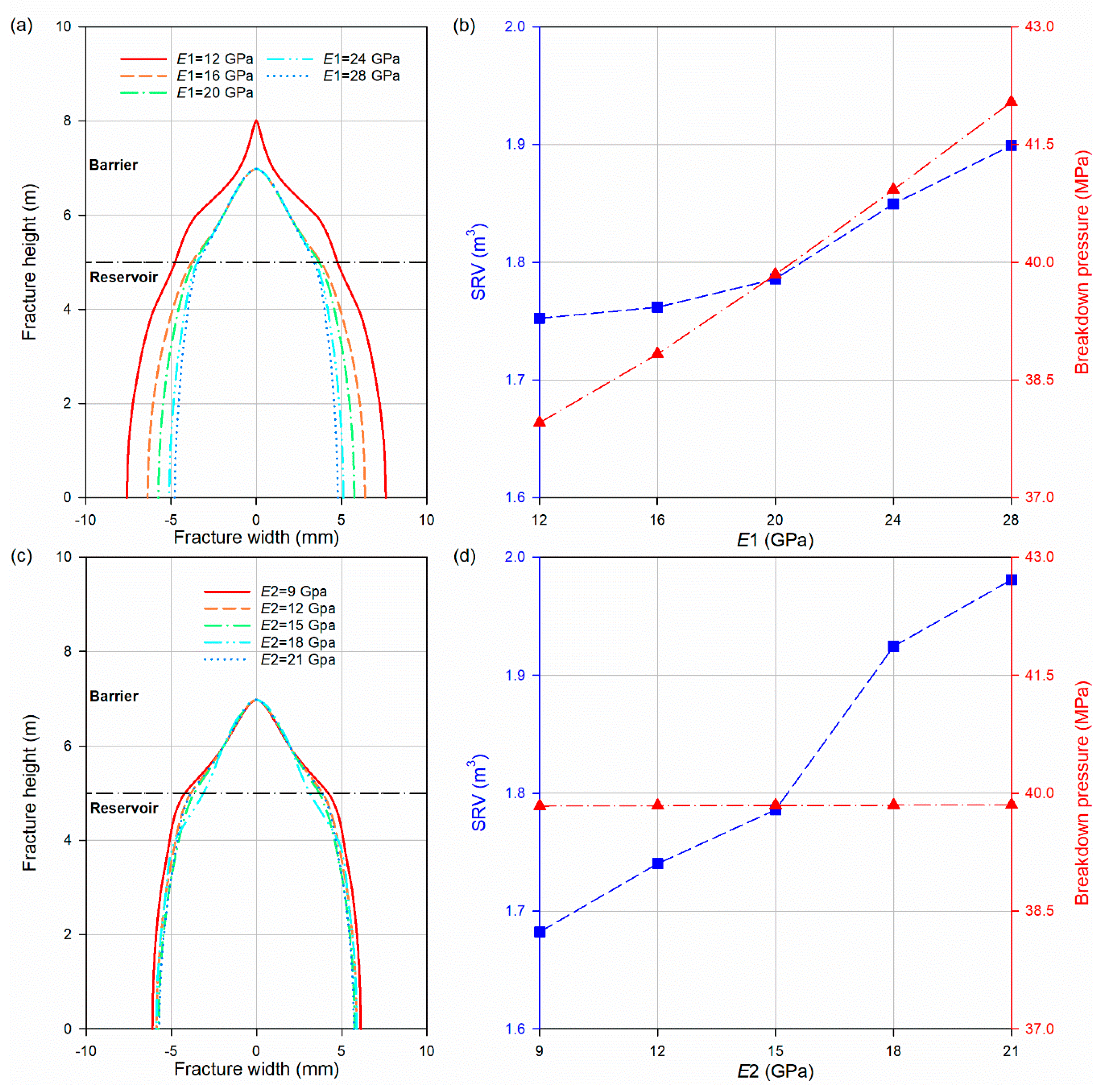
Figure 13.
Response surface of the interaction between E1 and E2 to SRV.

Figure 14.
Fracture morphology, SRV, and breakdown pressure under different Poisson’s ratios. (a) Profiles of fractures under different reservoir Poisson’s ratio μ1; (b) SRV and breakdown pressure under different μ1; (c) profiles of fractures under different barrier Poisson’s ratio μ2; (d) SRV and breakdown pressure under different μ2.

Figure 15.
Response surface of the interaction between μ1 and μ2 to SRV.
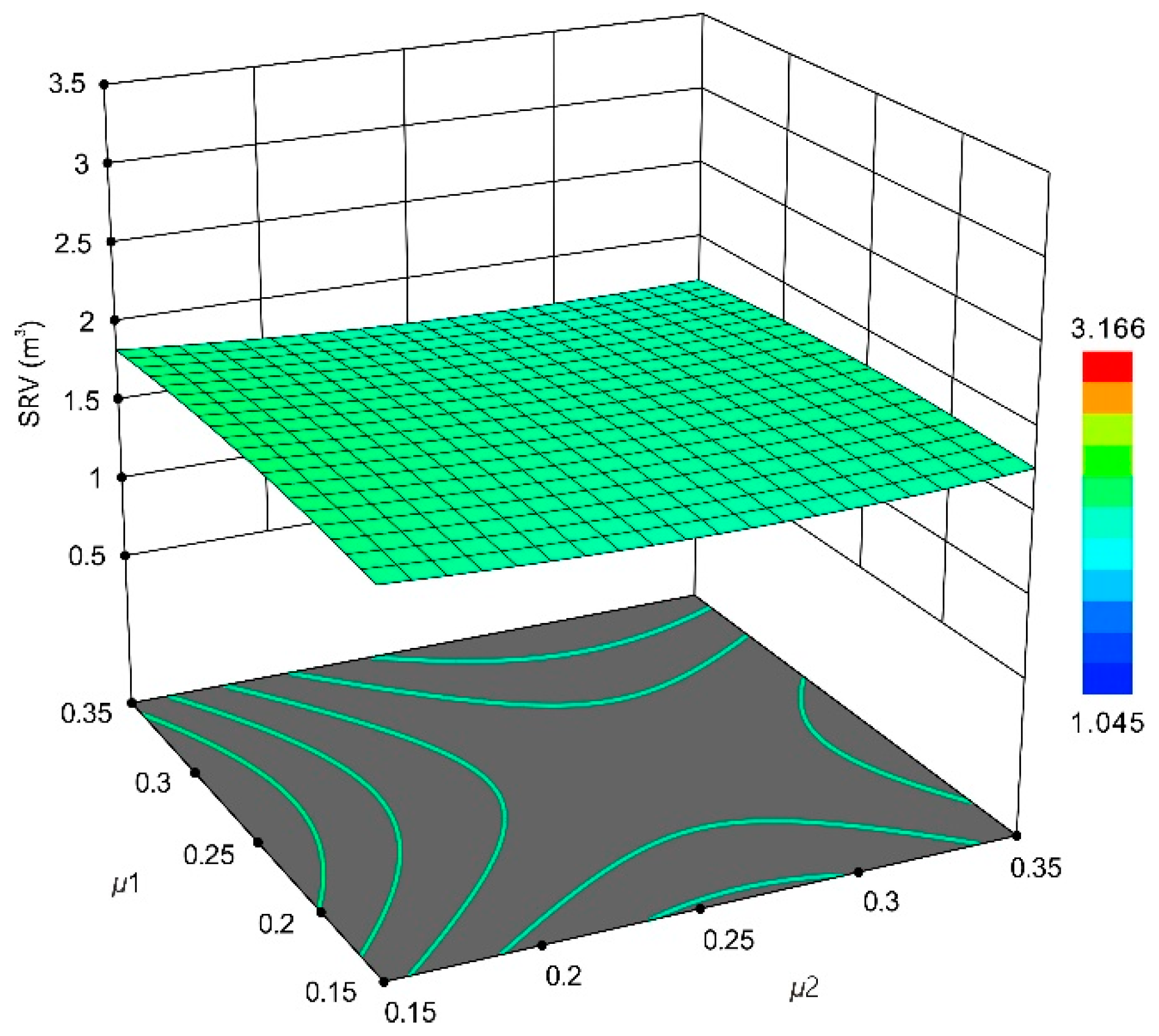
Figure 16.
Fracture morphology, SRV, and breakdown pressure under different permeability coefficients. (a) Profiles of fractures under different reservoir permeability coefficient K2; (b) SRV and breakdown pressure under different K1; (c) profiles of fractures under different barrier permeability coefficient K2; (d) SRV and breakdown pressure under different K2.
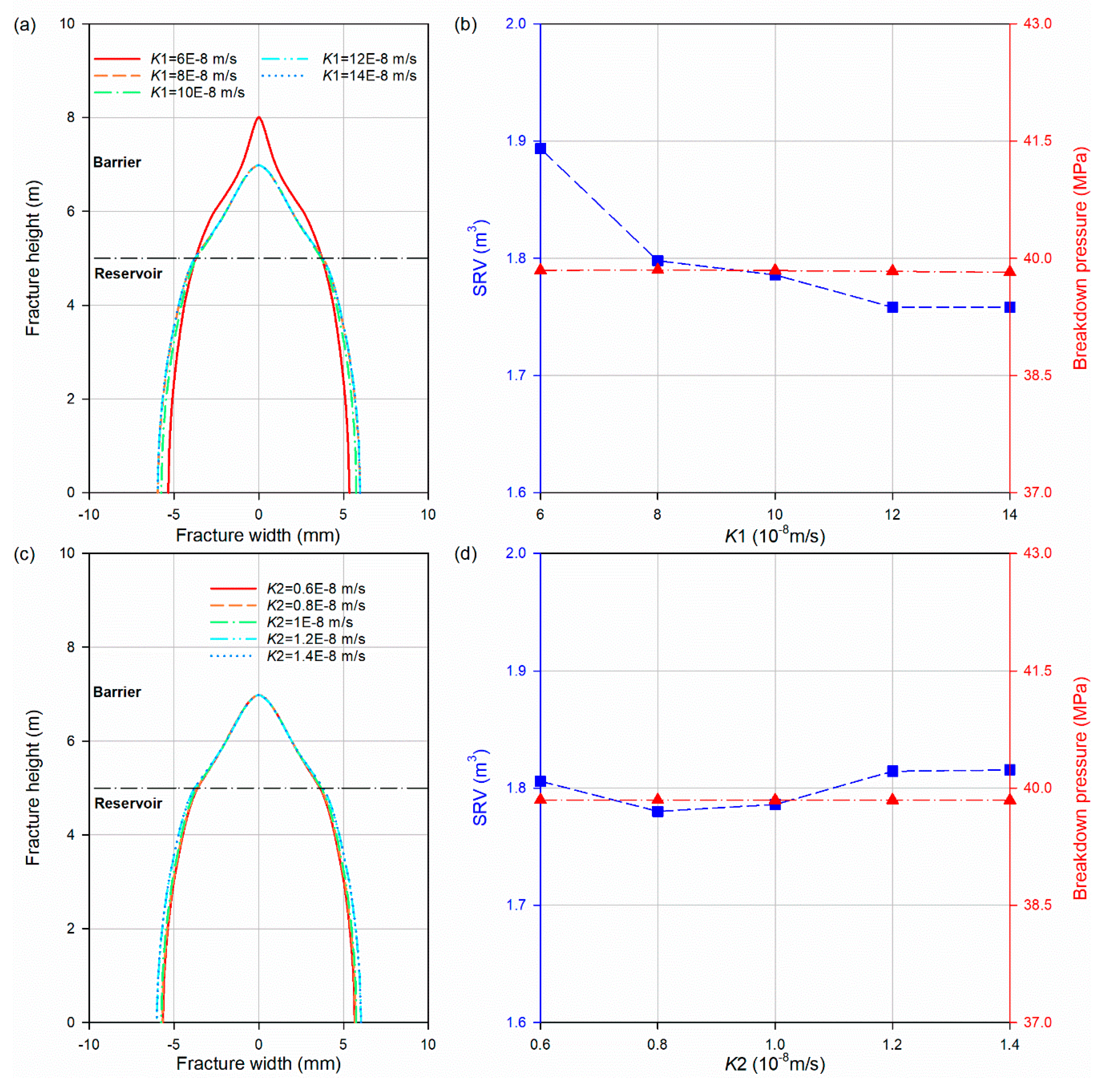
Figure 17.
Response surface of the interaction between K1 and K2 to SRV.

Table 1.
Underlying parameters used in the numerical analysis.
| Parameter | Reservoir | Barrier | Unit |
|---|---|---|---|
| Young’s modulus | 20 | 15 | GPa |
| Poisson’s ratio | 0.25 | 0.25 | - |
| Friction angle | 25 | 30 | deg |
| Cohesion | 11 | 8 | MPa |
| Dilatancy angle | 20 | 25 | deg |
| Initial permeability | 1.0 10−7 | 1.0 10−8 | m/s |
| Void ratio | 0.2 | 0.2 | - |
Table 2.
Multiple parameters for experimental design.
| Stratum | Parameters | Maximum | Median (Benchmark) | Minimum | Unit |
|---|---|---|---|---|---|
| Reservoir | Injection rate (Q) | 0.014 | 0.001 | 0.006 | m3/s |
| Young’s modulus (E1) | 28 | 20 | 12 | GPa | |
| Poisson’s ratio (μ1) | 0.35 | 0.25 | 0.15 | - | |
| Friction angle (φ1) | 35 | 25 | 15 | deg | |
| Cohesion (C1) | 15.4 | 11 | 6.6 | MPa | |
| Permeability coefficient (K1) | 14 | 10 | 6 | 10−8 m/s | |
| Void ratio (ν1) | 0.28 | 0.2 | 0.12 | - | |
| Dilatancy angle (ψ1) | 28 | 20 | 12 | deg | |
| Viscosity (vis1) | 0.0014 | 0.001 | 0.0006 | Pa·s | |
| Barrier | Young’s modulus (E2) | 21 | 15 | 9 | GPa |
| Poisson’s ratio (μ2) | 0.35 | 0.25 | 0.15 | - | |
| Friction angle (φ2) | 42 | 30 | 18 | deg. | |
| Cohesion (C2) | 11.2 | 8 | 4.8 | MPa | |
| Permeability coefficient (K2) | 1.4 | 1 | 0.6 | 10−8 m/s | |
| Void ratio (ν2) | 0.28 | 0.2 | 0.12 | - | |
| Dilatancy angle (ψ2) | 35 | 25 | 15 | deg | |
| Viscosity (vis2) | 0.0014 | 0.001 | 0.006 | Pa·s |
Table 3.
The results of the Box–Behnken experiment.
| Run | Factor A: | Factor B: | Factor C: | Factor D: | Factor E: | Factor F: | Factor G: | SRV |
|---|---|---|---|---|---|---|---|---|
| Q (m3/s) | E2 (GPa) | E1 (GPa) | K1 (10−8 m/s) | μ2 | μ1 | K2 (10−8 m/s) | (m3) | |
| 1 | 0.01 | 15 | 20 | 10 | 0.25 | 0.25 | 1 | 1.786 |
| 2 | 0.01 | 21 | 28 | 10 | 0.25 | 0.15 | 1 | 2.048 |
| 3 | 0.01 | 9 | 20 | 10 | 0.15 | 0.25 | 0.6 | 1.723 |
| 4 | 0.01 | 15 | 12 | 14 | 0.25 | 0.25 | 1.4 | 1.928 |
| 5 | 0.01 | 15 | 12 | 6 | 0.25 | 0.25 | 0.6 | 1.978 |
| 6 | 0.006 | 9 | 20 | 6 | 0.25 | 0.25 | 1 | 1.081 |
| 7 | 0.01 | 15 | 20 | 10 | 0.25 | 0.25 | 1 | 1.786 |
| 8 | 0.014 | 15 | 20 | 10 | 0.25 | 0.35 | 1.4 | 2.474 |
| 9 | 0.01 | 21 | 20 | 10 | 0.15 | 0.25 | 1.4 | 1.982 |
| 10 | 0.006 | 15 | 20 | 10 | 0.25 | 0.15 | 1.4 | 1.115 |
| 11 | 0.01 | 15 | 20 | 6 | 0.35 | 0.15 | 1 | 1.85 |
| 12 | 0.01 | 21 | 20 | 10 | 0.35 | 0.25 | 0.6 | 1.978 |
| 13 | 0.01 | 9 | 12 | 10 | 0.25 | 0.35 | 1 | 1.582 |
| 14 | 0.014 | 15 | 28 | 10 | 0.15 | 0.25 | 1 | 3.166 |
| 15 | 0.01 | 9 | 12 | 10 | 0.25 | 0.15 | 1 | 1.621 |
| 16 | 0.014 | 9 | 20 | 14 | 0.25 | 0.25 | 1 | 2.395 |
| 17 | 0.006 | 15 | 12 | 10 | 0.35 | 0.25 | 1 | 1.083 |
| 18 | 0.01 | 9 | 20 | 10 | 0.35 | 0.25 | 1.4 | 1.675 |
| 19 | 0.01 | 15 | 20 | 6 | 0.35 | 0.35 | 1 | 1.787 |
| 20 | 0.006 | 15 | 28 | 10 | 0.15 | 0.25 | 1 | 1.193 |
| 21 | 0.006 | 21 | 20 | 14 | 0.25 | 0.25 | 1 | 1.19 |
| 22 | 0.01 | 9 | 20 | 10 | 0.15 | 0.25 | 1.4 | 1.682 |
| 23 | 0.01 | 9 | 20 | 10 | 0.35 | 0.25 | 0.6 | 1.678 |
| 24 | 0.01 | 15 | 12 | 6 | 0.25 | 0.25 | 1.4 | 1.759 |
| 25 | 0.01 | 15 | 20 | 14 | 0.35 | 0.35 | 1 | 1.768 |
| 26 | 0.014 | 15 | 28 | 10 | 0.35 | 0.25 | 1 | 3.137 |
| 27 | 0.014 | 15 | 20 | 10 | 0.25 | 0.15 | 1.4 | 2.507 |
| 28 | 0.006 | 21 | 20 | 6 | 0.25 | 0.25 | 1 | 1.178 |
| 29 | 0.01 | 15 | 20 | 10 | 0.25 | 0.25 | 1 | 1.786 |
| 30 | 0.01 | 15 | 28 | 6 | 0.25 | 0.25 | 0.6 | 1.928 |
| 31 | 0.01 | 21 | 20 | 10 | 0.15 | 0.25 | 0.6 | 2.472 |
| 32 | 0.014 | 15 | 20 | 10 | 0.25 | 0.35 | 0.6 | 2.459 |
| 33 | 0.006 | 15 | 20 | 10 | 0.25 | 0.35 | 0.6 | 1.278 |
| 34 | 0.006 | 15 | 28 | 10 | 0.35 | 0.25 | 1 | 1.184 |
| 35 | 0.014 | 15 | 20 | 10 | 0.25 | 0.15 | 0.6 | 2.456 |
| 36 | 0.014 | 21 | 20 | 14 | 0.25 | 0.25 | 1 | 2.962 |
| 37 | 0.01 | 15 | 20 | 14 | 0.35 | 0.15 | 1 | 1.872 |
| 38 | 0.014 | 15 | 12 | 10 | 0.15 | 0.25 | 1 | 2.718 |
| 39 | 0.01 | 15 | 20 | 10 | 0.25 | 0.25 | 1 | 1.786 |
| 40 | 0.01 | 15 | 20 | 14 | 0.15 | 0.15 | 1 | 1.797 |
| 41 | 0.01 | 15 | 28 | 6 | 0.25 | 0.25 | 1.4 | 1.896 |
| 42 | 0.006 | 15 | 12 | 10 | 0.15 | 0.25 | 1 | 1.045 |
| 43 | 0.01 | 9 | 28 | 10 | 0.25 | 0.15 | 1 | 1.795 |
| 44 | 0.006 | 15 | 20 | 10 | 0.25 | 0.35 | 1.4 | 1.129 |
| 45 | 0.014 | 21 | 20 | 6 | 0.25 | 0.25 | 1 | 2.847 |
| 46 | 0.014 | 15 | 12 | 10 | 0.35 | 0.25 | 1 | 2.313 |
| 47 | 0.006 | 9 | 20 | 14 | 0.25 | 0.25 | 1 | 1.061 |
| 48 | 0.01 | 15 | 20 | 14 | 0.15 | 0.35 | 1 | 1.825 |
| 49 | 0.01 | 21 | 20 | 10 | 0.35 | 0.25 | 1.4 | 1.999 |
| 50 | 0.01 | 15 | 12 | 14 | 0.25 | 0.25 | 0.6 | 1.976 |
| 51 | 0.01 | 21 | 12 | 10 | 0.25 | 0.35 | 1 | 1.994 |
| 52 | 0.006 | 15 | 20 | 10 | 0.25 | 0.15 | 0.6 | 1.194 |
| 53 | 0.014 | 9 | 20 | 6 | 0.25 | 0.25 | 1 | 2.261 |
| 54 | 0.01 | 15 | 28 | 14 | 0.25 | 0.25 | 0.6 | 1.914 |
| 55 | 0.01 | 15 | 20 | 10 | 0.25 | 0.25 | 1 | 1.786 |
| 56 | 0.01 | 15 | 20 | 10 | 0.25 | 0.25 | 1 | 1.786 |
| 57 | 0.01 | 15 | 28 | 14 | 0.25 | 0.25 | 1.4 | 2.067 |
| 58 | 0.01 | 21 | 28 | 10 | 0.25 | 0.35 | 1 | 1.942 |
| 59 | 0.01 | 15 | 20 | 6 | 0.15 | 0.35 | 1 | 1.776 |
| 60 | 0.01 | 21 | 12 | 10 | 0.25 | 0.15 | 1 | 1.882 |
| 61 | 0.01 | 15 | 20 | 6 | 0.15 | 0.15 | 1 | 1.789 |
| 62 | 0.01 | 9 | 28 | 10 | 0.25 | 0.35 | 1 | 1.822 |
© 2019 by the authors. Licensee MDPI, Basel, Switzerland. This article is an open access article distributed under the terms and conditions of the Creative Commons Attribution (CC BY) license (http://creativecommons.org/licenses/by/4.0/).
Share and Cite
MDPI and ACS Style
Zhang, J.; Liu, X.; Wei, X.; Liang, L.; Xiong, J.; Li, W. Uncertainty Analysis of Factors Influencing Stimulated Fracture Volume in Layered Formation. Energies 2019, 12, 4444. https://doi.org/10.3390/en12234444
AMA Style
Zhang J, Liu X, Wei X, Liang L, Xiong J, Li W. Uncertainty Analysis of Factors Influencing Stimulated Fracture Volume in Layered Formation. Energies. 2019; 12(23):4444. https://doi.org/10.3390/en12234444
Chicago/Turabian StyleZhang, Jingxuan, Xiangjun Liu, Xiaochen Wei, Lixi Liang, Jian Xiong, and Wei Li. 2019. "Uncertainty Analysis of Factors Influencing Stimulated Fracture Volume in Layered Formation" Energies 12, no. 23: 4444. https://doi.org/10.3390/en12234444
Note that from the first issue of 2016, this journal uses article numbers instead of page numbers. See further details here.