Prediction of Hydropower Generation Using Grey Wolf Optimization Adaptive Neuro-Fuzzy Inference System

Abstract

Hydropower is among the cleanest sources of energy. However, the rate of hydropower generation is profoundly affected by the inflow to the dam reservoirs. In this study, the Grey wolf optimization (GWO) method coupled with an adaptive neuro-fuzzy inference system (ANFIS) to forecast the hydropower generation. For this purpose, the Dez basin average of rainfall was calculated using Thiessen polygons. Twenty input combinations, including the inflow to the dam, the rainfall and the hydropower in the previous months were used, while the output in all the scenarios was one month of hydropower generation. Then, the coupled model was used to forecast the hydropower generation. Results indicated that the method was promising. GWO-ANFIS was capable of predicting the hydropower generation satisfactorily, while the ANFIS failed in nine input-output combinations.

1. Introduction

Hydropower is a renewable source of energy that is derived from the fast reservoir water flows through a turbine. One of the main purposes of dam construction is to generate the hydropower via installation of a hydropower plant near the dam site. The rate of hydropower generation depends on the dam height and the inflow to the dam reservoir. Nonetheless, hydropower is one of the major sources of power supply in each country. In addition, the power consumption varies strongly during the year. Therefore, an insight on the value of hydropower energy to be produced in the coming months would be an important tool in managing the electricity distribution network and operation of the dam. Consequently, hydropower generation forecasting could be a key component in dam operation. Hamlet et al. [1] evaluated a long-lead forecasting model in the Colombia river and stated that long-lead forecasting model led to an increase in annual revenue of approximately $153 million per year in comparison with no forecasting model. Several researches carried out based on the inflow forecasting to the dam and executing an operating reservoir model to determine the hydropower generation [2,3,4,5,6,7,8]. While these researches are promising, some challenges arise during the implementation of these models. First, forecasting the precipitation is needed and in the next step the inflow to the river and then a reservoir model needs to be run. Each step, including the precipitation or inflow forecasting and reservoir modeling, is associated with uncertainty and the results are highly affected by the uncertainty in these models. Second, an optimization algorithm seems to be needed to optimize the parameters of predictive models.

During the past two decades, several artificial intelligent models were utilized for hydrologic model prediction [9] and hydropower stream flow forecasting [10]. Among them, the ensemble models [11,12,13] and hybrid models [14] have recently become very popular. Recently, to produce novel hybrid models, different optimization algorithms were coupled with these models to improve their performance [15,16,17,18,19,20]. Among the optimization algorithms, Grey wolf optimization (GWO) has shown promising results in a wide range of application when coupled with machine learning algorithms [21]. Consequently, in this study, to reduce the source of uncertainty, an artificial intelligent model was used for hydropower generation forecasting. For this purpose, the adaptive neuro-fuzzy inference system (ANFIS) was coupled with GWO to forecast the monthly hydropower generation directly based on the precipitation over the basin, the inflow to the dam and the hydropower generation in previous months. This method is capable to facilitate the hydropower generation forecasting. The rest of this chapter is organized as follows. In Section 2, the coupled model of ANFIS and GWO and study area are presented. Section 3 involves the results of hydropower forecasting and its reliability. Finally, Section 4 includes the conclusion of the study.

2. Methodology and Data

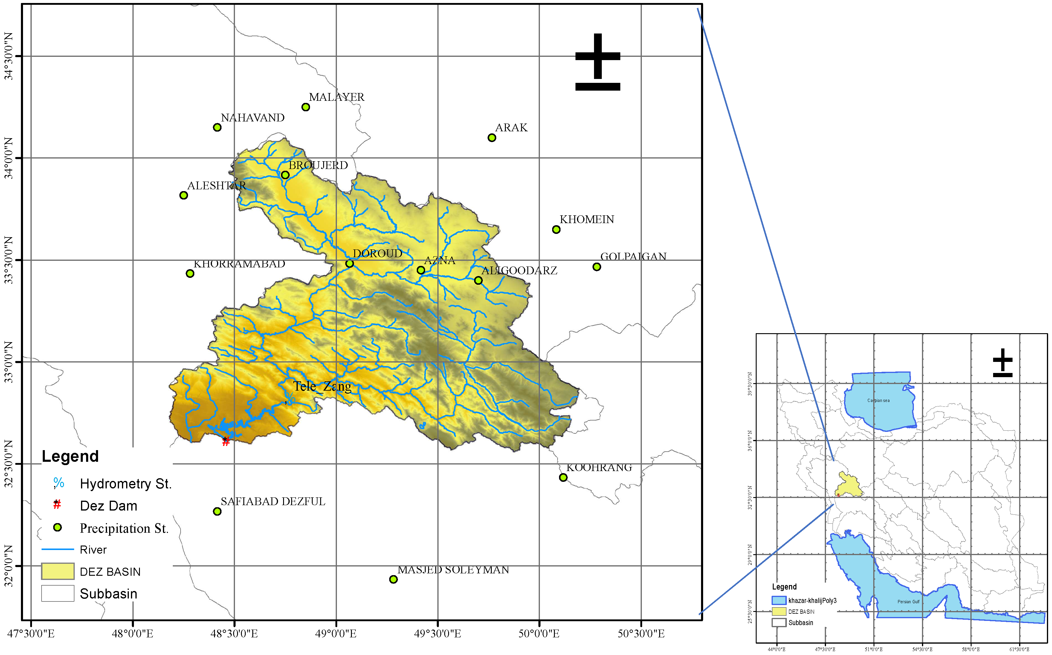
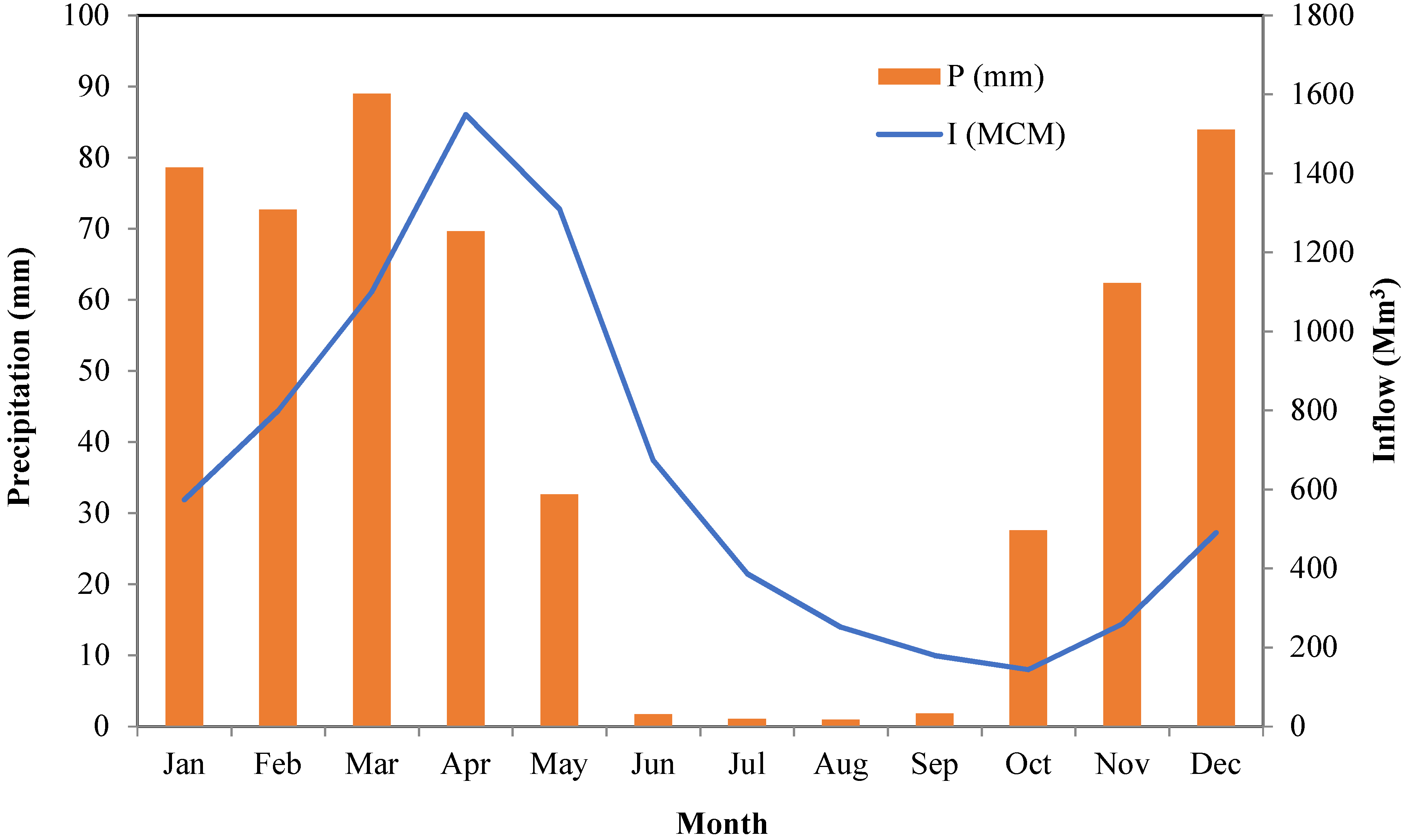
2.1. Study Area

The Dez dam is an arch dam constructed in 1963 on the Dez river southwestern of Iran (Figure 1). The dam is 203 m high and has a reservoir capacity of 3340 Mm³. The upstream catchment of the dam with the mean elevation of 1915.3 m above sea level and average slope of 0.0084 has an area of 17,843.3 Km². The catchment length is about 400 km and ends with the dam reservoir at the outlet. Flow to the reservoir was measured at the Tele-Zang hydrometric station (Figure 1). The precipitation stations that were used in the present study include four precipitation stations in the catchment and 10 others around the catchment (Figure 1). The hydrometric data was taken from Iran’s Water Resources Management Company (http://www.wrm.ir/index.php?l=EN) and the precipitation data is available from Iran Meteorological Organization (http://www.irimo.ir/eng/index.php). The monthly data used here covered the range of October 1963 to September 2017. The average Inflow to the reservoir and precipitation were calculated and shown in Figure 2. According to Figure 2, the most precipitation occurred from October to May. Precipitation in the winter accumulated as snowpack over the high mountainous area and in the spring the river flow increased as a result of snowmelt. Summer was dry with almost no considerable precipitation.

The primary purpose of the Dez dam is the flood control, hydroelectric power generation and irrigation supply for 125,000 ha downstream agricultural area, as well. The Dez hydropower plant consists of eight units with a total installed capacity of 520 MW. The monthly power generation was gathered between 1963 and 2017 from Iran’s Water Resources Management Company. Figure 3 illustrates monthly hydroelectric generation in the Dez hydropower plant.

Table 1. Presenting the datasets and the statistical characteristics.

Parameter	Mode	Mean	Min	S.D.	First Quartile	Median	Third Quartile	Max	Skew.	Kurtosis.
Ht	26,545.98	165,297.70	26,545.98	56,093.06	130,338.42	168,568.96	203,734.07	354,879.53	−0.10	2.76
Qt	63.28	651.71	63.28	615.23	209.87	430.22	842.41	3643.84	1.86	6.91
Pt	0.00	42.82	0.00	46.91	0.47	27.97	71.81	238.47	1.10	3.69

Ht: Hydroelectric Energy (MWH) at month t; Qt: River Inflow (m³/s) at month t; Pt: precipitation (mm) at month t; S.D.: Standard Deviation.

shows the statistical characteristics of the precipitation over the Dez basin, the inflow to the dam reservoir and the hydropower generation time series.

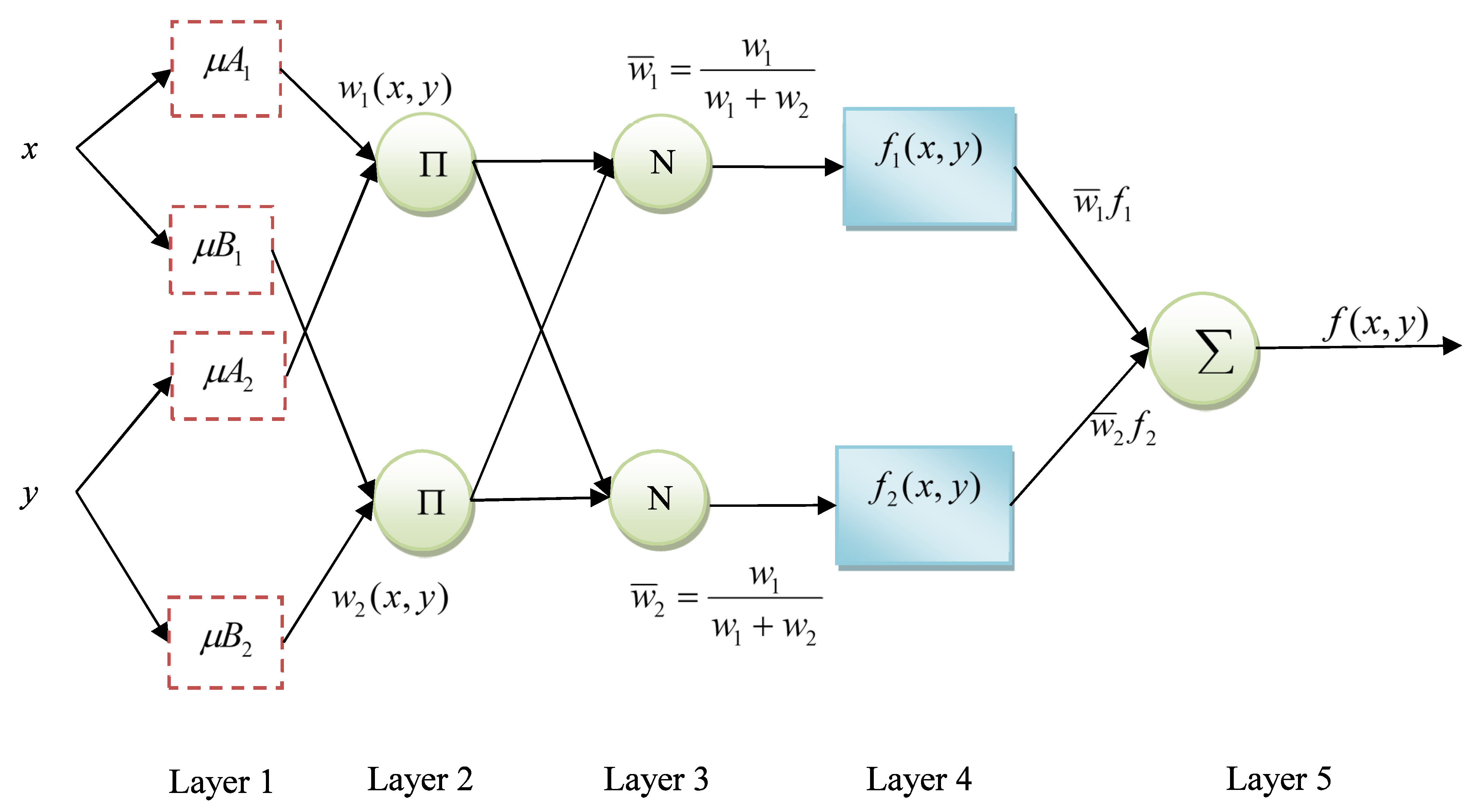
2.2. ANFIS: Adaptive Neuro-Fuzzy Inference System

Jang (1993) [22] developed ANFIS as a joint of artificial neural network and the fuzzy inference system [23]. The learning ability of artificial neural networks (ANN) and the fuzzy reasoning create a valuable capability to fit a relationship between input and output spaces [24]. On the other hand, the ANFIS uses the training capability of ANN to assign and adjust the membership functions. The back-propagation algorithm enables the model to adjust the parameters until an acceptable error is reached [25]. Suppose that the system of fuzzy inference include x & y as inputs and z as output. Two if-then rules could be utilized for Sugeno model as follows:

• Rule one: if x and y = $A_1$ and $B_1$, respectively, then $f_1=p_{1}x+q_{1}y+r_1$.
• Rule two: if x and y =$A_2$ and $B_2$, respectively, then $f_2=p_{2}x+q_{2}y+r_2$

where $A_1$, $B_1$, $A_2$, $B_2$ are considered as the labels of linguistic. Furthermore, $p_1$, $p_2$, $q_1$, $q_2$, $r_1$ and $r_2$ are the output function parameters [26].

The architecture of ANFIS is presented in Figure 4. It includes five layers; all are fixed nodes, except the first and fourth nodes, which are adaptive nodes.

Layer 1: The nodes act adaptive in generating the membership grades of the inputs [24]:

$$\begin{array}{c}{O}_{1,i}={\mu }_{Ai}(x),\mathrm{for}i=1,2,\mathrm{or}\\ O_{1,i}={\mu }_{Bi-2}(y),\mathrm{for}i=3,4.\end{array}$$

(1)

It should be noted that i is the number of inputs and $O_{1,i}$ to $O_{5,i}$ are the output of each layer. Several memberships could be used for this purpose; among all Gaussian functions presented in the Equation (1), the following was utilized in this study:

$$\mu \left(x\right)=\exp \left[-0.5{\left\{\frac{x-c_i}{{\sigma }_i}\right\}}^2\right]$$

(2)

where $c_i$ and ${\sigma }_i$ are set parameters with maximum and minimum of one and zero, respectively [22].

Layer 2: this layer is a rule node with AND/OR operator to get an output which called firing strengths $O_{2,i}$:

$$O_{2,i}={\mu }_{Ai}(x){\mu }_{Bi}(y),i=1,2$$

(3)

Layer 3: presents an average node computing the normalized firing strength as follows:

$$O_{3,i}={\overline{w}}_i=\frac{w_i}{w_1+w_2},i=1,2$$

(4)

Layer 4: this layer contains the consequent nodes for which the$p$, $q$ and $r$ parameters were tuned during the learning process:

$$O_{4,i}={\overline{w}}_i{f}_i={\overline{w}}_i(p_{i}x+q_{i}y+r_i)$$

(5)

Layer 5: this layer contains the output nodes which compute the total average of output through a sum of entire input signals [27]:

$$O_{5,i}=f={\displaystyle \sum _i{\overline{w}}_i{f}_i}$$

(6)

While the ANFIS has high capability to map the input to the output as a black-box model, it suffers from a long training time to assign the proper values to the parameters of membership function. To overcome this problem we use the optimization algorithm of grey wolf.

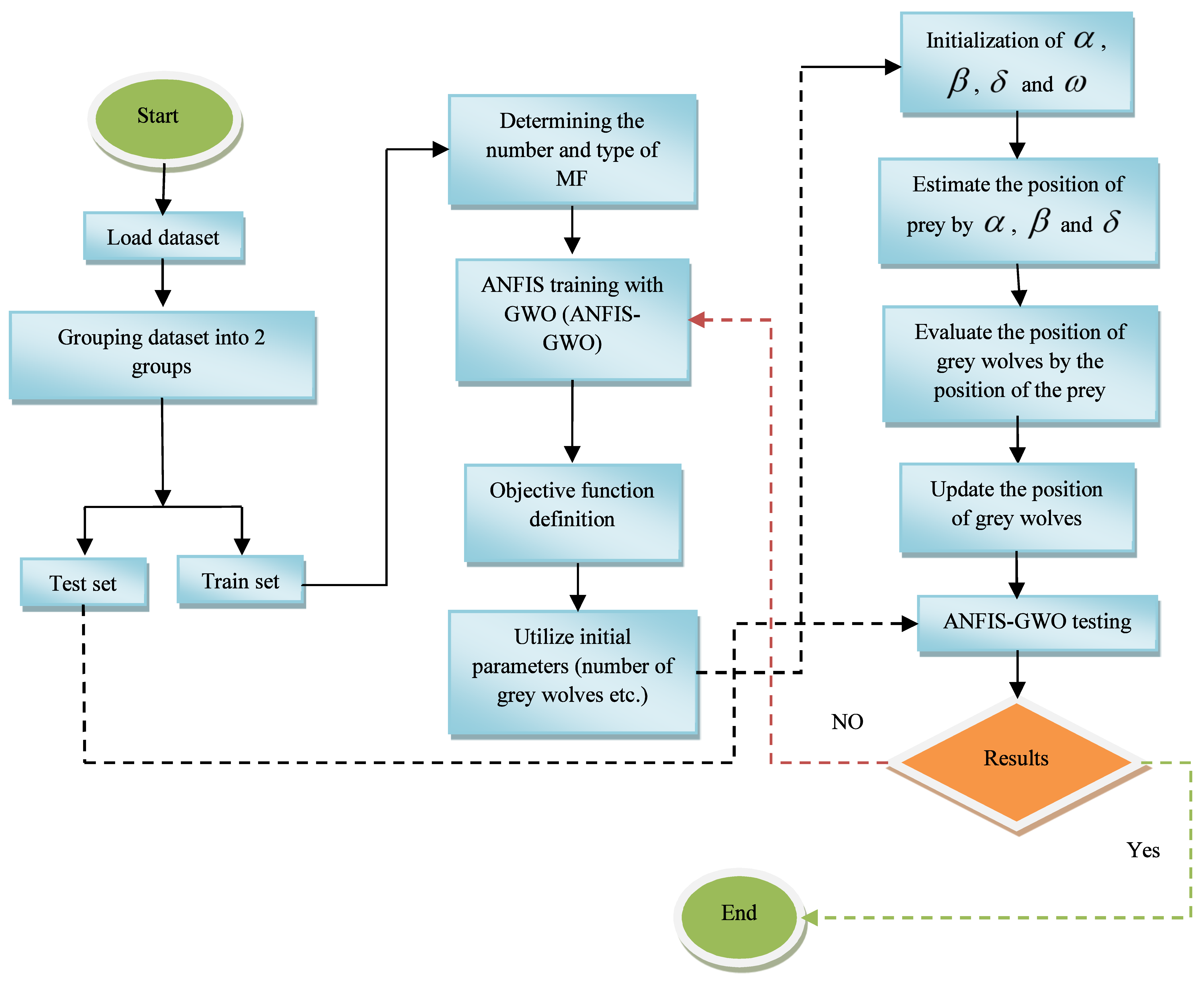
2.3. Grey Wolf Optimization (GWO)

The optimization algorithm of Grey wolf known as GWO is known as an advanced meta-heuristic nature-inspired for an efficient optimization [28]. This algorithm was developed through imitating the foraging behavior of grey wolfs performing in groups of five-12 individuals which are at the top of food chain [29]. Grey wolves follow a social hierarchy strictly.

The leaders include a couple of female and male, called alpha ($\alpha$), who are in charge of decision making while hunting, resting and so on. Beta ($\beta$) is the next level helping alpha in making decisions, while they should obey the alpha. The beta wolves can be male and female and the role of them is disciplining the group. They are the best candidate for substituting the alpha when they become older or die. The next level is called delta ($\delta$) and play the role of scouts, sentinels, hunters and so on. The last level is called omega ($\omega$), which are the weakest level. They act as babysitters. While this level is the weakest, without omega wolves, internal fights may be observed in the group. Hunting, along with the social hierarchy, is a major social behavior of grey wolves. Muro et al. [30] expressed the three steps in the grey wolves hunting:

• Identifying, following and approaching the prey;
• Encircling the prey;
• Attacking the prey.

These two social behaviors are considered in the GWO algorithm [29]. In mathematical modeling of the algorithm, $\alpha$ is considered as the fittest solution, and in the next steps, $\beta$, $\delta$ and $\omega$. The mathematical formulation of encircling could be presented as follows [28]:

$$\overrightarrow{D}=\left|\overrightarrow{C}\cdot {\overrightarrow{X}}_p(t)-\overline{X}(t)\right|$$

(7)

$$\overrightarrow{X}(t+1)={\overrightarrow{X}}_p(t)-\overrightarrow{A}\cdot \overrightarrow{D}$$

(8)

where, $\overrightarrow{A}$ and $\overrightarrow{C}$ would work as the vectors of the coefficient. Furthermore, $\overrightarrow{X_p}$ would determine the positions of prey and $\overrightarrow{X}$ is the wolf's positions. Here, $\overrightarrow{D}$ would be the vector for specifying a new position of the GW and $t$ is the iteration time. The $\overrightarrow{C}$ and $\overrightarrow{A}$ formulated as [28]:

$$\overrightarrow{A}=2\overrightarrow{a}\cdot \overrightarrow{r_1}-\overrightarrow{a}$$

(9)

$$\overrightarrow{C}=2\cdot \overrightarrow{r_2}$$

(10)

where $\overrightarrow{a}$ presents the set of vectors over the iteration that change in value from 2 to 0 linearly. The $\overrightarrow{r_1}$ and $\overrightarrow{r_2}$ represent random vectors in $[0,1]$.

The$\alpha$ leads the hunting, while $\beta$ and $\delta$contribute in this task occasionally. For mathematical representation of hunting, it was assumed that the alpha, bata and delta include better knowledge on the prey’s locations. Thus, the optimal solutions for the three positions can be registered. Consequently, the rest of the wolves will follow and update their postions accordingly.

$${\overrightarrow{D}}_{\alpha }=\left|{\overrightarrow{C}}_1\cdot {\overrightarrow{X}}_{\alpha }-\overrightarrow{X}\right|$$

(11)

$${\overrightarrow{D}}_{\beta }=\left|{\overrightarrow{C}}_2\cdot {\overrightarrow{X}}_{\beta }-\overrightarrow{X}\right|$$

(12)

$${\overrightarrow{D}}_{\delta }=\left|{\overrightarrow{C}}_3\cdot {\overrightarrow{X}}_{\delta }-\overrightarrow{X}\right|$$

(13)

$${\overrightarrow{X}}_1={\overrightarrow{X}}_{\alpha }-A_1\cdot {\overrightarrow{D}}_{\alpha }$$

(14)

$${\overrightarrow{X}}_2={\overrightarrow{X}}_{\beta }-A_2\cdot {\overrightarrow{D}}_{\beta }$$

(15)

$${\overrightarrow{X}}_3={\overrightarrow{X}}_{\delta }-A_3\cdot {\overrightarrow{D}}_{\delta }$$

(16)

$$\overrightarrow{X}(t+1)=\frac{{\overrightarrow{X}}_1+{\overrightarrow{X}}_2+{\overrightarrow{X}}_3}{3}$$

(17)

When the prey stops, the grey wolves start to attack. The vector $A$ is a random value in the interval$[-2a,2a]$. The $\left|A\right|<1$ leads to grey wolves’ attack while $\left|A\right|>1$ force them to move away to find a better solution. Figure 5 shows the framework of the GWO algorithm.

2.4. Performance Criteria

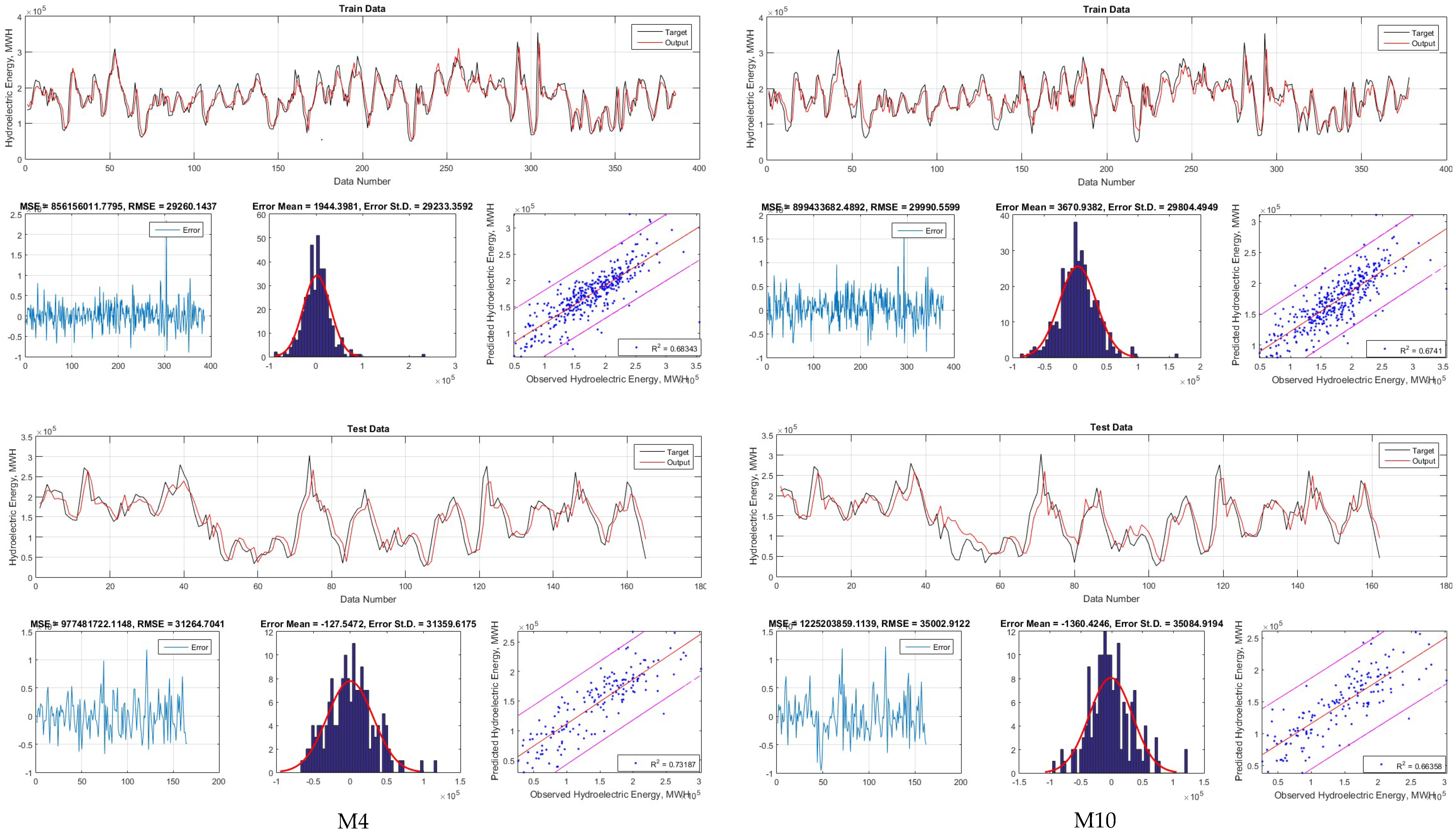
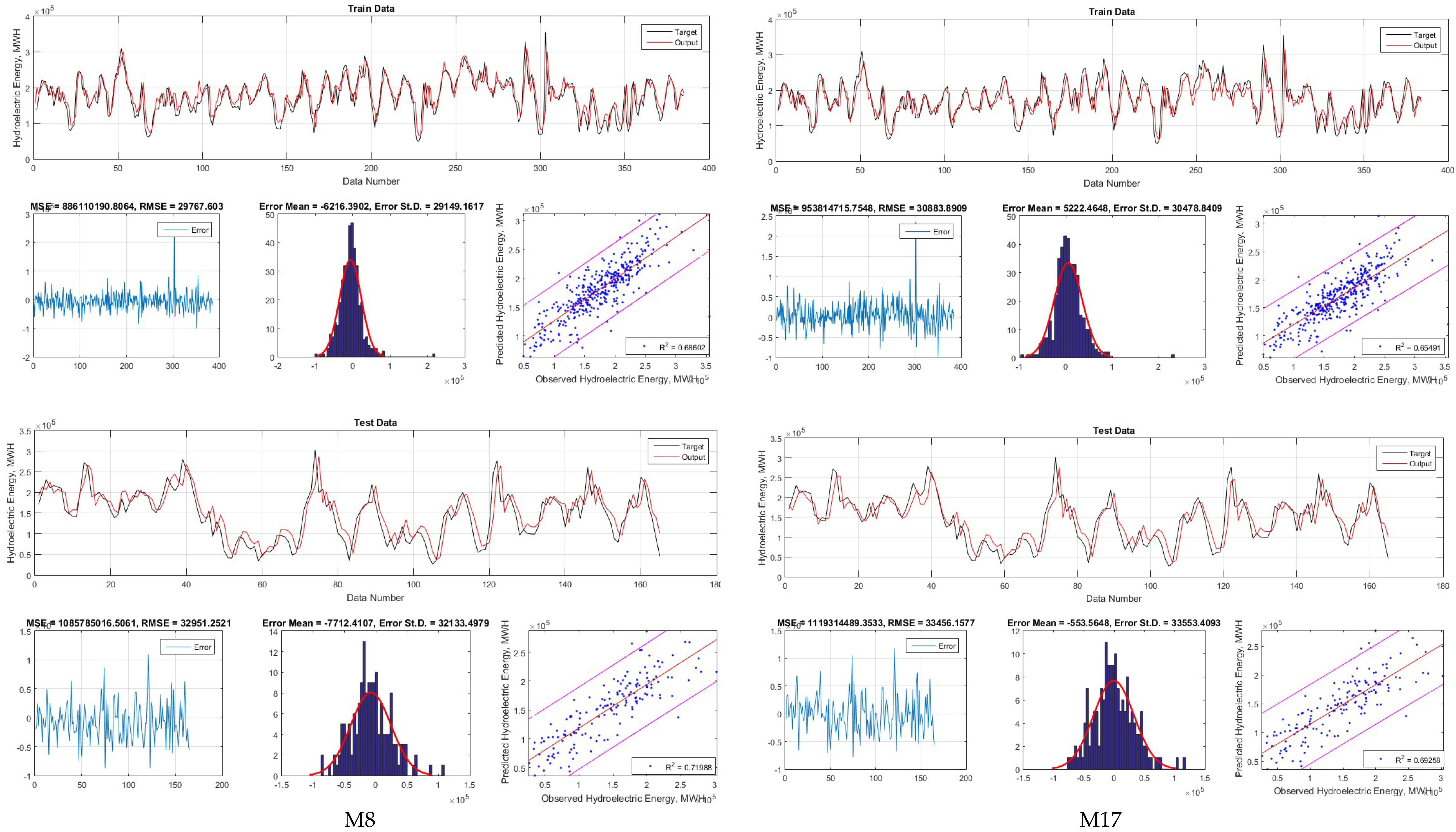
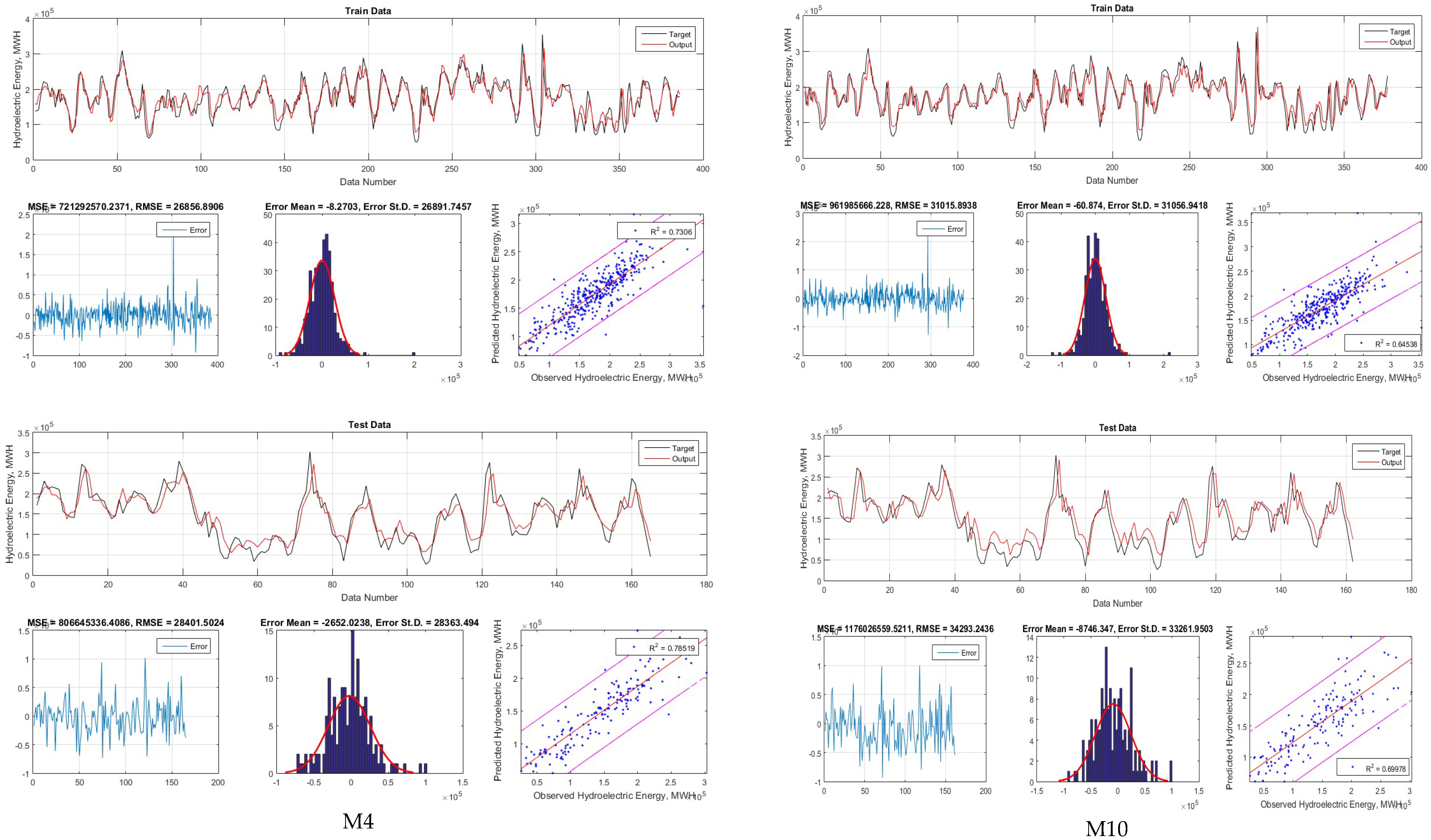
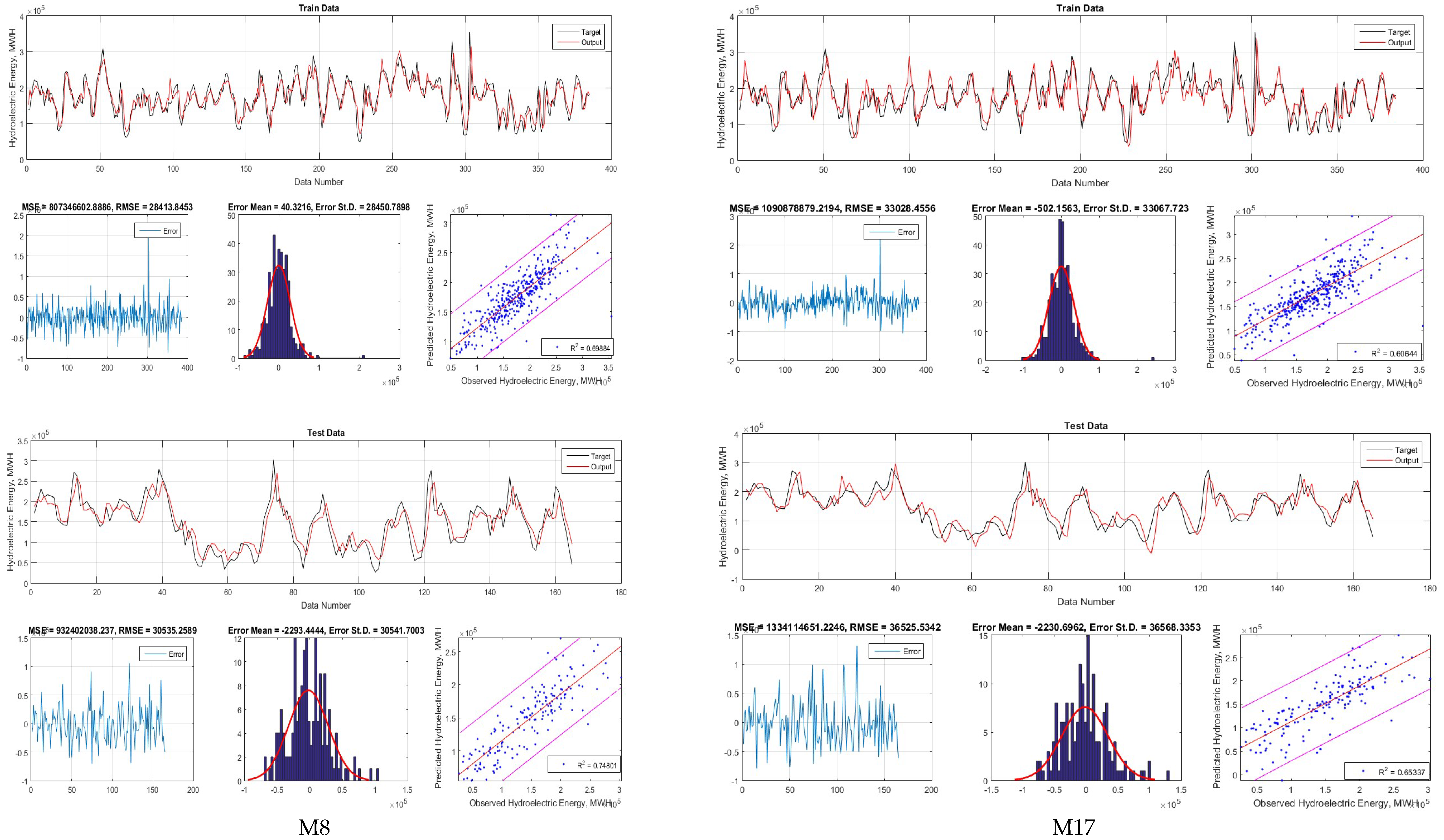
The assessment of the proposed model’s efficiencies, including accuracy and agreement, was evaluated using statistical criteria, such as the confidence index (CI), root mean square error (RMSE), Nash-Sutcliffe Efficiency (NSE), coefficient of determination (R²), index of agreement (d), relative absolute error (RAE) and mean absolute error (MAE).

The evaluation criteria of RMSE and MAE are common mean error indicators that indicated how close data points are to a best fit line (Equations (18) & (19)) [31].

According to Nash and Sutcliffe [32], the NSE is defined as the sum of the absolute squared differences of the observed and estimated data normalized by the variance minus one. (Equation (21)). As determined by [33], the range of NSE is from one to −∞. When NSE is less than 0, the mean observed value have been a better predictor than the model. It describes the plot of observed data versus estimated data, and how well they fit the 1:1 line.

Furthermore, according to Bravais-Pearson, the R² presents the squared value of the correlation coefficient describing how much of the observed dispersion is delivered by the prediction. The value of R² may vary from 1 and 0. The 0, and 1 values would present no correlation between observed and predicted data, and dispersion of the estimation data is equal to that of the observation, respectively [33] (Equation (20)).

The index of agreement d [34] prevail over the insensitivity of NSE and R² to differences in the means and variances of the observed and estimated data [35]. The index of agreement demonstrates the ratio of the mean square error and the potential error [36] (Equation (22)). The range of d similar to R² changes from 0 for the no correlation to 1, which is a perfect fit.

The RAE is a non-negative index that indicates a ratio of the overall agreement level between observed and estimated datasets. The range of RAE may change from 0 for a perfect fit to ∞, which means no upper bound. The Confidence index (CI) is the product of NSE and d, which ranges between 1 (perfect fit) and −∞. Lower than zero values means that the mean observed values have been a better predictor than the model.

The evaluation criteria were calculated based on the following equations:

$$RMSE=\sqrt{\frac{1}{N}}{\displaystyle \sum _{i=1}^N{\left(O_i-P_i\right)}^2},0\le RMSE<\infty$$

(18)

$$MAE=\frac{1}{N}{\displaystyle \sum _{i=1}^N\left|O_i-P_i\right|},0\le MAE<\infty$$

(19)

$$R^2={\left(\frac{{\displaystyle {\sum }_{i=1}^N\left(O_i-\overline{O}\right)\left(P_i-\overline{P}\right)}}{\sqrt{{\displaystyle {\sum }_{i=1}^N{\left(O_i-\overline{O}\right)}^2\sqrt{{\displaystyle {\sum }_{i=1}^N{\left(P_i-\overline{P}\right)}^2}}}}}\right)}^2,0\le r^2\le 1$$

(20)

$$NSE=1-\frac{{\displaystyle {\sum }_{i=1}^N{\left(O_i-P_i\right)}^2}}{{\displaystyle {\sum }_{i=1}^N{\left(O_i-\overline{O}\right)}^2}},-\infty <NSE\le 1$$

(21)

$$d=1-\frac{{\displaystyle {\sum }_{i=1}^N{\left(P_i-O_i\right)}^2}}{{\displaystyle {\sum }_{i=1}^N{\left(\left|P_i-\overline{O}\right|+\left|O_i-\overline{O}\right|\right)}^2}},0\le d\le 1$$

(22)

$$PI=1-\frac{{\displaystyle {\sum }_{i=1}^N{\left(O_i-P_i\right)}^2}}{{\displaystyle {\sum }_{i=1}^N{\left(O_i-O_{i-1}\right)}^2}},-\infty <PI<\infty$$

(23)

$$CI=d\times NSE,-\infty \le CI\le 1$$

(24)

$$RAE=\frac{{\displaystyle {\sum }_{i=1}^N\left|O_i-P_i\right|}}{{\displaystyle {\sum }_{i=1}^N\left|O_i-\overline{O}\right|}}$$

(25)

In which the O_i is observation value, P_i is the predicted model output, Ō is the average of observations, $\overline{P}$ is the average of model outputs and N is number of data.

3. Results

In this study, the inflow of the Dez dam and the average precipitation over the whole basin were utilized to forecast the hydropower generation. For this purpose, the time series divided into two subsets as the train and test subsets. 70% of data was assigned as the train and the remaining 30% for test phase.

Different input combinations were evaluated and used in the modeling process. The final selection of input combinations was based on the correlation analysis of variables in Table 3, the physical nature of variables and applicability of models presented in

Table 2. Different input combination used for ANFIS and GWO-ANFIS modeling.

Model	Input Parameters	Output
M1	Qt	Ht
M2	Qt, Pt	Ht
M3	Qt-1, Qt	Ht
M4	Qt-1, Qt, Ht-1	Ht
M5	Ht-1	Ht
M6	Qt-1, Qt, Pt, Ht-1	Ht
M7	Ht-2, Ht-1	Ht
M8	Qt, Ht-2, Ht-1	Ht
M9	Qt-1, Qt, Ht-2, Ht-1	Ht
M10	Ht-12, Ht-2, Ht-1	Ht
M11	Ht-12, Ht-1	Ht
M12	Ht-12	Ht
M13	Qt-4, Qt-3, Qt-2, Qt-1, Qt	Ht
M14	Qt-3, Qt-2, Qt-1, Qt	Ht
M15	Qt-2, Qt-1, Qt	Ht
M16	Qt-3, Qt-2, Ht-12, Ht-1	Ht
M17	Qt-3, Ht-2, Ht-1	Ht
M18	Qt-4, Qt-3	Ht
M19	Pt-5, Pt-4, Qt-4, Qt-3, Qt-2	Ht
M20	Pt-5, Pt-4, Qt-3, Qt-2	Ht

. Based on the availability of different measured parameters in the dam, one can choose which model is applicable for prediction of hydropower, and these different combinations strengthen the applicability of model in different data availability of the study. Some models were only based on inflow to the dam and rainfall such as: M1, M2, M3, M13, M14, M15, M18, M19 and M20. These models did not require the hydropower generation of the dam in previous time steps and, based on inflow and precipitation, can predict the hydropower generation in the plan. Some models used lagged values of hydropower generation of the dam in previous time steps as input vectors and these models did not require further information of inflow or precipitation in prediction of hydropower generation. These models, such as M5, M7 M10, M11 and M12, are lagged based models. The other models are based on combination of lagged values of hydropower generation, inflow and precipitation, such as M4, M6, M8, M9, M16 and M17.

According to Table 2, the discharge, precipitation, and the hydropower generation with different lags were used to forecast the hydropower generation for the next month. The correlation coefficients between the input variables were calculated and are presented in

Table 3. Correlation coefficients between parameters.

	Ht	Qt	Pt	Ht-1	Ht-2	Ht-3	Ht-4	Ht-5	Ht-6	Ht-12	Qt-1	Qt-2	Qt-3	Qt-4	Qt-5	Qt-6	Pt-1	Pt-2	Pt-3	Pt-4	Pt-5
Ht	1
Qt	0.11	1
Pt	0.05	0.13	1
Ht-1	0.66	0.01	0.1	1
Ht-2	0.34	0	0.07	0.66	1
Ht-3	0.15	0.02	0.02	0.34	0.66	1
Ht-4	0.06	0.02	0	0.16	0.35	0.66	1
Ht-5	0.02	0.01	0.02	0.06	0.16	0.35	0.67	1
Ht-6	0.01	0	0.08	0.02	0.06	0.16	0.35	0.66	1
Ht-12	0.18	0.01	0.06	0.14	0.08	0.04	0.02	0.01	0.01	1
Qt-1	0.27	0.46	0	0.11	0.01	0	0.02	0.02	0.01	0.09	1
Qt-2	0.31	0.14	0.09	0.27	0.11	0.01	0	0.02	0.02	0.15	0.46	1
Qt-3	0.31	0	0.19	0.31	0.26	0.11	0.01	0	0.02	0.17	0.14	0.46	1
Qt-4	0.24	0.02	0.24	0.31	0.31	0.26	0.11	0.01	0	0.13	0	0.14	0.46	1
Qt-5	0.11	0.11	0.18	0.24	0.31	0.31	0.26	0.11	0.01	0.05	0.03	0	0.14	0.46	1
Qt-6	0.02	0.17	0.04	0.11	0.24	0.31	0.31	0.26	0.11	0	0.11	0.03	0	0.14	0.46	1
Pt-1	0	0.45	0.23	0.06	0.1	0.07	0.02	0	0.02	0.01	0.13	0	0.09	0.19	0.24	0.18	1
Pt-2	0.04	0.39	0.06	0	0.06	0.1	0.07	0.02	0	0	0.45	0.13	0	0.09	0.19	0.24	0.23	1
Pt-3	0.11	0.29	0	0.04	0	0.06	0.1	0.07	0.02	0.03	0.39	0.45	0.13	0	0.09	0.19	0.06	0.23	1
Pt-4	0.2	0.14	0.06	0.1	0.04	0	0.06	0.1	0.07	0.08	0.28	0.39	0.45	0.13	0	0.09	0	0.06	0.23	1
Pt-5	0.21	0.02	0.2	0.2	0.1	0.04	0	0.06	0.1	0.12	0.14	0.28	0.39	0.45	0.13	0	0.06	0	0.06	0.23	1

; they oscillate between 0.01 and 0.67. It should be noted that Q is the inflow of the dam, but not the inflow of the turbine. Therefore, as the Dam is multipurpose, and the water stored in the dam is also used for irrigation, it is possible to use Q_t to predict the H_t. All 20 input combinations were used for modeling by ANFIS and GWO-ANFIS to evaluate the capability of GWO in optimizing the ANFIS parameters, which shows better performance. The results of ANFIS modeling are presented in

Table 4. Results of ANFIS modeling in train and test phases.

Train		ANFIS1	ANFIS2	ANFIS3	ANFIS4	ANFIS5	ANFIS6	ANFIS7	ANFIS8	ANFIS9	ANFIS10
	RSQ	0.08	0.12	0.17	0.68	0.62	0.51	0.63	0.69	0.66	0.67
	RMSE	179,477	179,882	179,305	29,260	32,165	38,263	31,488	29,768	30,164	29,991
	MAE	171,981	172,397	171,840	21,000	23,451	28,172	22,869	21,539	21,599	22,521
	RAE	4.10	4.11	4.11	0.50	0.56	0.67	0.55	0.51	0.52	0.54
	d	0.31	0.31	0.31	0.90	0.88	0.83	0.88	0.90	0.89	0.89
	NSE	−11.02	−11.08	−11.01	0.68	0.61	0.45	0.63	0.67	0.66	0.67
	CI	−3.41	−3.42	−3.41	0.61	0.54	0.38	0.56	0.60	0.59	0.60
		ANFIS11	ANFIS12	ANFIS13	ANFIS14	ANFIS15	ANFIS16	ANFIS17	ANFIS18	ANFIS19	ANFIS20
	RSQ	0.66	0.12	0.22	0.26	0.23	0.64	0.65	0.35	0.22	0.32
	RMSE	30,579	51,150	179,856	179,647	179,438	31,253	30,884	179,512	180,465	180,470
	MAE	23,091	40,660	172,323	172,134	171,954	22,451	22,071	172,115	172,932	172,973
	RAE	0.55	0.97	4.12	4.11	4.11	0.54	0.53	4.12	4.13	4.13
	d	0.89	0.54	0.31	0.31	0.31	0.88	0.89	0.31	0.31	0.31
	NSE	0.66	0.04	−11.06	−11.02	−11.01	0.64	0.64	−11.02	−11.11	−11.11
	CI	0.58	0.02	−3.41	−3.41	−3.41	0.56	0.57	−3.41	−3.43	−3.43
Test		ANFIS1	ANFIS2	ANFIS3	ANFIS4	ANFIS5	ANFIS6	ANFIS7	ANFIS8	ANFIS9	ANFIS10
	RSQ	0.12	0.15	0.21	0.73	0.70	0.64	0.67	0.72	0.69	0.66
	RMSE	155,453	155,740	155,021	31,265	33,984	36,654	35,367	32,951	33,508	35,003
	MAE	143,490	143,773	143,018	24,498	26,694	28,267	28,096	25,989	25,890	26,600
	RAE	2.85	2.85	2.83	0.49	0.53	0.56	0.56	0.51	0.51	0.53
	d	0.38	0.37	0.38	0.92	0.91	0.89	0.89	0.91	0.90	0.89
	NSE	−5.67	−5.69	−5.60	0.73	0.68	0.63	0.66	0.70	0.69	0.66
	CI	−2.13	−2.13	−2.11	0.67	0.62	0.56	0.59	0.64	0.62	0.59
		ANFIS11	ANFIS12	ANFIS13	ANFIS14	ANFIS15	ANFIS16	ANFIS17	ANFIS18	ANFIS19	ANFIS20
	RSQ	0.68	0.15	0.51	0.42	0.31	0.68	0.69	0.45	0.39	0.37
	RMSE	34,307	59,395	154,896	154,929	154,933	34,157	33,456	154,793	155,475	155,535
	MAE	25,910	45,123	142,788	142,914	142,926	26,613	25,956	142,809	143,361	143,448
	RAE	0.51	0.89	2.82	2.83	2.83	0.53	0.51	2.82	2.83	2.83
	d	0.90	0.64	0.38	0.38	0.38	0.90	0.90	0.38	0.38	0.38
	NSE	0.68	0.03	−5.56	−5.60	−5.60	0.68	0.69	−5.55	−5.61	−5.61
	CI	0.61	0.02	−2.10	−2.11	−2.11	0.61	0.62	−2.10	−2.11	−2.11

. Among the different input combinations, the first three models were not capable to reproduce satisfying results. Negative values were assigned to the NSE and CI, which show the poor application of models. The same procedure is visible in M13, M14, M15, M18, M19 and M20. However, the M4 to M11, M16 and M17 performed well. Among these combinations, M4 is the best and M8, M10 and M9 are the next in row. It should be noted that although the M4 was the best based on the evaluation criteria, according to Table 2, M17 was selected as the best model. This was because all the inputs of M17, i.e., Qt-3, Ht-2 and Ht-1, have at least a one-month lag. In addition, the results of M4 and M17 were not considerably different. This pattern was repeated for the test phase. Consequently, it can be concluded that, ANFIS was capable to forecast the hydropower generation satisfactorily.

In the next step, the coupled model of GWO-ANFIS was utilized for hydropower generation forecasting. Results are presented in

Table 5. Results of GWO-ANFIS modeling in train and test phases. G-A is the abbreviation of GWO-ANFIS.

Train		G-A1	G-A2	G-A3	G-A4	G-A5	G-A6	G-A7	G-A8	G-A9	G-A10
	RSQ	0.09	0.31	0.28	0.73	0.63	0.63	0.65	0.70	0.72	0.65
	RMSE	49,503	42,889	43,809	26,857	31,477	32,559	30,770	28,414	27,482	31,016
	MAE	40,463	33,764	35,873	19,773	22,984	25,600	22,453	20,854	20,365	22,675
	RAE	0.97	0.81	0.86	0.47	0.55	0.61	0.54	0.50	0.49	0.54
	d	0.39	0.68	0.66	0.92	0.88	0.84	0.88	0.91	0.91	0.88
	NSE	0.09	0.31	0.28	0.73	0.63	0.60	0.65	0.70	0.72	0.65
	CI	0.03	0.21	0.19	0.67	0.55	0.51	0.57	0.63	0.65	0.57
		G-A11	G-A12	G-A13	G-A14	G-A15	G-A16	G-A17	G-A18	G-A19	G-A20
	RSQ	0.64	0.18	0.48	0.42	0.33	0.68	0.61	0.32	0.41	0.37
	RMSE	31,073	47,263	37,224	39,510	42,411	29,521	33,028	42,668	39,952	41,037
	MAE	23,219	37,781	29,617	30,810	33,846	21,076	23,585	32,684	30,033	31,964
	RAE	0.55	0.90	0.71	0.74	0.81	0.50	0.56	0.78	0.72	0.76
	d	0.88	0.53	0.80	0.75	0.68	0.90	0.88	0.68	0.75	0.73
	NSE	0.64	0.18	0.48	0.42	0.33	0.68	0.59	0.32	0.41	0.37
	CI	0.57	0.09	0.39	0.32	0.22	0.61	0.52	0.22	0.30	0.27
Test		G-A1	G-A2	G-A3	G-A4	G-A5	G-A6	G-A7	G-A8	G-A9	G-A10
	RSQ	0.11	0.21	0.26	0.79	0.69	0.71	0.70	0.75	0.76	0.70
	RMSE	62,420	58,695	56,473	28,402	34,128	40,849	34,151	30,535	29,928	34,293
	MAE	50,699	45,595	46,289	21,439	27,079	32,838	27,480	24,131	23,811	27,566
	RAE	1.01	0.90	0.92	0.42	0.54	0.65	0.54	0.48	0.47	0.55
	d	0.44	0.58	0.54	0.93	0.89	0.79	0.89	0.92	0.92	0.89
	NSE	−0.07	0.05	0.12	0.78	0.68	0.54	0.68	0.74	0.75	0.68
	CI	−0.03	0.03	0.07	0.72	0.61	0.43	0.61	0.68	0.69	0.60
		G-A11	G-A12	G-A13	G-A14	G-A15	G-A16	G-A17	G-A18	G-A19	G-A20
	RSQ	0.69	0.13	0.51	0.48	0.35	0.73	0.65	0.35	0.45	0.43
	RMSE	33,816	59,590	47,204	49,583	54,710	31,377	36,526	54,756	48,849	52,456
	MAE	26,205	46,902	37,185	38,988	43,489	24,547	28,006	42,243	37,949	41,320
	RAE	0.52	0.93	0.73	0.77	0.86	0.49	0.55	0.83	0.75	0.82
	d	0.90	0.51	0.68	0.64	0.56	0.92	0.89	0.55	0.68	0.61
	NSE	0.69	0.02	0.39	0.32	0.18	0.73	0.63	0.18	0.35	0.25
	CI	0.61	0.01	0.27	0.21	0.10	0.67	0.57	0.10	0.24	0.15

. According to Table 5, the model performed well in all input combinations. As the d, NSE and CI values were positive in all the models, the new modeling technique of GWO-ANFIS provided a superior capability in forecasting hydropower generation, while the ANFIS results failed in nine models. In addition, based on the evaluation criteria, the accuracy of forecasting was higher for GWO-ANFIS.

The time series of observed and forecasted hydropower in train and test phases for M4, M8, M10 and M117 are presented in Figure 6 and Figure 7. Both ANFIS and GWO-ANFIS performed well, while the GWO-ANFIS was superior due to less error. In addition, it can be observed that the M4 and M10 presented better input combinations, while for dam operation and reservoir management, M17 was more practical.

Although Figure 6 and Figure 7 and Table 4 and Table 5 show the observed and forecasted values and evaluation criteria for all models, the error distribution among models could not be discussed via these figures and tables. Therefore, the box plot of error during the train and test phases was plotted in Figure 8. In Figure 8, it can be observed that the GWO-ANFIS was superior to the ANFIS considerably in almost all input combinations. Nevertheless, the error of ANFIS in nine models was considerably higher than the GWO-ANFIS.

The meta-heuristic optimization algorithm of GWO-ANFIS showed an acceptable efficiency in the optimization of the unknown parameters in ANFIS. Although the number of optimization parameters in ANFIS and GWO-ANFIS was the same, the main complexity quantifier was the number of unknown parameters to be tuned for model training. The present research sought to ensure that the numerical complexity of the two modeling approaches was similar. Furthermore, the ANFIS models required the derivative calculation for unknown parameters, which increased the computational time and space necessary for training. While the GWO-ANFIS models did not need the derivative calculation, this would lead to less computation and faster convergence.

4. Conclusions

In this study, a coupled of adaptive neuro-fuzzy inference system and grey wolf optimization was utilized for one month ahead hydropower generation. For this purpose, 53 years of monthly data of inflow to the dam reservoir and the hydropower generation were used. Twenty input-output combinations were considered to evaluate the model robustness and to find the best input-output combination. Based on the results, GWO was capable to improve the ANFIS performance considerably. GWO-ANFIS performed well in all 20 combinations based on the evaluation criteria while the ANFIS failed in nine out of 20 combinations. Additionally, the box plot of error in all combinations shows the superiority of GWO-ANFIS. Overall, it can be concluded that, GWO-ANFIS is capable to forecast the hydropower generation satisfactorily, which makes it a suitable tool for policymakers. Furthermore, for the future research direction, it is important to mention that, not all the rules in the model architecture are essential; thus, it is necessary to reduce trained models complexity through eliminating the noncontributing rules which leads to the reduction of network’s computational cost. To improve the proposed method, utilizing the other optimization algorithms for creating novel hybrid prediction models, as well as applying ensemble models in this application is suggested for the future research. In fact, the potential of ensemble machine learning models have not yet been fully explored in the prediction of hydropower generation, which leaves great room for future investigations. In addition, a limitation of our proposed model was that while the effective factors for which the model was implemented were the most critical factors, there may be other relevant factors that should be used. For instance, climate change and drought variations need to be separated from the general trend of the data set. Therefore, the addition of these concepts is left for future work.

References

1. Hamlet, A.F.; Huppert, D.; Lettenmaier, D.P. Economic value of long-lead streamflow forecasts for Columbia River hydropower. J. Water Resour. Plan. Manag. 2002, 1282, 91–101. [Google Scholar] [CrossRef]
2. Tang, G.L.; Zhou, H.C.; Li, N.; Wang, F.; Wang, Y.; Jian, D. Value of medium-range precipitation forecasts in inflow prediction and hydropower optimization. Water Resour. Manag. 2010, 24, 2721–2742. [Google Scholar] [CrossRef]
3. Zhou, H.; Tang, G.; Li, N.; Wang, F.; Wang, Y.; Jian, D. Evaluation of precipitation forecasts from NOAA global forecast system in hydropower operation. J. Hydroinform. 2011, 13, 81–95. [Google Scholar] [CrossRef]
4. Block, P. Tailoring seasonal climate forecasts for hydropower operations. Hydrol. Earth Syst. Sci. 2011, 15, 1355–1368. [Google Scholar] [CrossRef] [Green Version]
5. Rheinheimer, D.E.; Bales, R.C.; Oroza, C.A.; Lund, J.R.; Viers, J.H. Valuing year-to-go hydrologic forecast improvements for a peaking hydropower system in the Sierra Nevada. Water Resour. Res. 2016, 52, 3815–3828. [Google Scholar] [CrossRef] [Green Version]
6. Zhang, X.; Peng, Y.; Xu, W.; Wang, B. An Optimal Operation Model for Hydropower Stations Considering Inflow Forecasts with Different Lead-Times. Water Resour. Manag. 2017. [Google Scholar] [CrossRef]
7. Peng, Y.; Xu, W.; Liu, B. Considering precipitation forecasts for real-time decision-making in hydropower operations. Int. J. Water Resour. Dev. 2017, 33, 987–1002. [Google Scholar] [CrossRef]
8. Jiang, Z.; Li, R.; Li, A.; Ji, C. Runoff forecast uncertainty considered load adjustment model of cascade hydropower stations and its application. Energy 2018, 158, 693–708. [Google Scholar] [CrossRef]
9. Mosavi, A.; Ozturk, P.; Chau, K.W. Flood prediction using machine learning models: Literature review. Water 2018, 10, 1536. [Google Scholar] [CrossRef]
10. Hammid, A.T.; Sulaiman, M.H.B.; Abdalla, A.N. Prediction of small hydropower plant power production in Himreen Lake dam (HLD) using artificial neural network. Alexandria Eng. J. 2018, 57, 211–221. [Google Scholar] [CrossRef]
11. Boucher, M.A.; Ramos, M.H. Ensemble Streamflow Forecasts for Hydropower Systems. Handb. Hydrometeorol. Ensemble Forecast. 2018, 1–19. [Google Scholar] [CrossRef]
12. Choubin, B.; Moradi, E.; Golshan, M.; Adamowski, J.; Sajedi-Hosseini, F.; Mosavi, A. An Ensemble prediction of flood susceptibility using multivariate discriminant analysis, classification and regression trees, and support vector machines. Sci. Total Environ. 2019, 651, 2087–2096. [Google Scholar] [CrossRef] [PubMed]
13. Shamshirband, S.; Jafari Nodoushan, E.; Adolf, J.E.; Abdul Manaf, A.; Mosavi, A.; Chau, K.W. Ensemble models with uncertainty analysis for multi-day ahead forecasting of chlorophyll a concentration in coastal waters. Eng. Appl. Comput. Fluid Mech. 2019, 13, 91–101. [Google Scholar] [CrossRef]
14. Bui, K.T.T.; Bui, D.T.; Zou, J.; Van Doan, C.; Revhaug, I. A novel hybrid artificial intelligent approach based on neural fuzzy inference model and particle swarm optimization for horizontal displacement modeling of hydropower dam. Neural Comput. Appl. 2018, 29, 1495–1506. [Google Scholar]
15. Kim, Y.O.; Eum, H.I.; Lee, E.G.; Ko, I.H. Optimizing Operational Policies of a Korean Multireservoir System Using Sampling Stochastic Dynamic Programming with Ensemble Streamflow Prediction. J. Water Resour. Plan Manag. 2007, 133, 4. [Google Scholar] [CrossRef]
16. Ch, S.; Anand, N.; Panigrahi, B.K. Streamflow forecasting by SVM with quantum behaved particle swarm optimization. Neurocomputing 2013, 101, 18–23. [Google Scholar] [CrossRef]
17. Cote, P.; Leconte, R. Comparison of Stochastic Optimization Algorithms for Hydropower Reservoir Operation with Ensemble Streamflow Prediction. J. Water Resour. Plan Manag. 2016, 142, 04015046. [Google Scholar] [CrossRef]
18. Keshtegar, B.; Falah Allawi, M.; Afan, H.A.; El-Shafie, A. Optimized River Stream-Flow Forecasting Model Utilizing High-Order Response Surface Method. Water Resour. Manag. 2016, 30, 3899–3914. [Google Scholar] [CrossRef]
19. Paul, M.; Negahban-Azar, M. Sensitivity and uncertainty analysis for streamflow prediction using multiple optimization algorithms and objective functions: San Joaquin Watershed, California. Model. Earth Syst. Environ. 2018, 4, 1509–1525. [Google Scholar] [CrossRef]
20. Karballaeezadeh, N.; Mohammadzadeh, D.; Shamshirband, S.; Hajikhodaverdikhan, P.; Mosavi, A.; Chau, K.W. Prediction of remaining service life of pavement using an optimized support vector machine. Eng. Appl. Comput. Fluid Mech. 2019, 16, 120–144. [Google Scholar]
21. Niu, M.; Wang, Y.; Sun, S.; Li, Y. A novel hybrid decomposition-and-ensemble model based on CEEMD and GWO for short-term PM2.5 concentration forecasting. Atmos. Environ. 2016, 134, 168–180. [Google Scholar] [CrossRef]
22. Jang, J.-S.R. ANFIS: Adaptive-network-based fuzzy inference system. IEEE Trans. Syst. Man Cybern. 1993, 23, 665–685. [Google Scholar] [CrossRef]
23. Choubin, B.; Khalighi-Sigaroodi, S.; Malekian, A.; Kişi, O. Multiple linear regression, multi-layer perceptron network and adaptive neuro-fuzzy inference system for the prediction of precipitation based on large-scale climate signals. Hydrol. Sci. J. 2016, 61, 1001–1009. [Google Scholar] [CrossRef]
24. Firat, M.; Güngör, M. Hydrological time-series modelling using an adaptive neuro-fuzzy inference system. Hydrol. Process. 2007, 22, 2122–2132. [Google Scholar] [CrossRef]
25. Shabri, A. A Hybrid Wavelet Analysis and Adaptive Neuro-Fuzzy Inference System for Drought Forecasting. Appl. Math. Sci. 2014, 8, 6909–6918. [Google Scholar] [CrossRef]
26. Kisi, O.; Shiri, J. Precipitation forecasting using wavelet genetic programming and wavelet-neuro-fuzzy conjunction models. Water Resour. Manag. 2011, 25, 3135–3152. [Google Scholar] [CrossRef]
27. Awan, J.A.; Bae, D.H. Drought prediction over the East Asian monsoon region using the adaptive neuro-fuzzy inference system and the global sea surface temperature anomalies. Int. J. Climatol. 2016, 36, 4767–4777. [Google Scholar] [CrossRef]
28. Mirjalili, S.; Mirjalili, S.M.; Lewis, A. Grey wolf optimizer. Adv. Eng. Softw. 2014, 69, 46–61. [Google Scholar] [CrossRef]
29. Bozorg-Haddad, O. Advanced Optimization by Nature-Inspired Algorithms; Springer: Singapore, 2017. [Google Scholar]
30. Muro, C.; Escobedo, R.; Spector, L.; Coppinger, R. Wolf-pack (Canis Lupus) hunting strategies emerge from simple rules in computational simulations. Behav. Process. 2011, 88, 192–197. [Google Scholar] [CrossRef]
31. Amr, H.; El-Shafie, A.; El Mazoghi, H.; Shehata, A.; Taha, M.R. Artificial neural network technique for rainfall forecasting applied to Alexandria, Egypt. Int. J. Phys. Sci. 2011, 6, 1306–1316. [Google Scholar]
32. Nash, J.E.; Sutcliffe, J.V. River flow forecasting through conceptual models part I—A discussion of principles. J. Hydrol. 1970, 10, 282–290. [Google Scholar] [CrossRef]
33. Krause, P.; Boyle, D.P.; Bäse, F. Comparison of different efficiency criteria for hydrological model assessment. Adv. Geosci. 2005, 5, 89–97. [Google Scholar] [CrossRef] [Green Version]
34. Willmott, C.J. On the validation of models. Phys. Geogr. 1981, 2, 184–194. [Google Scholar] [CrossRef]
35. Legates, D.R.; McCabe, G.J. Evaluating the use of “goodness-of-fit” measures in hydrologic and hydroclimatic model validation. Water Resour. Res. 1999, 35, 233–241. [Google Scholar] [CrossRef]
36. Willmott, C.J. On the evaluation of model performance in physical geography. In Spatial Statistics and Models; Springer: Dordrecht, The Netherlands, 1984; pp. 443–460. [Google Scholar]
Figure 1. Location of the Dez dam and the precipitation stations in Iran.
Energies 12 00289 g001
Figure 2. Average monthly precipitation in the catchment and mean monthly inflow to the Dez dam reservoir.
Energies 12 00289 g002
Figure 3. Average power generation in the Dez hydropower plant.
Energies 12 00289 g003
Figure 4. Architecture of adaptive neuro-fuzzy inference system in this study.
Energies 12 00289 g004
Figure 5. The flowchart of ANFIS-GWO modeling.
Energies 12 00289 g005
Figure 6. Observed and forecasted time series of hydropower generation using ANFIS.
Energies 12 00289 g006aEnergies 12 00289 g006b
Figure 7. Observed and forecasted time series of hydropower generation using GWO-ANFIS.
Energies 12 00289 g007aEnergies 12 00289 g007b
Figure 8. Box plot of errors for ANFIS and GWO-ANFIS modeling in training and testing phases. F and G refer to ANFIS and GWO-ANFIS, respectively.
Energies 12 00289 g008