Research on Modeling and Hierarchical Scheduling of a Generalized Multi-Source Energy Storage System in an Integrated Energy Distribution System

Abstract

Energy storage systems play a crucial role in ensuring stable operation. However, the development of system-level energy storage is hindered due to the restrictions of economy, geography, and other factors. Transitions of traditional power systems into integrated energy distribution systems (IEDS) have provided new solutions to the problems mentioned above. Through intelligent control management methods, the utilization of multi-energy-type resources both on the supply and demand sides shows the potential for equivalent storage characteristics. Inspired by the aggregation principles, this paper aims at proposing a novel model named generalized multi-source energy storage (GMSES), including the modeling and cooperation of three kinds of available resources: conventional energy storage (CES), multi-energy flow resources (MFR), and demand response resources (DRR). Compared with the conventional means of storage, GMSES can be regarded as a more cost-effective and flexible participant in the proposed hierarchical energy scheduling framework that can realize system-level storage services in IEDS. On this basis, a multi-timescale energy scheduling strategy is proposed to reshape the regulation of IEDS operations and deal with the fluctuations caused by renewable energy and loads, where the general parameter serialization (GPS)-based control strategy is utilized to select and control the responsive loads in DRR. Furthermore, a hierarchical scheduling algorithm is developed to generate the optimal set-points of GMSES. Case studies are analyzed in an electricity-gas coupled IEDS. The simulation results show that the coupled co-optimization GMSES model is conducive to achieving the goal of self-management and economical operation, while the influence of the underlying IEDS on the upper energy system is reduced, as the tie-line power fluctuations are smoothed out.

1. Introduction

Energy storage systems (ESSs) play important roles in improving economy [1], energy supply stability [2], and energy efficiency [3]. Relative demonstrations around the world show that ESS is conducive to promoting efficient energy consumption and renewable energy integration. In the U.S., ESS is highly supported and widely applied in different power utility companies [4]. In Europe, ESS is regarded as one of the significant energy strategies in the Strategic Energy Technology (SET) Plan by the European Commission, which facilitates the European Union’s efforts to achieve energy targets by 2020 and 2050 [5].

Based on their operation mechanisms, ESSs can primarily be divided into electromagnetic, mechanical, electrochemical, and thermal ones, as shown in Figure 1 [6]. Previous studies have shown an urgent demand for system-level energy storage with low costs and high flexibility. However, owing to the restrictions of physical properties and commercial factors, the conventional energy storage model needs further improvement for the following reasons: (1) the energy storage economics are of significant concern, both in the investment stage and the operation stage [7]; (2) the application of ESS is limited by geography and external environment [8]; (3) durable system-level storage services could be affected by ESS capacity, cycle life, performance, and other factors [9]. Typical ESS storage characteristics, i.e., rated power, average capital cost, response time and applications, are classified in Figure 1 [6,7].

Some methods have been proposed to improve the existing energy storage model. In reference [10], due to the development and innovation on the physical materials of ESS, the energy efficiency of a vanadium redox flow battery was improved from 62% to 76%. A dispatching method for hybrid ESS was developed to minimize the life cycle cost in [11]. In reference [12], water heaters and battery storage systems were coordinated for optimum demand response, controlled by a proposed mathematical model. These studies were able to improve the performance and controllability of ESS to some extent. However, controllable resources of multi-energy networks, demand side and supply side, possess regulatable potential that hasn’t been coordinated efficiently in previous studies. Therefore, the energy storage model still faces challenges of high cost, limited power output, and lack of all-around applicability. Even though investment in energy storage is expected to decrease in the future, the median capital cost of a battery system for an 8-h battery, for example, is still predicted to be more than 1000 $/kW [13].

On the other hand, traditional power systems are undergoing transitions towards integrated energy distribution systems (IEDS) [14], where the interdependencies and synergy effects among various energy sectors are highlighted, including the electric power system (EPS), natural gas system (NGS), and district heating system (DHS). The transitions have gained popularity in both academia and industry [15]. In addition, controllable resources both on the supply and demand sides can be regulated and integrated as flexible participants [16,17], which also provides new pathways to the development of ESSs. In reference [18], home microgrids consisting of multiple distributed energy resources are taken as players in the market, whose power is well dispatched with the hierarchical bi-level controller. A bi-level model for long-term planning on wind investment is studied in [19], where demand- side resources and wind turbines are coordinated. Considering the link function between primary and secondary energy sources, electricity is taken as the core of IEDS. However, other types of energy carriers are necessary in the following analysis, as they can provide energy backup and enhance flexibility with respect to their complementary characteristics.

In this regard, this paper proposes a generalized multi-source energy storage (GMSES) model and its hierarchical optimal scheduling strategy for operation and control. Three kinds of controllable resources in GMSES are highlighted herein: conventional energy storage (CES), multi-energy flow resources (MFR), and demand response resources (DRR); and energy carriers such as electricity, gas, and heat are taken into consideration [20]. Interactions between electricity and other energy carriers are feasible due to energy conversion technologies. As electricity shows a core position in energy supply and unique characteristics in energy utilization, the GMSES power interaction mainly refers to electricity in this paper. Direct application of other energy carriers will be discussed in following papers.

The applications of advanced metering infrastructure (AMI) and information and communication technology (ICT) motivate the development of energy scheduling on multiple time scales. Owing to the uncertainties of the renewable energy and energy loads, there are power deviations between the forecast results and real-time operation status [21], which may influence the energy scheduling plan significantly. In this regard, day-ahead scheduling results need to be adjusted in response to the updated energy forecast information. GMSES resources can be adopted for power regulation to obtain stable operation. Therefore, three scheduling scenarios are addressed: day-head, intra-hour, and ultra-short-term.

However, response characteristics of GMSES resources vary in multi-time scales. In this case, a hierarchical framework may provide an appropriate way to solve this problem. A novel framework is presented in [22] to study the impacts of investment incentives on generation expansion planning. Based on a two-stage energy management strategy, wind power and plug-in electrical vehicles were able to be used to minimize its operational cost and maintain the power balance in [23]. In reference [24], with the hierarchical framework, the battery energy-storage system and renewable energy sources could be combined to realize an economic generation schedule. Inspired by this, a hierarchical scheduling framework for resource coordination is proposed for GMSES, where efficient energy interactions are feasible between the system-level instructions and equipment response. Accordingly, with the help of optimal scheduling planning and reasonable control strategies, integrated controllable resources of GMSES can realize the flexible energy flow utilization and meet the requirements of system-level storage service in IEDS.

The main contributions of this paper are summarized as follows.

(1)

By combining the resources of conventional energy storage, multi-energy flow and demand response, a novel model named GMSES is proposed for a system-level equivalent energy storage effect.

(2)

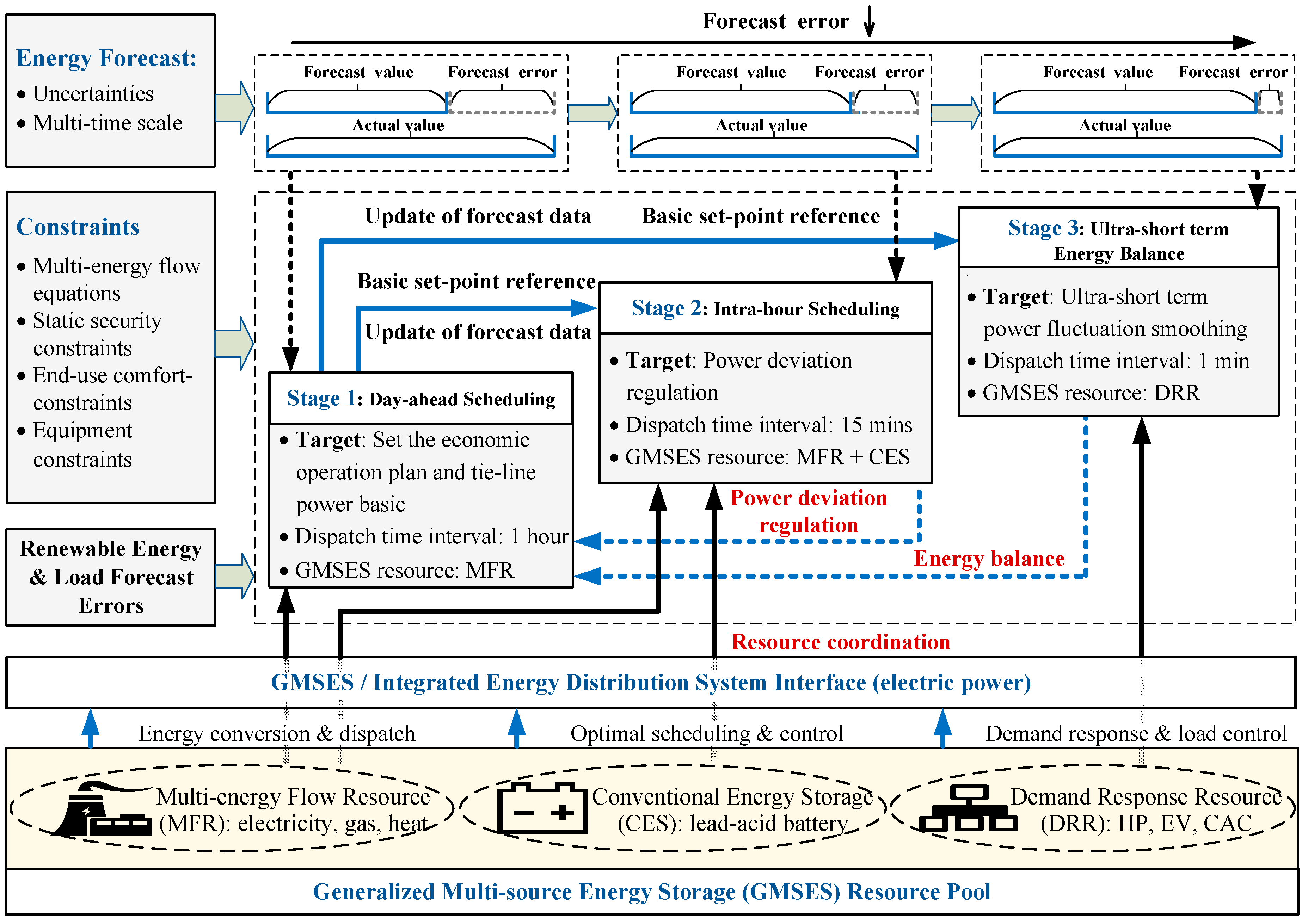
A hierarchical scheduling framework is studied to take advantage of complementary characteristics of various resources in GMSES and meet the precise response to the control target.

(3)

A coupled co-optimization model is developed for multi-type and multi-timescale coordinated scheduling solution (including day-ahead, intra-hour and ultra-short-term scheduling), promoting the economical and stable operation of IEDS.

(4)

A general parameter serialization (GPS)-based control strategy is adopted for the flexible demand-side loads in GMSES.

The rest of this paper is organized as follows: Section 2 describes a functional framework and the comprehensive modeling of GMSES. Section 3 presents a detailed description of the hierarchical scheduling framework, as well as the multi-timescale optimization and control strategy of GMSES. Verified by the case studies, Section 4 discusses the results for the economic scheduling and energy balance service of GMSES. Finally, Section 5 draws the conclusions.

2. Functional Framework and Comprehensive Modeling of Generalized Multi-Source Energy Storage

By coordinating the available resources of conventional energy storage, multi-energy flow and demand response, GMSES is characterized by its advantage of combining high power density and high energy density [25]. Complementary potential can be found in the coordination of GMSES controllable resources, as it varies in time scales and operation characteristics, as shown in Figure 1. This paper takes shorter scheduling scenarios of day-ahead, intra-hour and ultra-short-term as an example to illustrate the details of GMSES resources.

(1)

CES mainly refers to traditional battery energy storage in this paper. Currently, some typical CESs (i.e., lead-acid battery, lithium-ion battery, etc.) have been widely utilized for EPS applications [25]. To simplify the CES model, the lead-acid battery is selected with an operation time interval of 15 min to avoid too much power loss and lifecycle decrease caused by frequent dispatch [26].

(2)

MFR refers to the equivalent storage based on energy conversion and dispatch. Due to the microturbine response characteristics, MFR can be applied for longer time-scale dispatch schemes ranging from 15 min to 1 h in this paper, aiming at minimizing the operation costs in day-ahead scheduling and smoothing out the fluctuations in intra-hour scheduling [27].

(3)

DRR refers to the equivalent storage that aggregates flexible demand-side loads with reasonable control strategies [28]. Considering the fast-response characteristics of DRR, three typical controllable loads, i.e., heat pump (HP), central air conditioning (CAC), and electric vehicle (EV) are studied herein for energy balance service. The DRR operation time interval is set as 1 min.

As the application scenario and available resources may change, other energy storage resources like power-to-gas (P2G) [29] will be integrated in GMSES model in a subsequent study. Specifically, due to the larger energy storage potential, P2G can be deployed to adjust high-level renewable energy penetration [30]. Meanwhile, in this paper, considering the application scenario and energy scheduling timescale, P2G systems are not included in the GMSES model.

In Figure 2, the day-ahead schedule plan is studied in Stage 1 based on the optimal energy flow calculation, where the basic operation points of GMSES can be obtained. As the uncertainties vary in multiple time scales, the fluctuations caused by energy demand and renewable energy need to be smoothed out in the intra-hour schedule plan in Stage 2, and energy balance service is provided to follow the real-time variations in the ultra-short-term schedule plan in Stage 3, as shown in Figure 2. With flexible GMSES resources and the self-management energy scheduling strategy, the local impacts on the upper level energy system can be minimized.

2.1. GMSES-Conventional Energy Storage (CES)

The CES stores energy based on a series of energy storage cells. To evaluate the stored energy level, the state of charge (SOC) is studied as a significant indicator. It is modeled as shown in Equations (1)–(3), where the SOC time continuity characteristic can be found. The overcharging or overdischarging status is not allowed in the normal operation of GMSES-CES. Therefore, the SOC variations are limited to the operation constraints, as shown in Equations (4) and (5). In addition, it is assumed that the energy loss of the CES only occurs in the charging or discharging periods, and the SOC at the initial moment should be equal to that at the last moment in an operation period, as shown in Equation (6).

$$S_{\mathrm{SOC}\_k}(t)-S_{\mathrm{SOC}\_k}(t-\Delta t)=\Delta S_{\mathrm{SOC}\_k}(t)$$

(1)

$$\overline{\Delta S_{\mathrm{SOC}\_k}}=P_{k,\mathrm{C}}^{\mathrm{CES}}{\eta }_{k,\mathrm{C}}\Delta t/W_{k,\mathrm{rated}}^{\mathrm{CES}}$$

(2)

$$\underset{\_}{\Delta S_{\mathrm{SOC}\_k}}=P_{k,\mathrm{D}}^{\mathrm{CES}}\Delta t/(W_{k,\mathrm{rated}}^{\mathrm{CES}}{\eta }_{k,\mathrm{D}})$$

(3)

$$\underset{\_}{\Delta S_{\mathrm{SOC}\_k}}\le \Delta S_{\mathrm{SOC}\_k}(t)\le \overline{\Delta S_{\mathrm{SOC}\_k}}$$

(4)

$$\underset{\_}{S_{\mathrm{SOC}\_k}}\le S_{\mathrm{SOC}\_k}(t)\le \overline{S_{\mathrm{SOC}\_k}}$$

(5)

$$S_{\mathrm{SOC}\_k}(0)=S_{\mathrm{SOC}\_k}(\mathrm{T})$$

(6)

2.2. GMSES Multi-Energy Flow Resource (MFR)

Energy conversion and dispatch technologies have promoted flexible energy coupling and multi-energy complementary integration in IEDS. Taking electricity as an example, with the help of power electronic devices, bi-directional power flow can be realized if reasonable control strategy is implemented. That is to say, the energy-coupling links and multiple energy systems coupled thereto can be integrated and regulated as equivalent energy storage, which is defined as a multi-energy flow resource (MFR) in the framework of GMSES. Therefore, the regulatable potential of multi-energy networks could be fully utilized to support the EPS. An example of GMSES-MFR is shown in Figure 3.

The physical basis of GMSES-MFR is the bi-directional energy hub (BEH), and its charging status is defined as when electricity flows into the BEH, and the opposite defines the discharging status. Traditionally, the energy hub (EH) model has been widely used for multi-energy flow analysis. However, it is not able to explain bi-directional energy flow characteristics. Taking the EH type I in Figure 3b as an example, when the electricity generated by combined heat and power (CHP) satisfies the demand-side requirements, the excess parts can be sent back to the EPS, which makes P_e1 negative. At this time, the power flows into the air-conditioner (AC) system are negative, as the dispatch factor is non-negative. Obviously, this is unreasonable in reality. Hence, the BEH model is studied as below, where power electronic convertor (PEC) makes it possible for bi-directional power flow [31].

To describe the behaviors of energy dispatch in GMSES-MFR, ${\lambda }_{\mathrm{C}}$ and ${\lambda }_{\mathrm{D}}$ of BEH are defined as dispatch factors in the charging/standby and discharging status. Specifically, taking BEH type I as an example, when MFR is in the charging status, the load demand is satisfied by both EPS and NGS while $P_{\mathrm{e}1}$ is positive. If the ratio of $L_{\mathrm{h}1}$ to $L_{\mathrm{e}1}$ is equal to the heat-power ratio of CHP, the NGS can supply both electrical and thermal loads, which means that GMSES-MFR is in the standby status and $P_{\mathrm{e}1}$ is zero. When the gas input $P_{\mathrm{g}1}$ increases, the electricity generated by CHP could be sent back to the EPS through the PEC, which means that the MFR is discharging and $P_{\mathrm{e}1}$ is negative. BEH type I in charging/standby and discharging status can be modeled using Equations (7) and (8).

$$\left[\begin{array}{l}{L}_{\mathrm{e}1}\\ L_{\mathrm{h}1}\end{array}\right]=\left[\begin{array}{cc}1-{\lambda }_{\mathrm{C}1}& {\eta }_{\mathrm{CHP}}^{\mathrm{e}}\\ {\lambda }_{\mathrm{C}1}{\eta }^{\mathrm{AC}}& {\eta }_{\mathrm{CHP}}^{\mathrm{h}}\end{array}\right]\left[\begin{array}{l}{P}_{\mathrm{e}1}\\ P_{\mathrm{g}1}\end{array}\right]$$

(7)

$$\left[\begin{array}{l}{L}_{\mathrm{e}1}\\ L_{\mathrm{h}1}\end{array}\right]=\left[\begin{array}{cc}-1/(1-{\lambda }_{\mathrm{D}1})& {\eta }_{\mathrm{CHP}}^{\mathrm{e}}\\ -{\lambda }_{\mathrm{D}1}{\eta }^{\mathrm{AC}}/(1-{\lambda }_{\mathrm{D}1})& {\eta }_{\mathrm{CHP}}^{\mathrm{h}}\end{array}\right]\left[\begin{array}{l}{P}_{\mathrm{e}1}\\ P_{\mathrm{g}1}\end{array}\right]$$

(8)

Similarly, BEH type II in charging/standby and discharging status could be modeled in Equations (9) and (10).

$$\left[\begin{array}{l}{L}_{\mathrm{e}2}\\ L_{\mathrm{h}2}\end{array}\right]=\left[\begin{array}{cc}1& {\lambda }_{\mathrm{C}2}{\eta }_{\mathrm{CHP}}^{\mathrm{e}}\\ 0& (1-{\lambda }_{\mathrm{C}2}){\eta }^{\mathrm{GB}}+{\lambda }_{\mathrm{C}2}{\eta }_{\mathrm{CHP}}^{\mathrm{h}}\end{array}\right]\left[\begin{array}{l}{P}_{\mathrm{e}2}\\ P_{\mathrm{g}2}\end{array}\right]$$

(9)

$$\left[\begin{array}{l}{L}_{\mathrm{e}2}\\ L_{\mathrm{h}2}\end{array}\right]=\left[\begin{array}{cc}-1& {\lambda }_{\mathrm{D}2}{\eta }_{\mathrm{CHP}}^{\mathrm{e}}\\ 0& (1-{\lambda }_{\mathrm{D}2}){\eta }^{\mathrm{GB}}+{\lambda }_{\mathrm{D}2}{\eta }_{\mathrm{CHP}}^{\mathrm{h}}\end{array}\right]\left[\begin{array}{l}{P}_{\mathrm{e}2}\\ P_{\mathrm{g}2}\end{array}\right]$$

(10)

The energy conversion and dispatch processes can be obtained via energy coupling component. Therefore, the output power boundaries of the BEH can be illustrated as

$$\mathrm{Type}\mathrm{I}\{\begin{array}{l}{P}_{\mathrm{e}1}^{\mathrm{lb}}=L_{\mathrm{e}1}-P_{\mathrm{CHP}}^{\mathrm{e},\max }+k^{\mathrm{lb}}\\ P_{\mathrm{e}1}^{\mathrm{ub}}=L_{\mathrm{e}1}+P_{\mathrm{AC}}^{\mathrm{e},\max }/{\eta }^{\mathrm{AC}}+k^{\mathrm{ub}}\end{array}$$

(11)

$$\mathrm{Type}\mathrm{II}\{\begin{array}{l}{P}_{\mathrm{e}2}^{\mathrm{lb}}=L_{\mathrm{e}2}-P_{\mathrm{CHP}}^{\mathrm{e},\max }+k^{\mathrm{lb}}\\ P_{\mathrm{e}2}^{\mathrm{ub}}=L_{\mathrm{e}2}+k^{\mathrm{ub}}\end{array}$$

(12)

where k represents the correction factor of the effect of energy sectors on the output of P_e. It should be pointed out that the method of multi-energy flow analysis could also be applied to other scenarios in the IEDS.

The participation of NGS has broadened the border of energy regulation in GMSES, where energy flow analysis is adopted for the coupling relationship consideration. The mass-flow balance equation of NGS can be calculated in Equation (13). Furthermore, the interfaces between BEH and NGS mainly refer to the BEH consumed gas power P_g1 and P_g2, which influence the gas demand ${\omega }_{l,i}$ and ${\omega }_{l,j}$ at the connected node i and node j in Equation (14) and are constrained by the gas pressure level in Equation (15). As the IEDS discussed in this paper involves low-pressure scenarios, Lacey’s equation is used to express the relation between gas flow and pressure drop, as shown in Equation (16) [32]. The natural gas flow calculation could be solved using the Newton–Raphson method, the details for which can be found in [32].

$${\mathit{A}}_{\mathrm{NGS}}{\mathit{Q}}_r+{\mathit{\omega }}_s-{\mathit{\omega }}_l=\mathbf{0}$$

(13)

$$\left[\begin{array}{l}{\omega }_{l,i}^{\mathrm{with}}\\ {\omega }_{l,j}^{\mathrm{with}}\end{array}\right]=\left[\begin{array}{l}{\omega }_{l,i}^{\mathrm{without}}\\ {\omega }_{l,j}^{\mathrm{without}}\end{array}\right]+\left[\begin{array}{l}\frac{P_{g1}}{\mathrm{GHV}}\\ \frac{P_{g2}}{\mathrm{GHV}}\end{array}\right]$$

(14)

$$\Delta p_r=-0.5\times \frac{S_g{v}_g^2{f}_r{L}_r}{D_{\mathrm{p}}}$$

(15)

$$Q_r=5.72\times {10}^{-4}\sqrt{[\frac{(\Delta p_r)D_{\mathrm{p}}^5}{f_r{L}_r{S}_g}]}$$

(16)

2.3. GMSES Demand Response Resource (DRR)

When applied to ultra-short-term scheduling, the energy storage capacities required, as well as the investment costs and the power losses of GMSES-CES, will increase significantly, while the GMSES-MFR is not suitable for frequent adjustment due to the microturbines’ inherent response characteristics [33]. Therefore, to accommodate the forecast errors flexibly and economically, DRR with fast-response characteristics is utilized to manage the energy consumption of different load groups [33]. With the corresponding control strategy, DRR could be implemented to provide the required power increase or decrease, which is similar to the energy storage effect. The DRR considered herein primarily refers to the typical power-controllable flexible loads, including EV and temperature-controlled loads such as HP and CAC, which are widely used in the household, industry and commerce.

2.3.1. General Model of GMSES-DRR

The key operation parameters of DRRs have common characteristics such as being controllable, sequenceable, and combinable [12], and they can be expressed by general parameters to construct a general model of GMSES-DRR [34]. The operation characteristics with respect to key operation parameters and consumed power of DRRs are shown in Figure 4, where the power consumptions of HP and CAC have a corresponding thermoelectric coupling relationship with the location’s room temperature, as shown in Figure 4a,b, respectively. In contrast to the HP temperature curve, the charging state and energy status of EV determine its power consumption, as shown in Figure 4c.

In addition to the operation characteristics of different DRRs, the general model of controllable load groups could be further described by the dynamic mechanism and physical-power coupling model [28]. A typical DRR dynamic mechanism is proposed in Equation (17).

$${\mathit{E}}_{m_n}=(E_{m_n}^1,E_{m_n}^2,\dots ,E_{m_n}^h,\dots ,E_{m_n}^{\mathrm{H}})$$

(17)

Taking the operation status $E_{m_n}^h$ as an example, its dynamic mechanism can be described by Equation (18).

$$R{E}_{m_n,h}^{t+\Delta t}=f(T{P}_1,\dots ,T{P}_o,\dots ,T{P}_{\mathrm{O}},Q_1^t,\dots ,Q_a^t,\dots ,Q_{\mathrm{A}}^t,F_1^t,\dots ,F_b^t,\dots ,F_{\mathrm{B}}^t)$$

(18)

The operation power of DRR is determined by its own operation control variables and rated power, while the operation control variables are determined by the load’s key operation parameters and operation conditions in consecutive periods. In general, the operation power consumption of DRR has a certain correspondence with the key operation parameters. Taking DRR in operation status $E_{m_n}^h$ as an example, the physical-power coupling model formed by the key operation parameters can be illustrated by Equations (19) and (20).

$$P_{m_n}^h=r(F_{m_n}^h,P_{m_n,\mathrm{rated}}^h,{\eta }_{m_n}^h)$$

(19)

$$F_{m_n,h}^{t+\Delta t}=\{\begin{array}{cc}\mathrm{U}& Q_a^t\le Q_{a,-}^t\\ \mathrm{V}& Q_a^t\ge Q_{a,+}^t\\ F_{m_n,h}^t& else\end{array}$$

(20)

Based on the physical-power coupling model, the consumed power of DRR could be controlled and regulated by changing the physical parameters. The model parameters and coupling variables of the above three kinds of DRR are shown in

Table 1. Model parameters and coupling variables of DRRs.

Name	$\mathit{T}{\mathit{P}}_{\mathit{o}}$	${\mathit{Q}}_{\mathit{a}}^{\mathit{t}}$	${\mathit{F}}_{\mathit{b}}^{\mathit{t}}$	$\mathbf{U},\mathbf{V}$
HP	thermodynamic parameters of related buildings	indoor temperature	on/off state	close-0 open-1
EV	energy state	energy state energy state boundaries	charging state	idle-0 charge-1
CAC	thermodynamic parameters of related buildings	indoor temperature	load rate	heating mode non-heating mode

.

2.3.2. General Control Strategy of GMSES-DRR

By means of the general parameter serialization (GPS)-based control strategy, responsive groups on the demand side and priority sequence of GMSES-DRR will be determined to respond to the scheduling target [33,34,35]. The implementation of the GPS is introduced as follows:

Step 1—Load group division. According to the operation status, DRR can be divided into several load groups in a control period. The load group division ${\mathit{J}}_m^t$ for the type m load of DRR is shown in Equation (21), where K is the total number of load groups.

$${\mathit{J}}_m^t=(J_{m,1}^t,\dots ,J_{m,k}^t,\dots ,J_{m,\mathrm{K}}^t)$$

(21)

Step 2—General serialization index integration. Determine the general serialization index $b{b}_{m_n}^t$ by integrating key operation parameters, as illustrated by Equation (22).

$$b{b}_{m_n}^t=g(Q_1^t(m_n),\dots ,Q_a^t(m_n),\dots ,Q_{\mathrm{A}}^t(m_n))$$

(22)

Step 3—Responsive group selection. Based on the general serialization index $b{b}^t$, the load is arranged in ascending or descending order in Figure 5, where $b{b}_{m_n,\max }^t$ and $b{b}_{m_n,\min }^t$ represent the upper and lower boundaries of $b{b}_{m_n}^t$. The consumed power $D{L}_m^t$ of ordered responsive load groups can be expressed as follows:

$$D{L}_m^t=(d{l}_m^{se,1},\dots ,d{l}_m^{se,x},\dots ,d{l}_m^{se,k})$$

(23)

where $d{l}_m^{se,x}$ represents the consumed power of the xth load in the kth selected load group.

Step 4—Responsive load number determination. According to the load response target, responsive load numbers $e{u}^t$ of the kth load group are determined, and the selected load units are shown in Figure 5.

$$\min \left\{\left|{\displaystyle \sum _{x=1}^{e{u}^t}D{L}_m^t(x)-P_{m,\mathrm{tar}}^t}\right|\right\}$$

(24)

Step 5—Responsive load control. Regulate the operation control variables of each load in the selected $e{u}^t$ responsive loads. The GPS proposed in this paper can be illustrated as in Figure 6.

2.4. Virtual State of Charge of GMSES

Similar to the SOC of conventional ESS, an index $V{S}_{\mathrm{GMSES}}$ named virtual state of charge (VSOC) is defined to evaluate the remaining capacity of GMSES. Operation performance of GMSES can be reflected via VSOC, and in this regard, GMSES overcharge or overdischarge can be prevented, which is vital for safe and stable operation. Considering the various characteristics of GMSES resources, the integrated $V{S}_{\mathrm{GMSES}}$ is defined based on the power output and the integrated weight factor of each part of GMSES, as illustrated in Equations (25) and (26).

$$V{S}_{\mathrm{GMSES}}(t)={\lambda }_{\mathrm{MFR}}V{S}_{\mathrm{MFR}}(t)+{\lambda }_{\mathrm{CES}}{S}_{\mathrm{CES}}(t)+{\lambda }_{\mathrm{DRR}}V{S}_{\mathrm{DRR}}(t)$$

(25)

$${\lambda }_{res}=\frac{\left|P_{\mathrm{e}\_res}(t)\right|}{{\displaystyle \sum _{res}\left|P_{\mathrm{e}\_res}(t)\right|}}res=\mathrm{MFR},\mathrm{CES},\mathrm{DRR}$$

(26)

where $V{S}_{\mathrm{MFR}}$, $S_{\mathrm{CES}}$ and $V{S}_{\mathrm{DRR}}$ represent the state of charge of MFR, CES and DRR; and ${\lambda }_{res}$, $P_{\mathrm{e}\_res}(t)$ represent the integrated weight factor and the consumed power of each kind of GMSES resources.

As GMSES is built on the concept of resource aggregation, the definition of VSOC may be specialized when it comes to different scenarios. For example, the VSOC of GMSES-MFR can be calculated using Equation (27). As for GMSES-DRR, the VSOC is defined based on the specific consumed demand-side power and its weights. The VSOC for the type m load of DRR in node $\sigma$ can be calculated by Equation (28), while the DRR weight factor ${\varpi }_m$ is illustrated in Equation (29).

$$V{S}_{\mathrm{MFR}}(t)=\frac{P_{\mathrm{e}}(t)-P_{\mathrm{e}\min }(t)}{P_{\mathrm{e}\max }(t)-P_{\mathrm{e}\min }(t)}$$

(27)

$$V{S}_{\mathrm{DRR}}(t)={\displaystyle \sum _m^{\mathrm{M}}(\frac{P_m(t)-P_{\mathrm{down}}^m(t)}{P_{\mathrm{up}}^m(t)-P_{\mathrm{down}}^m(t)}{\varpi }_m})$$

(28)

$${\varpi }_m=\frac{P_m(t)}{{\displaystyle \sum _m^{\mathrm{M}}{P}_m(t)}}$$

(29)

where $P_{\mathrm{e}\max }(t)$, $P_{\mathrm{e}\min }(t)$ represent the upper and lower boundaries of the consumed power $P_{\mathrm{e}}(t)$; $P_m(t)$ represents the responded power of the type m load of DRR; and $P_{\mathrm{up}}^m(t)$, $P_{\mathrm{down}}^m(t)$ represent the upper and lower boundaries of $P_m(t)$.

3. Hierarchical Optimal Scheduling with Generalized Multi-Source Energy Storage

3.1. Framework of Optimal Scheduling with Generalized Multi-Source Energy Storage

To take full advantages of the GMSES controllable resources and provide the precise response to the scheduling target, this paper proposes a hierarchical scheduling framework of GMSES, as shown in Figure 7. The framework is divided into three layers: a system layer, an aggregation layer, and an equipment layer.

(1)

The system layer is primarily responsible for collecting the energy forecast information (including electricity, heat and natural gas) and the operation information of the GMSES parts (including CES, MFR and DRR). According to the current system operation conditions, the system layer sets the optimal scheduling plan and transmit the information to GMSES subsystems.

(2)

The aggregation layer can be regarded as a nexus that is responsible for converting the upper-layer optimal scheduling plan into the corresponding control signals, such as the BEH dispatch factors of MFR and energy storage unit instructions. As the core of energy conversion, the MFR controller is abstracted mathematically based on the energy station. In addition, information feedback and equipment aggregation of the equipment layer are available. Thus, equipment constraints can be obtained and specified.

(3)

The equipment layer mainly refers to the groups of controllable units. They upload their own operation information to the aggregation layer. Simultaneously, upper-layer control signals can be received. Therefore, the operation status of the controllable units is regulated for the implementation of the scheduling plan.

Hence, this framework can realize the coupling of the information flow and energy flow of GMSES. Compared with the methods of centralized control and distributed control, each layer in this hierarchical scheduling framework can adopt suitable regulation methods based on the specific operation characteristics of GMSES controllable resources, which indicates a high degree of extensibility. Furthermore, information redundancy and complicated communications caused by centralized control, as well as the multi-stakeholder consensus paradox in distributed control, can be avoided to some extent [28].

3.2. Hierarchical Optimal Scheduling

3.2.1. Objectives

1. Optimal objective for day-ahead scheduling

To minimize the IEDS operation costs, GMSES-MFR is selected and regulated, which also provides basic tie-line power setting points for further correction, as shown in Equations (30) and (31).

$$\min C_{\mathrm{cost}}={\displaystyle \sum _{t=1}^{\mathrm{T}}(C_{\mathrm{EPS},t}+C_{\mathrm{NGS},t}+C_{\mathrm{BEH},t})}={\displaystyle \sum _{t=1}^{\mathrm{T}}({\pi }_{\mathrm{e}-\mathrm{buy},t}{P}_{\mathrm{EPS},t}+{\pi }_{\mathrm{g},t}{P}_{\mathrm{NGS},t}+C_{\mathrm{BEH},t})}\forall t\in \mathrm{T}$$

(30)

$$C_{\mathrm{BEH},t}=\frac{{\pi }_{\mathrm{e}-\mathrm{buy},t}+{\pi }_{\mathrm{e}-\mathrm{sell},t}}{2}{P}_{\mathrm{e},t}+\frac{{\pi }_{\mathrm{e}-\mathrm{buy}t}-{\pi }_{\mathrm{e}-\mathrm{sell},t}}{2}\left|P_{\mathrm{e},t}\right|+{\pi }_{\mathrm{g},t}{P}_{\mathrm{g},t}$$

(31)

2. Optimal objective for intra-hour scheduling

In the intra-hour scheduling, GMSES-MFR and GMSES-CES are called to track the basic set-points of day-ahead scheduling. As the pipeline linepack in NGS can be regarded as short-term gas storage, natural gas fluctuations can be stabilized to some extent [36]. Thus, the electric power fluctuations in the IEDS are focused on in this paper. The objective of following the electric power setting points is set as follows.

$$\min \{{\displaystyle \sum _t^{{\mathrm{T}}^{\prime }}{\left[P_{\mathrm{ex},t}-P_{\mathrm{ex},t}^{\mathrm{set}}\right]}^2}\}\forall t\in {\mathrm{T}}^{\prime }$$

(32)

3. Optimal objective for ultra-short-term scheduling

Owing to the fast response service required, GMSES-DRR is called on to maintain the energy balance and handle aperiodic power fluctuations. This objective can be expressed in Equation (33). Additionally, in order to control and determine the proportion of different types of controllable loads in GMSES-DRR, the regulation cost minimization is defined as a further optimal DRR objective in Equation (34).

$$\min \{{\displaystyle \sum _{t^{″}}^{{\mathrm{T}}^{″}}{\left[P_{\mathrm{ex},t}-P_{\mathrm{ex},t}^{\mathrm{set}}\right]}^2}\}\forall t\in {\mathrm{T}}^{″}$$

(33)

$$\min ({\displaystyle \sum _{m=1}^{\mathrm{M}}{C}_m·{\beta }_m^t·\left|P_m^{t-1}-P_{m,\mathrm{tar}}^t\right|})\forall t\in {\mathrm{T}}^{″}$$

(34)

where ${\beta }_m^t$ represents the parameter evaluating the degree of DRR participation in optimal regulation and control, as shown in Equation (35).

$${\beta }_m^t=\{\begin{array}{cc}\frac{P_{m,\mathrm{up}}^t-P_{m,\mathrm{tar}}^t}{P_{m,\mathrm{up}}^t-P_{m,\mathrm{down}}^t}+{\epsilon }_{m,\mathrm{down}}& \mathrm{Load}\mathrm{reduction}\\ \frac{P_{m,\mathrm{tar}}^t-P_{m,\mathrm{down}}^t}{P_{m,\mathrm{up}}^t-P_{m,\mathrm{down}}^t}+{\epsilon }_{m,\mathrm{up}}& \mathrm{Load}\mathrm{increase}\end{array}$$

(35)

where ${\epsilon }_{m,\mathrm{up}}$, ${\epsilon }_{m,\mathrm{down}}$ represent the predefined and small fixed values to guarantee a positive ${\beta }_m^t$, which indicates the proportion of DRR participating in the power regulation; $C_m{\epsilon }_{m,\mathrm{down}}$, $C_m{\epsilon }_{m,\mathrm{up}}$ represent the user-baseline compensation costs given by the IEDS when the residents are willing to participate in the demand response program. It can be found that a DRR with smaller ${\beta }_m^t$ is more suitable for power regulation, as ${\beta }_m^t$ is relevant to the remaining regulation capacity.

3.2.2. Constraints

The constraints of the day-ahead optimization problem mainly include the multi-energy flow constraints (as shown in Equations (36)–(38)), the BEH constraints (as shown in Equations (7)–(12)), and the output power boundary constraints (as shown in Equation (39)).

$$\{\begin{array}{l}\mathbf{0}=\mathit{F}({\mathit{x}}_{\mathrm{EPS}},{\mathit{x}}_{\mathrm{NGS}},{\mathit{x}}_{\mathrm{BEH}})\\ \mathbf{0}=\mathit{G}({\mathit{x}}_{\mathrm{EPS}},{\mathit{x}}_{\mathrm{NGS}},{\mathit{x}}_{\mathrm{BEH}})\\ \mathbf{0}=\mathrm{BEH}({\mathit{x}}_{\mathrm{EPS}},{\mathit{x}}_{\mathrm{NGS}},{\mathit{x}}_{\mathrm{BEH}})\end{array}$$

(36)

$${\mathit{x}}_{\mathrm{EPS}\_\min }<{\mathit{x}}_{\mathrm{EPS}}<{\mathit{x}}_{\mathrm{EPS}\_\max }$$

(37)

$${\mathit{x}}_{\mathrm{NGS}\_\min }<{\mathit{x}}_{\mathrm{NGS}}<{\mathit{x}}_{\mathrm{NGS}\_\max }$$

(38)

$${\mathit{x}}_{\mathrm{BEH}\_\min }<{\mathit{x}}_{\mathrm{BEH}}<{\mathit{x}}_{\mathrm{BEH}\_\max },{\mathit{x}}_{\mathrm{BEH}}\in \{\mathrm{PEC},\mathrm{AC},\mathrm{CHP},\mathrm{GB}\}$$

(39)

where F, G, BEH represent the multi-energy flow equations of EPS, NGS, and BEH. In addition, an unbalanced three-phase power flow model is adopted to illustrate the EPS operation characteristics, while the Lacey’s equation is integrated to analyze the relationship between gas pressure and gas flow rate in NGS. A decomposed solution to the IEDS multi-energy flow calculation is adopted, details of which can be found in [32].

Owing to the response characteristics of CHP, AC, and gas boiler (GB) in BEH, GMSES-MFR can also be applied to intra-hour optimal scheduling [37]. The constraints are the same as those in the day-ahead scheduling problem. When GMSES-CES is integrated to the intra-hour optimal scheduling, the relative constraints can be seen in Equations (1)–(6).

When it comes to the ultra-short-term time scale, the effective aggregation of GMSES-DRR is utilized due to the fast response characteristic. The operation boundaries of GMSES-DRR are shown in Equations (40) and (41). To be specific, Equation (40) illustrates the regulation boundary constraints of the total DRR groups at node $\sigma$ in upper-layer optimization, while Equation (41) aims at the type m load of DRR group at node $\sigma$.

$${\displaystyle \sum _m^{\mathrm{M}}{\displaystyle \sum _{n=1}^{\mathrm{N}}{P}_{\mathrm{down},\sigma }^{m_n,t}}}\le P_{\mathrm{D},\sigma }^t\le {\displaystyle \sum _m^{\mathrm{M}}{\displaystyle \sum _{n=1}^{\mathrm{N}}{P}_{\mathrm{up},\sigma }^{m_n,t}}}$$

(40)

$$\{\begin{array}{cc}{P}_{m,\mathrm{down}}^t\le P_{m,\mathrm{tar}}^t\le P_m^{t-1}& \mathrm{Load}\mathrm{reduction}\\ P_m^{t-1}\le P_{m,\mathrm{tar}}^t\le P_{m,\mathrm{up}}^t& \mathrm{Load}\mathrm{increase}\end{array}$$

(41)

3.3. Hierarchical Optimal Scheduling Algorithm

Hierarchical optimal scheduling study is achieved based on the IEDS-GMSES co-simulation platform, which is a combination of the open distribution system simulator (OpenDSS) [38] and Matlab, as shown in Figure A1 in the Appendix A. A modified particle swarm optimization (PSO) algorithm [39] is adopted in searching the optimal operation points of GMSES. In this regard, the hierarchical scheduling solution can be divided into the following steps, as shown in Figure 8.

Step 1: Obtain the forecast data of the renewable energy, energy loads, and energy price. Initialize the IEDS data and the PSO algorithm.

Step 2: Based on the energy conversion and dispatch of GMSES-MFR model, the day-ahead optimal scheduling is formulated to optimize the multi-energy flow of the IEDS.

Step 3: According to the updated data and upper-layer signal, the GMSES resources are aggregated in the aggregation layer for the intra-hour optimal scheduling and ultra-short-term energy balance. In this way, the stable and economic operation of the IEDS can be ensured, while the tie-line power deviation can be regulated. Subsequently, the optimal operation points are generated and sent to the equipment layer.

Step 4: The equipment layer responds to the optimal operation points and the available controllable units are regulated. The PSO algorithm is studied to solve the hierarchical scheduling problem above. If the convergence condition is satisfied, the global optimal result is outputted, and the IEDS optimal scheduling plan is generated. Otherwise, the operation points need to be updated and go back to step 2.

In step 4, the flowchart of the DRR control strategy algorithm can be implemented in Figure 9, where multiple load groups are managed generally by the general parameter serialization (GPS)-based control strategy. Firstly, according to the ultra-short-term objective of smoothing the power fluctuation, regulation $P_{\mathrm{D}}^t$ of DRR is obtained. Secondly, based on the optimization of DRR regulation cost minimization, the modified regulation target for each type of controllable loads $P_{m,\mathrm{tar}}^t$ can be calculated. Subsequently, considering the operation state limits of each type of DRR, the GPS is adopted for the responsive load group control...The key operation parameters are selected and integrated as serialization parameters using Equation (22) [34], and the detailed procedure with regard to further priority sequence and control of responsive loads is mainly described in Section 2.3.2. In this regard, GMSES-DRR is regulated to achieve an equivalent energy storage effect in response to the control targets.

4. Case Study

A local city region is selected for case verification of the proposed hierarchical scheduling strategy, which has less impact on the connected main grid, as shown in Figure 10. The IEDS herein includes the EPS (an IEEE37-node power distribution system), NGS (an 11-node low-pressure gas distribution system), and GMSES (CES, MFR, DRR). The regional loads can be classified into conventional ones and coupled ones. The conventional loads primarily refer to the industrial loads supplied by EPS or NGS directly, where the energy demand is relatively stable. The coupled loads refer to the residential and commercial loads with multiple and flexible energy demand, like electricity, gas and heat.

The GMSES is adopted as functional resources for the IEDS energy scheduling. GMSES-MFR consists of BEH type I and BEH type II, which are connected to node 728 and node 724 in the EPS and node N3 and node N4 in the NGS. The BEH load data is shown in Figure A2. GMSES-CES is connected to node 731 and node 732 in the EPS. Four groups of controllable loads, including HP, CAC and EV make up the GMSES-DRR, which are located in node 712, 713, 720 and 735 in the EPS, as shown in Figure 11. The detailed parameters of DRRs are shown in

Table A1. The number of DRR at per node.

		Node	712	713	720	735
Type
HP	Phase A		120	0	0	100
	Phase B		0	0	100	0
	Phase C		0	150	0	0
EV	Phase A		0	0	300	0
	Phase B		350	0	0	0
	Phase C		0	400	0	320
CAC	Phase A		25	0	0	0
	Phase B		0	0	0	14
	Phase C		0	20	22	0

and

Table A2. Simulation parameters of DRR [34,35,40].

Type	Parameter Name	Parameter Value	Parameter Name	Parameter Value
HP	Average equivalent thermal resistance/(°C/W)	0.121	Average equivalent thermal capacitance/(J/°C)	3599.3
	Average equivalent heat ratio/W	400	Rated power/kW	6
	Initial temperature/°C	21	Temperature deadband/°C	4
	Regulation cost/($/kWh)	0.230	Controlled period/min	1
EV	Energy state upper boundary	0.0125	Energy state lower boundary	−0.0125
	Charging power/kW	5	Charging efficiency	95%
	Regulation cost/($/kWh)	0.155	Battery capacity/kWh	5.00~20.00
	Energy state deadband	0.025	Controlled period/min	1
CAC	Average energy efficiency ratio	5	Average rated power/kW	40
	Coefficient of low consumption	0.1	Initial room temperature/°C	24
	Temperature deadband/°C	5	Range of gear numbers	[3,10]
	Regulation cost/($/kWh)	2.797	Standard deviation of gear numbers	2.07
	Controlled period/min	5

[34,35,40], where the regulation costs of DRR in this paper are taken from [34]. In addition, the wind power and photovoltaic are integrated into IEDS, and the forecast data is illustrated in Figure A3 [41,42]. The energy prices are obtained from [42], as shown in Figure A4. Three scheduling scenarios are studied, whose brief descriptions can be found in

Table 2. Brief description of case study.

Scenarios	Descriptions	Responsive Resources	Time Scale
Case 1	In the day-ahead scenario, the multi-energy flow can be optimized for the sake of economical operation.	GMSES-MFR	1 h
Case 2	In the intra-hour scenario, with the updated forecast data, power deviation in the day-ahead scheduling can be regulated.	GMSES-MFR GMSES-CES	15 min
Case 3	In the ultra-short-term scenario, energy balance service can be provided and the aperiodic power fluctuations caused by renewable energy and load variation can be smoothed.	GMSES-DRR	1 min

. For the sake of stable operation of GMSES, the upper and lower limits of VSOC (including SOC of GMSES-CES) are set to 15% and 85%, respectively.

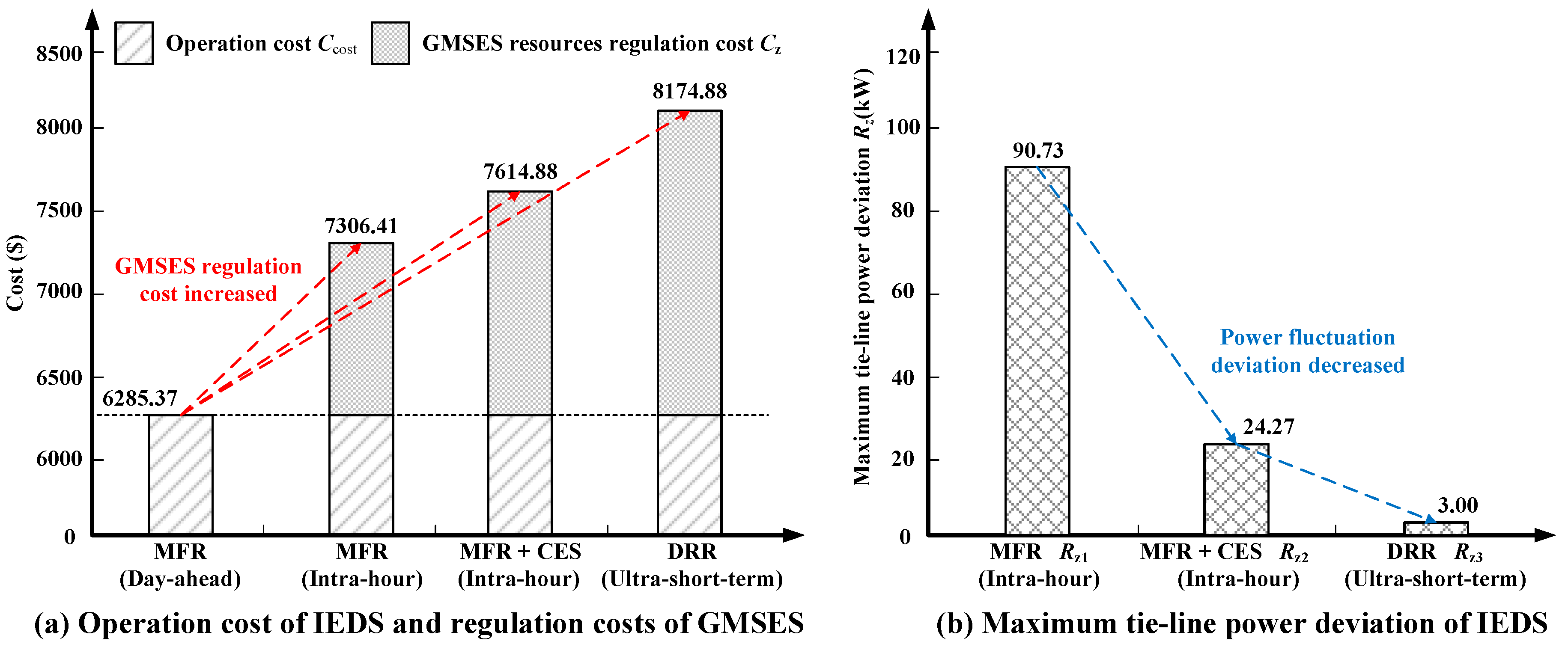
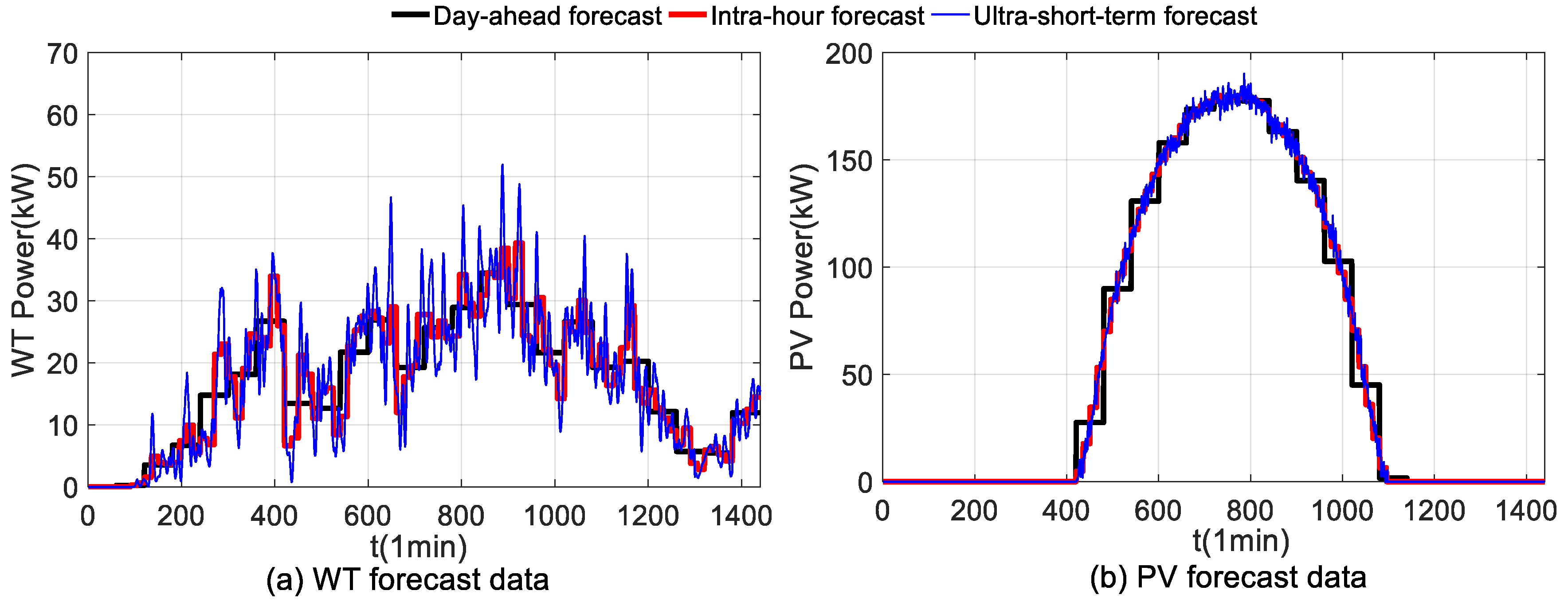
4.1. Case 1: Day-Ahead Optimal Scheduling

In the day-ahead optimal scheduling scenario, the GMSES-MFR resource is utilized to minimize the IEDS operation costs through the reasonable control of the BEH. The decoupled scenario is studied for comparison, that is to say, in the coupled nodes, the electric loads are supplied by the EPS directly, and the thermal loads are supplied by the NGS via GB. It can be concluded that the application of GMSES improves the IEDS economics. The operation costs of the IEDS decreased from $6699.21 to $6285.37, as shown in Figure 12. Furthermore, the BEH operation costs indicate a 29.62% reduction from $1397.01 to $983.16. By regulating the dispatch factors, the difference in energy prices is reflected, which shows the flexible energy supply in IEDS. The results of BEH regulation are shown in Figure 13.

Coupled units such as CHP and GB in the BEH are the physical basis for the multi-energy flow regulation. The essence of this is that the complementary characteristics and synergy effects of multi-energy flow are adopted. On the other hand, BEH can be regarded as the interface of energy coupling, and the optimal results of GMSES-MFR resources indicate the support of coupled energy sector. The excess power can be sent back to EPS when the demands of BEH are satisfied. That is to say, energy can be stored through different energy forms. The BEH consumption of natural gas is shown in Figure 13d.

The VSOC of GMSES-MFR could evaluate the state of charge and response effect towards the control signal. The VS_MFR1 is at its highest between 20:00 and 22:00 (blue line in Figure 14) due to the relatively high charging power of BEH type I, as shown in Figure 13c. However, at the same time, the VS_MFR2 is at its lowest (red line in Figure 14); this is because the output power of BEH type II is closer to its lower boundary.

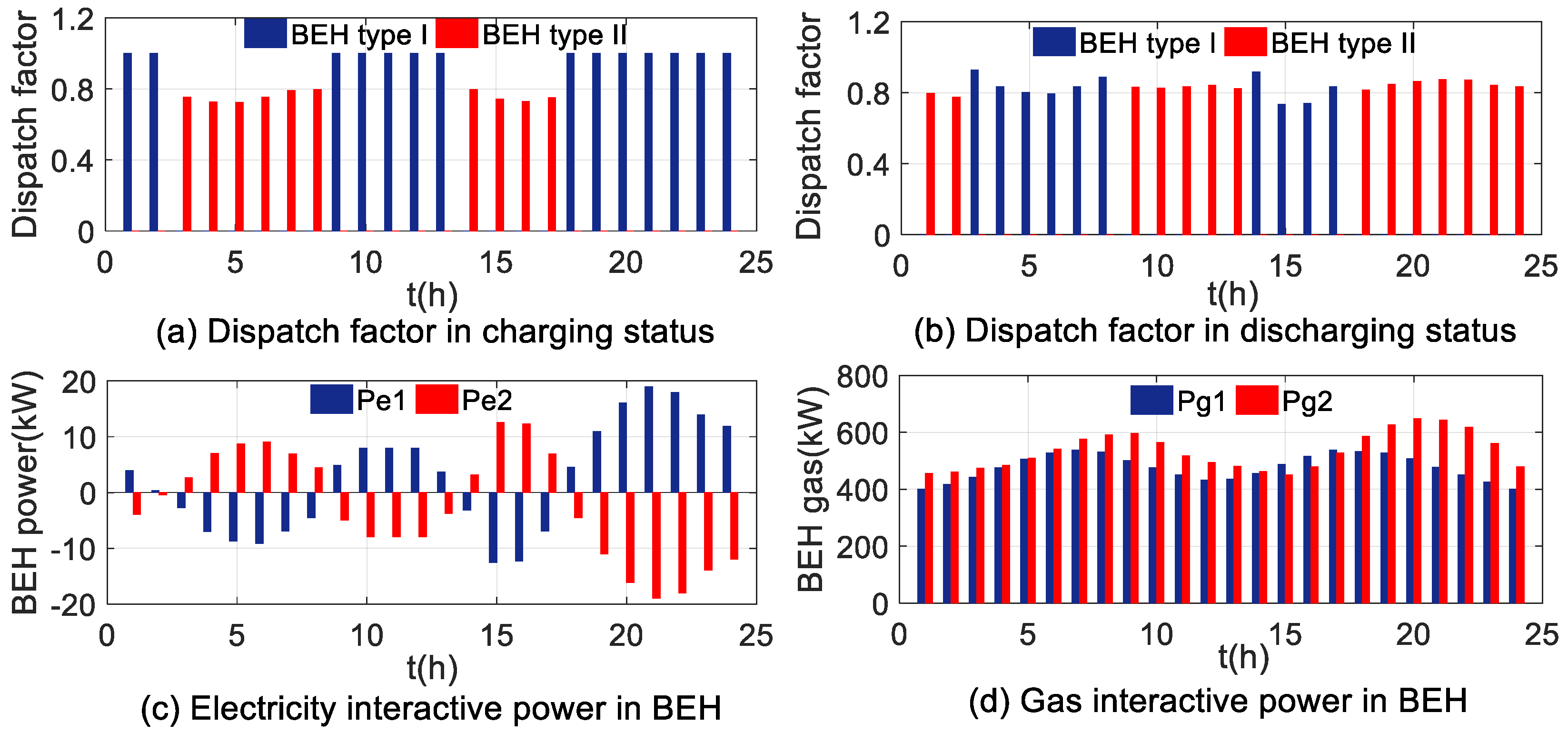
4.2. Case 2: Intra-Hour Optimal Scheduling

With the utilization of available resources of GMSES-MFR and GMSES-CES, intra-hour optimal scheduling is therefore analyzed to track the tie-line power variation in the day-ahead scenario (Case 1). The key to analyzing this issue lies in the regulatory methods in response to the control target. In addition, it is worth noting that when the combination of GMSES-MFR and GMSES-CES resources is adopted, a better control effect can be achieved, as the day-ahead tie-line power (the black line) is well tracked by Case 2 (the blue line) in Figure 15. This is because the energy conversion and dispatch of GMSES-MFR are limited due to the BEH equipment capacity, while the flexible use of GMSES-CES can compensate for the margin in power regulation. The collaborative utilization of MFR and CES could achieve a more stable control effect of the tie-line power fluctuations.

The functions of GMSES-CES are realized by regulating the SOC. As shown in Figure 16, SOC can respond to the scheduling target within the operation boundaries between 15% and 85%. Taking the period t_a as an example, when the GMSES-MFR is adopted alone, the regulated tie-line power (the red line in Figure 15) is higher than that of day-ahead scheduling baseline (the black line in Figure 15). To improve this situation, the main trend of GMSES-CES enters into the discharging status by decreasing its SOC, which facilitates the regulated tie-line power to fit the baseline. The opposite operation can be found in the period t_b. Relevant results of GMSES-MFR regulation are shown in Figure 16 and Figure 17. The integrated GMSES VSOC results are shown in Figure 18, indicating that the GMSES operation constraints are satisfied.

The power deviation is further eliminated when the GMSES-MFR and GMSES-CES resources are utilized together. However, this also brings challenges of calculating burden due to the increase of decision variables and constraints handling. Therefore, the IEDS dispatcher should select the appropriate scheduling strategies according to the target accuracy and calculation time.

4.3. Case 3: Ultra-Short-Term Energy Balance

In the ultra-short-term energy balance scenario, the GMSES-DRR is used to smooth the irregular power fluctuations under a reasonable controlling method. It is assumed that the users have signed contracts to participate in the demand response program with the IEDS. In this regard, the DRR can be fully regulated to respond to the scheduling signal. In Figure 19, a comparison about the scheduling results in cases mentioned above suggests that the tie-line power fluctuations are well smoothed by the GMSES-DRR. A few fluctuations show up because the DRR target has reached its regulation boundaries. The application of the general parameter serialization (GPS)-based control strategy has caused GMSES-DRR to provide the required power increase or decrease. In addition, based on the response characteristics of each controllable element, GMSES-DRR can be well controlled to respond to minute-level power fluctuations within operation boundaries in Figure 20.

With these operation constraints, the VSOC results of GMSES-DRR are shown in Figure 21. It can be seen that the CAC power is highest between 8:00 and 18:00 in Figure 20, which comprises most of the total output power of DRR. As a result, the VSOC of DRR becomes the highest in Figure 21, indicating that the virtual stored energy is almost full.

In addition, to measure the smoothing effect of tie-line power fluctuations, the tie-line power control error err_z and the tie-line power deviation R_z are defined in Equations (42) and (43).

$$er{r}_{z,t}=\frac{P_{\mathrm{ex},t}^{\mathrm{set}}-P_{\mathrm{ex},t}^z}{P_{\mathrm{ex},t}^{\mathrm{set}}}\times 100\%\forall t\in {\mathrm{T}}^{″}$$

(42)

$$R_{z,t}=\left|P_{\mathrm{ex},t}^z-P_{\mathrm{ex},t}^{\mathrm{set}}\right|\forall t\in {\mathrm{T}}^{″}$$

(43)

where z is the application scenario, including intra-hour scheduling (using GMSES-MFR only), Case 2 (using GMSES-MFR and GMSES-CES), and Case 3 (using GMSES-DRR); $P_{\mathrm{ex},t}^z$ is the tie-line power under the application scenario z at the tth minute. The tie-line power control error err_z under the above scenario is shown in Figure 22.

In Figure 22, it can be concluded that the tie-line power control error decreases from the use of GMSES-MFR, GMSES-MFR and GMSES-CES, to GMSES-DRR. The correction of power fluctuations for the updated data in the ultra-short-term is the best. In addition to the tie-line power, the operation and regulation costs of IEDS are shown in Figure 23a, which is essential to guaranteeing accurate IEDS operation. The GMSES regulation costs C_z, composed of C_z1, C_z2, C_z3, are calculated by Equations (44)–(46).

$$C_{\mathrm{z}1}={\displaystyle \sum _{t=1}^{{\mathrm{T}}^{\prime }}(\frac{{\pi }_{\mathrm{e}-\mathrm{buy},t}+{\pi }_{\mathrm{e}-\mathrm{sell},t}}{2}{P}_{\mathrm{e},t}^{\mathrm{z}1}+\frac{{\pi }_{\mathrm{e}-\mathrm{buy},t}-{\pi }_{\mathrm{e}-\mathrm{sell},t}}{2}\left|P_{\mathrm{e},t}^{\mathrm{z}1}\right|+{\pi }_{\mathrm{g},t}{P}_{\mathrm{g},t}^{\mathrm{z}1})}\forall t\in {\mathrm{T}}^{\prime }$$

(44)

$$C_{\mathrm{z}2}={\displaystyle \sum _{t=1}^{{\mathrm{T}}^{\prime }}(\frac{{\pi }_{\mathrm{e}-\mathrm{buy},t}+{\pi }_{\mathrm{e}-\mathrm{sell},t}}{2}{P}_{\mathrm{e},t}^{\mathrm{z}2}+\frac{{\pi }_{\mathrm{e}-\mathrm{buy},t}-{\pi }_{e-\mathrm{sell},t}}{2}\left|P_{\mathrm{e},t}^{\mathrm{z}2}\right|+{\pi }_{\mathrm{g},t}{P}_{\mathrm{g},t}^{\mathrm{z}2}+{\pi }_{\mathrm{CES}}\left|P_{\mathrm{CES},t}^{\mathrm{z}2}\right|)}\forall t\in {\mathrm{T}}^{\prime }$$

(45)

$$C_{\mathrm{z}3}={\displaystyle \sum _{t=1}^{{\mathrm{T}}^{″}}({\displaystyle \sum _{m=1}^{\mathrm{M}}{C}_m·{\beta }_m^t·\left|P_m^{t-1}-P_{\mathrm{m},\mathrm{tar}}^t\right|})}\forall t\in {\mathrm{T}}^{″}$$

(46)

where $C_{\mathrm{z}1}$, $C_{\mathrm{z}2}$, $C_{\mathrm{z}3}$ represent the GMSES regulation cost of using MFR, using MFR and CES (Case 2), and using DRR (Case 3) in a day respectively; ${\pi }_{\mathrm{CES}}$ is the regulation cost of using CES; $P_{\mathrm{CES},t}^{\mathrm{z}2}$ is the charging and discharging power in Case 2 at period t.

The GMSES regulation costs increase as the response resource varies from MFR to DRR, as shown in Figure 23a. However, it is worth pointing out that the tie-line power deviation is decreased, reducing the influence of the underlying IEDS on the upper energy system. The fluctuations of renewable energy and loads are accommodated by GMSES resources and the relevant energy scheduling strategy, which contributes to stable operation, as well as improving the power quality. In the ultra-short-term energy balance, although the regulation cost of using DRR is high, the tie-line power deviation reaches its lowest value (depicted in Figure 23b). This is because the regulation cost of per-unit DRR is relatively high, and DRR is regulated frequently. On the other hand, due to the real-time coordination and regulation of DRR, the aperiodic power fluctuations of the renewable energy and loads could be smoothed out.

In summary, the three kinds of resources in GMSES should be applied in different scenarios owing to their response characteristics and application demands. Specifically, the GMSES-MFR could be used in day-ahead optimal scheduling, such as economic scheduling and loss reduction. The GMSES-MFR and GMSES-CES are suitable for intra-hour scheduling with relatively high adjustment accuracy. As for the ultra-short-term energy balance, the GMSES-DRR can be selected to meet high-precision requirement with sufficient regulation costs and calculating time.

5. Conclusions

This paper proposes a generalized multi-source energy storage (GMSES) model that includes resources of conventional energy storage, multi-energy flow and demand response. Aggregation and coordination of GMSES resources show the potential of equivalent energy storage, where investment in conventional energy storage can be reduced. Uncertainties in the renewable energy and energy loads bring challenges to IEDS operation on multiple time scales. To solve this problem, the GMSES hierarchical optimal scheduling framework is studied, including day-ahead, intra-hour, and ultra-short-term scheduling. To be specific, operation costs are minimized in day-ahead scheduling due to the complementary nature of multi-carrier energy prices, and the set-points can be generated, as well as the basic tie-line power. Various GMSES resources are called upon in both intra-hour scheduling and the ultra-short-term scenario, where power deviation caused by forecast error can be regulated, and energy balance service can be provided.

It is worth mentioning that the general parameter serialization (GPS)-based control strategy was studied to determine the responsive group and priority sequence in ultra-short-term scheduling. Demand response resources (including heat pumps, central air conditioning and electric vehicles) can be integrated in a flexible way for power fluctuation smoothing.

The proposed hierarchical scheduling strategy is conducted in a modified electricity-gas coupled IEDS. Numerical results have shown the effectiveness of the co-optimization GMSES model in reducing the impacts on the upper layer energy system; in addition, the operation costs and the tie-line power fluctuations can be minimized by GMSES. The comparison of GMSES resources is given through the scheduling results, showing the applicability and scalability in multi-type multi-timescale regulation, which contributes to the decision making of IEDS dispatch center.

References

1. Wen, S.; Lan, H.; Fu, Q.; Yu, D.C.; Zhang, L. Economic allocation for energy storage system considering wind power distribution. IEEE Trans. Power Syst. 2015, 30, 644–652. [Google Scholar] [CrossRef]
2. He, G.; Chen, Q.; Kang, C.; Xia, Q.; Poolla, K. Cooperation of wind power and battery storage to provide frequency regulation in power markets. IEEE Trans. Power Syst. 2017, 32, 3559–3568. [Google Scholar] [CrossRef]
3. Ibrahim, H.; Ilinca, A.; Perron, J. Energy storage systems--characteristics and comparisons. Renew. Sustain. Energy Rev. 2008, 12, 1221–1250. [Google Scholar] [CrossRef]
4. Singh, S.; Singh, M.; Kaushik, S.C. Feasibility study of an islanded microgrid in rural area consisting of PV, wind, biomass and battery energy storage system. Energy Convers. Manag. 2016, 128, 178–190. [Google Scholar] [CrossRef]
5. European commission. Strategic energy technologies [online]. 2013. Available online: http://setis.ec.europa.eu/technologies (accessed on 14 August 2018).
6. Zito, R. Energy Storage; John Wiley & Sons: Hoboken, NJ, USA, 2013. [Google Scholar]
7. Zhao, H.; Wu, Q.; Hu, S.; Xu, H.; Rasmussen, C.N. Review of energy storage system for wind power integration support. Appl. Energy 2015, 137, 545–553. [Google Scholar] [CrossRef] [Green Version]
8. Lott, M.C.; Kim, S.I.; Tam, C.; Houssin, D.; Gagné, J.F. Technology Roadmap: Energy Storage; International Energy Agency: Paris, France, 2014. [Google Scholar]
9. Chen, H.; Cong, T.N.; Yang, W.; Tan, C.; Li, Y.; Ding, Y. Progress in electrical energy storage system: A critical review. Prog. Nat. Sci. 2009, 19, 291–312. [Google Scholar] [CrossRef]
10. Chen, J.Z.; Liao, W.Y.; Hsieh, W.Y.; Hsu, C.C.; Chen, Y.S. All-vanadium redox flow batteries with graphite felt electrodes treated by atmospheric pressure plasma jets. J. Power Sources 2015, 274, 894–898. [Google Scholar] [CrossRef]
11. Jacob, A.S.; Banerjee, R.; Ghosh, P.C. Sizing of hybrid energy storage system for a PV based microgrid through design space approach. Appl. Energy 2018, 212, 640–653. [Google Scholar] [CrossRef]
12. Reihani, E.; Motalleb, M.; Thornton, M.; Ghorbani, R. A novel approach using flexible scheduling and aggregation to optimize demand response in the developing interactive grid market architecture. Appl. Energy 2016, 183, 445–455. [Google Scholar] [CrossRef]
13. Cole, W.J.; Marcy, C.; Krishnan, V.K.; Margolis, R. Utility-scale lithium-ion storage cost projections for use in capacity expansion models. In Proceedings of the North American Power Symposium (NAPS), Denver, CO, USA, 18–20 September 2016; pp. 1–6. [Google Scholar]
14. Wang, D.; Liu, L.; Jia, H.; Wang, W.; Zhi, Y.; Meng, Z.; Zhou, B. Review of key problems related to integrated energy distribution systems. CSEE J. Power Energy Syst. 2018, 4, 130–145. [Google Scholar] [CrossRef]
15. Li, G.; Zhang, R.; Jiang, T.; Chen, H.; Bai, L.; Cui, H.; Li, X. Optimal dispatch strategy for integrated energy systems with CCHP and wind power. Appl. Energy 2017, 192, 408–419. [Google Scholar] [CrossRef]
16. Li, Y.; Zou, Y.; Tan, Y.; Cao, Y.; Liu, X.; Shahidehpour, M.; Tian, S.; Bu, F. Optimal stochastic operation of integrated low-carbon electric power, natural gas, and heat delivery system. IEEE Trans. Sustain. Energy 2018, 9, 273–283. [Google Scholar] [CrossRef]
17. Song, H.; Yu, G.; Qu, Y. Web of cell architecture-new perspective for future smart grids. Autom. Electr. Power Syst. 2017, 41, 1–9. [Google Scholar]
18. Javadi, M.; Marzband, M.; Funsho Akorede, M.; Godina, R.; Saad Al-Sumaiti, A.; Pouresmaeil, E. A centralized smart decision-making hierarchical interactive architecture for multiple home microgrids in retail electricity market. Energies 2018, 11, 3144. [Google Scholar] [CrossRef]
19. Valinejad, J.; Marzband, M.; Funsho Akorede, M.; D Elliott, I.; Godina, R.; Matias, J.; Pouresmaeil, E. Long-term decision on wind investment with considering different load ranges of power plant for sustainable electricity energy market. Sustainability 2018, 10, 3811. [Google Scholar] [CrossRef]
20. Wang, W.; Wang, D.; Jia, H.; Zhi, Y.; Liu, L.; Fan, M.; Lin, J. Economic dispatch of generalized multi-source energy storage in regional integrated energy systems. Energy Procedia 2017, 142, 3270–3275. [Google Scholar] [CrossRef]
21. Wang, Z.; Chen, B.; Wang, J.; Begovic, M.M.; Chen, C. Coordinated energy management of networked microgrids in distribution systems. IEEE Trans. Smart Grid 2015, 6, 45–53. [Google Scholar] [CrossRef]
22. Valinejad, J.; Barforoshi, T.; Marzband, M.; Pouresmaeil, E.; Godina, R.; PS Catalão, J. Investment incentives in competitive electricity markets. Appl. Sci. 2018, 8, 1978. [Google Scholar] [CrossRef]
23. Tavakoli, M.; Shokridehaki, F.; Marzband, M.; Godina, R.; Pouresmaeil, E. A two stage hierarchical control approach for the optimal energy management in commercial building microgrids based on local wind power and PEVs. Sustain. Cities Soc. 2018, 41, 332–340. [Google Scholar] [CrossRef]
24. Wu, X.; Wang, X.; Qu, C. A hierarchical framework for generation scheduling of microgrids. IEEE Trans. Power Deliv. 2014, 29, 2448–2457. [Google Scholar] [CrossRef]
25. Sami, S.S.; Cheng, M.; Wu, J. Modelling and control of multi-type grid-scale energy storage for power system frequency response. In Proceedings of the 2016 IEEE 8th International Power Electronics and Motion Control Conference (IPEMC-ECCE Asia), Hefei, China, 22–26 May 2016; pp. 269–273. [Google Scholar]
26. Dugan, R.C.; Taylor, J.A.; Montenegro, D. Energy storage modeling for distribution planning. IEEE Trans. Ind. Appl. 2017, 53, 954–962. [Google Scholar] [CrossRef]
27. Xu, X.; Jin, X.; Jia, H.; Yu, X.; Li, K. Hierarchical management for integrated community energy systems. Appl. Energy 2015, 160, 231–243. [Google Scholar] [CrossRef]
28. Liu, Y.; Zhang, Y.; Chen, K.; Chen, S.Z.; Tang, B. Equivalence of multi-time scale optimization for home energy management considering user discomfort preference. IEEE Trans. Smart Grid 2017, 8, 1876–1887. [Google Scholar] [CrossRef]
29. Belderbos, A.; Delarue, E.; D’haeseleer, W. Possible role of power-to-gas in future energy systems. In Proceedings of the 2015 12th International Conference on the European Energy Market (EEM), Lisbon, Portugal, 19–22 May 2015; pp. 1–5. [Google Scholar]
30. Ahern, E.P.; Deane, P.; Persson, T.; Gallachóir, B.Ó.; Murphy, J.D. A perspective on the potential role of renewable gas in a smart energy island system. Renew. Energy 2015, 78, 648–656. [Google Scholar] [CrossRef]
31. Liu, D.; Li, H. A ZVS bi-directional DC–DC converter for multiple energy storage elements. IEEE Trans. Power Electron. 2006, 21, 1513–1517. [Google Scholar] [CrossRef]
32. Wang, W.; Wang, D.; Jia, H.; Chen, Z.; Tang, J. A decomposed solution of multi-energy flow in regional integrated energy systems considering operational constraints. Energy Procedia 2017, 105, 2335–2341. [Google Scholar] [CrossRef]
33. Kandasamy, N.K.; Tseng, K.J.; Boon-Hee, S. Virtual storage capacity using demand response management to overcome intermittency of solar PV generation. IET Renew. Power Gener. 2017, 11, 1741–1748. [Google Scholar] [CrossRef]
34. Liu, K.; Yang, W.; Wang, D.; Jia, H.; Gui, H.; Song, Y.; Fan, M. Reaearch on renewable energy scheduling and node aggregrated demand response strategy based on distribution network power flow tracking. Proc. CSEE 2018, 38, 5714–5726. [Google Scholar]
35. Lu, N.; Chassin, D.P. A state-queueing model of thermostatically controlled appliances. IEEE Trans. Power Syst. 2004, 19, 1666–1673. [Google Scholar] [CrossRef]
36. Arvesen, Ø.; Medbø, V.; Fleten, S.E.; Tomasgard, A.; Westgaard, S. Linepack storage valuation under price uncertainty. Energy 2013, 52, 155–164. [Google Scholar] [CrossRef] [Green Version]
37. Houwing, M.; Negenborn, R.R.; De Schutter, B. Demand response with micro-CHP systems. Proc. IEEE 2011, 99, 200–213. [Google Scholar] [CrossRef]
38. Dugan, R.C.; McDermott, T.E. An open source platform for collaborating on smart grid research. In Proceedings of the 2011 IEEE Power and Energy Society General Meeting, Detroit, MI, USA, 24–29 July 2011; pp. 1–7. [Google Scholar]
39. Tang, J.; Wang, D.; Wang, X.; Jia, H.; Wang, C.; Huang, R.; Yang, Z.; Fan, M. Study on day-ahead optimal economic operation of active distribution networks based on Kriging model assisted particle swarm optimization with constraint handling techniques. Appl. Energy 2017, 204, 143–162. [Google Scholar] [CrossRef]
40. Negash, A.I.; Haring, T.W.; Kirschen, D.S. Allocating the cost of demand response compensation in wholesale energy markets. IEEE Trans. Power Syst. 2015, 30, 1528–1535. [Google Scholar] [CrossRef]
41. Wang, W.; Wang, D.; Jia, H.; He, G.; Hu, Q.E.; Sui, P.C.; Fan, M. Performance evaluation of a hydrogen-based clean energy hub with electrolyzers as a self-regulating demand response management mechanism. Energies 2017, 10, 1211. [Google Scholar] [CrossRef]
42. Pacific Gas & Electrc. Available online: http://www.pge.com/tariffs/electric.shtml (accessed on 16 August 2018).
Figure 1. Functional applications of energy storage systems (ESSs) and generalized multi-source energy storage (GMSES) [6,7].
Energies 12 00246 g001
Figure 2. Functional framework of generalized multi-source energy storage (GMSES).
Energies 12 00246 g002
Figure 3. Illustration of the GMSES-MFR: (a) charging/standby status, (b) discharging status.
Energies 12 00246 g003
Figure 4. Operation characteristics of GMSES-DRR.
Energies 12 00246 g004
Figure 5. Controlled logic diagram of the general parameter serialization (GPS)-based control strategy.
Energies 12 00246 g005
Figure 6. Flowchart of the general parameter serialization (GPS)-based control strategy.
Energies 12 00246 g006
Figure 7. Hierarchical scheduling framework of GMSES.
Energies 12 00246 g007
Figure 8. Flowchart of hierarchical optimal scheduling algorithm.
Energies 12 00246 g008
Figure 9. Flowchart of DRR control strategy algorithm.
Energies 12 00246 g009
Figure 10. Topology of IEDS based on GMSES.
Energies 12 00246 g010
Figure 11. Illustration of the GMSES-DRR.
Energies 12 00246 g011
Figure 12. Results of day-ahead optimal scheduling.
Energies 12 00246 g012
Figure 13. Illustration of BEH regulation results in Case 1.
Energies 12 00246 g013
Figure 14. Results of VSOC of GMSES-MFR.
Energies 12 00246 g014
Figure 15. Tie-line power fluctuations smoothing results in the intra-hour scenario.
Energies 12 00246 g015
Figure 16. Results of GMSES-CES SOC and GMSES-MFR VSOC.
Energies 12 00246 g016
Figure 17. BEH regulation results in Case 2.
Energies 12 00246 g017
Figure 18. Results of integrated GMSES VSOC.
Energies 12 00246 g018
Figure 19. Tie-line power fluctuations smoothing results.
Energies 12 00246 g019
Figure 20. The response results of DRRs.
Energies 12 00246 g020
Figure 21. Results of GMSES-DRR VSOC.
Energies 12 00246 g021
Figure 22. Tie-line power control error results.
Energies 12 00246 g022
Figure 23. (a) Operation cost of IEDS and regulation costs of GMSES; (b) maximum tie-line power deviation of IEDS.
Energies 12 00246 g023