Abstract
Pressure-retarded osmosis (PRO) is viewed as a highly promising renewable energy process that generates energy without carbon emissions in the age of the climate change regime. While many experimental studies have contributed to the quest for an efficiency that would make the PRO process commercially viable, computational modeling and simulation studies have played crucial roles in investigating the efficiency of PRO, particularly the concept of hybridizing the PRO process with reverse osmosis (RO). It is crucial for researchers to understand the implications of the simulation and modeling works in order to promote the further development of PRO. To that end, the authors collected many relevant papers and reorganized their important methodologies and results. This review, first of all, presents the mathematical derivation of the fundamental modeling theories regarding PRO including water flux and concentration polarization equations. After that, those theories and thermodynamic theories are then applied to depict the limitations of a stand-alone PRO process and the effectiveness of an RO-PRO hybridized process. Lastly, the review diagnoses the challenges facing PRO-basis processes which are insufficiently resolved by conventional engineering approaches and, in response, presents alternative modeling and simulation approaches as well as novel technologies.
1. Introduction
The force of climate change is becoming more apparent as the temperature of the earth continues to break records, farmlands are ruined by abnormally low rainfall, and the fury of extreme weather grows increasingly life-threatening [1,2]. Climate change is depleting resources that are indispensable for human life such as water while highlighting the importance of renewable energy sources. In the face of these crises, membrane-based desalting processes are regarded as effective alternatives to confront the need for water and alternative energy in the age of the climate change regime. Membrane-based desalting processes that aim to produce freshwater are already contributing to relieving water shortages around the world. Out of many desalination processes, reverse osmosis (hereafter abbreviated as RO) is the most widely used. Meanwhile, another type of membrane-based desalting process that generates energy by mixing two sorts of differently concentrated liquids is being used to meet energy needs. Pressure-retarded osmosis (hereafter abbreviated as PRO) is regarded as the exemplar of this type of membrane-based desalting process.
The objective of PRO is to generate electricity using a salinity gradient by mixing two types of differently concentrated solutions such as seawater and river water. Given that the amount of seawater around the globe is immense, the PRO process has a high potential to provide a significant energy supply if satisfactory process efficiency can be attained. Moreover, the PRO process is attracting strong attention as an alternative renewable energy technology that can comply with the expectations of the current climate change regime since the process theoretically does not emit any carbon-related compounds. Encouraged by such merits of PRO, research projects related to PRO have been carried out vigorously around the globe to commercialize this process by resolving the technological problems [3]. For example, Statkraft, a renewable energy company based in Norway, ran a pilot-scale PRO process for the first time in the world in 2009 and analyzed the feasibility of the PRO process according to the operational data [4,5]. Thereafter, many countries began to develop PRO-related technologies, among them the global MVP project in the Republic of Korea and the Megaton project in Japan [6,7,8].
While the PRO process has achieved appreciable technological advances in a number of research projects, nevertheless, several obstacles still hamper the commercialization of the process. For example, multiple types of research concluded that a stand-alone PRO process was not viable due to the inherent thermodynamic limits [9,10,11,12] and the vulnerability of a membrane to the fouling propensity [13,14,15,16,17,18,19]: the inherent thermodynamic limits and the vulnerability of a membrane to the fouling propensity will be elaborated in the upcoming sections.
To compensate for the aforementioned limits and to stabilize the supply of water and energy around the world simultaneously, a concept of hybridization that combines the PRO process with other desalination processes has been widely applied in this field. By applying the hybridization strategy to PRO, the vulnerability of a PRO membrane to fouling can be mitigated because of pretreatment deployed prior to a desalination process. Furthermore, the energy consumed by a desalination process can be recovered partially by a PRO process [13,14]. Due to these advantages, PRO hybridized processes were rapidly seen as a promising process type. In particular, an RO-PRO hybridized process became the most popular since RO is most widely implemented desalination process today.
Nevertheless, the RO-PRO hybridized process is far from maturation: technological discrepancies between the RO and PRO processes are so vast that implementing an RO-PRO plant is quite a task. Therefore, a series of simulation and modeling studies are imperative to analyze and improve the efficiency of the RO-PRO process. To that end, hundreds of research papers regarding the simulation and modeling of PRO-hybridized processes have been published thus far. For example, some researchers such as Khaled Touati attempted to combine a PRO process with conventional thermal desalination processes (e.g., multi-effect distillation) and to test the feasibility of the hybridized processes with a numerical analysis approach [20,21]. Meanwhile, some researchers such as Wei He had sought to maximize the efficiency of a PRO process by connecting the stand-alone PRO processes in series [22,23]. There were also other novel approaches expanding the scale of a PRO-hybridized process such as RO-membrane distillation-PRO [24,25]. However, most of the papers related to PRO-hybridized processes are dedicated to the RO-PRO process. The aforementioned new attempts are just expanded versions of RO-PRO. So a more complete understanding of the RO-PRO process should supersede the consideration of other hybridized processes.
The objective of this review is to survey the current status of PRO process technology and ultimately provide a prospect for the PRO-hybridized process which is represented by the RO-PRO process, by reflecting the important methodologies and results from relevant computational modeling and simulation studies. To do so, this review first introduces mathematical theories of stand-alone PRO which are imperative for understanding PRO-basis processes. The subsequent section elaborates on the viability limit of a stand-alone PRO process and the hybridization features in an RO-PRO process, using the thermodynamic theories and the fundamental theories introduced in the first section. In the last section, the major challenges to the PRO-basis process, which are insufficiently resolved by conventional engineering approaches, are considered, and novel technologies that can cope with the major challenges are addressed.
2. Fundamental Theories for a PRO Process
As is widely known, there are three broad categories of membrane-based desalting processes, consisting of forward osmosis (FO), RO, and PRO (Figure 1). FO is a process that utilizes the phenomenon of osmosis as it exists in nature: i.e., the solvent of a lower-solute concentration solution naturally shifts towards a higher-solute concentration solution until the concentration of the latter decreases. RO is a process that utilizes the opposite mechanism: in RO, external hydraulic pressure sufficiently higher than the osmotic pressure is applied to a highly concentrated solution. The external hydraulic pressure forces freshwater in a more highly concentrated solution to cross a membrane by leaving solutes behind. When examining the mechanisms of FO and RO, it is apparent that the objectives of the processes are to dilute a more concentrated solution or to produce freshwater.
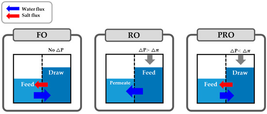
Figure 1.
The schematic figures illustrating the mechanisms of forward osmosis (FO), reverse osmosis (RO), and pressure-retarded osmosis (PRO).
The objective of PRO is quite different from that of FO and RO. Whereas FO and RO focus on producing clean water, PRO mainly focuses on generating electricity using a salinity gradient. An operational mechanism of PRO is an intermediate form between FO and RO. That is, in PRO, an external hydraulic pressure is applied to a more highly concentrated solution usually called a draw solution (hereafter, the draw solution will refer to that of a PRO process unless otherwise noted). However, the solvent of a less concentrated solution, usually called a feed solution (feed solution hereinafter refers to that of a PRO process unless noted) also shifts towards a higher concentrated solution simultaneously (Figure 1). In short, a higher-solute concentration solution such as seawater draws a lower-solute concentration solution when an external hydraulic pressure is applied. The pressurized solution that has drawn a lower solution now attains the potential power for generating electricity. After that, the pressurized solution serves as an energy source and the potential power turns into the mechanical energy due to an energy converter such as a hydro turbine or an energy exchanger. That is, the potential power in the pressurized solution is ‘harvested’ by the energy converter and the PRO can generate the electricity.
In this section, for a clear understanding, the fundamental models mathematically describing the energy-generating procedures in PRO will be elaborated with detailed derivation steps.
2.1. Water Flux and Power Density
Now let us introduce mathematical notations and equations. The most fundamental and common equation for membrane-based desalting processes regardless of types is the van’t Hoff equation which describes the relationship between the osmotic pressure () and the solute concentration of the solution (), and absolute temperature (). The van’t Hoff equation is given as,
where, and indicate the van’t Hoff factor and the universal gas constant, respectively. In principle, Equation (1) only holds for the dilute solution. But for the sake of convenience, Equation (1) is assumed to be valid for a wide range of solution solute concentrations in this review. By determining the osmotic pressure based on Equation (1), a new criterion for each FO, RO, and PRO is made. A process becomes RO if the external hydraulic pressure () is higher than the osmotic pressure difference between the low-solute concentration solution and the high-solute concentration solution (). On the other hand, a process becomes FO if the external hydraulic pressure is not applied. If a process is in an intermediate form (i.e., ), then it would be PRO (Figure 2). It is necessary to understand the concepts of water flux () and power density () in order to grasp how PRO generates electricity. Water flux is a concept that is used in FO and RO as well. However, while the water flux in FO and RO is utilized to measure the produced amount of freshwater in a process, water flux in PRO is regarded as a preliminary parameter to calculate power density. Therefore, it is essential to comprehend what flux means to understand the mechanism for generating electricity in PRO. According to the solution-diffusion model, the water flux is expressed as [26]
where is the diffusion coefficient of water in the membrane and is the solute concentration according to , which is the distance from the membrane surface. Now (2) becomes (3) in accordance with the well-known Henry’s law which states that ,
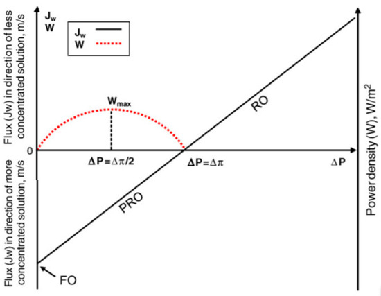
Figure 2.
A comparison of FO, PRO, and RO along with the change of external hydraulic pressure. A red-dashed parabola represents the power density of PRO according to external hydraulic pressure [30]. The figure is reproduced from Reference 30] with permission.
Here, stands for the change of water chemical potential across a membrane. can be alternatively expressed as follows, according to the definition of chemical potential,
where and indicate the chemical activity of water and partial molar volume of water. Assuming is independent of the pressure, Equation (4) becomes
A conversion of into is based on another thermodynamic definition of , which is described as [27,28]. By combining Equations (3) and (5), the last form regarding the water flux () is derived:
Ultimately, regardless of the type of membrane-based desalting process, water flux is calculated as Equation (6). Note that signs for the hydraulic pressure and the osmotic pressure in PRO are switched because the osmotic pressure is always higher than the hydraulic pressure in PRO. If a set of parameters () on the right-hand side of Equation (6) are replaced with , as in
Then, Equation (7) is the most basic water flux model used in a PRO-basis process. Here, is one of the membrane parameters in membrane-based desalting processes, which is called the water permeability. The water permeability implies how much water flux can be measured per unit of external pressure (the unit of water permeability is a ratio of the water flux to the pressure). This is one of the important parameters that indicates the performance of the membrane together with salt permeability () and membrane structure parameter (). Meanwhile, the second term on the right-hand side of (7), , denotes the net driving pressure of membrane-based desalting processes. By multiplying this term with the water permeability, the flux of water permeated across a membrane is calculated.
A physical meaning of water flux is the volumetric rate of fresh water permeated per unit membrane area (). In a PRO process, the water flux is directly related to a process index, . is an indicator meaning how much energy is generated per unit time and per unit membrane area: thus, it can be interpreted as a kind of energy flux (). in PRO is defined as
By substituting Equation (7) into Equation (8), an equation is obtained as follows:
If the osmotic pressure of each solution (i.e., a more highly concentrated solution and a less concentrated solution) is constant, then Equation (9) becomes a quadratic function with respect to the external hydraulic pressure. Now Equation (9) should be differentiated in order to find the maximum value of under the given condition. By doing so, a relation between and for the maximum is found as follows:
In short, the of PRO is maximized when the external hydraulic pressure of PRO becomes half of the osmotic pressure difference. By combining Equation (9) and Equation (10), the maximum is calculated as [29,30],
It is instructive for readers to remember this criterion because it is frequently used to design an optimal PRO process. In Figure 2, a red-dashed parabola depicts how varies according to the external hydraulic pressure. Since the objective of PRO is to generate electricity, the external hydraulic pressure must maintain its own range between zero and the osmotic pressure difference.
2.2. Water Flux with Concentration Polarization Phenomena
In a previous subsection, the water flux for PRO was derived as given in (7). One should note that the water flux is based on an ideal assumption that is only represented by the solute concentration difference between the bulk feed solution ( and bulk draw solution (. Although such an ideal assumption often provides convenience in observing the overall tendency of a PRO process, the values resulting from the water flux with an ideal assumption are usually incorrect due to the lack of the reflection of the concentration polarization. Concentration polarization (CP) is a phenomenon which is led by an encounter between the water flux and the salt flux, occurring in the inside and near-outside of a membrane. To understand CP, the basic transport phenomena around a membrane first should be acknowledged.
2.2.1. Internal Concentration Polarization
As the solvents in the solution travel across a membrane, the solutes in the solution cross a membrane due to the solute concentration difference between the feed and draw sides. This phenomenon of solute transport across a membrane is called salt flux. The physical meaning of salt flux is the mass rate of solute penetrating per unit membrane area (. Understanding the factor of salt flux is imperative for understanding the system dynamics and CP in membrane-based desalting processes. As shown in Figure 3, the water flux and the salt flux in a PRO system, as well as in a FO system, tend to flow in opposite directions.
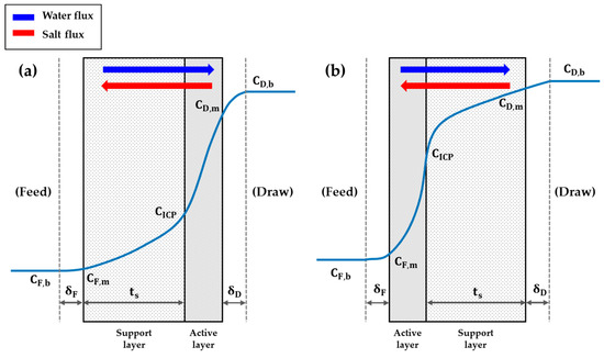
Figure 3.
The structure of a PRO membrane of (a) which an active layer faces a draw solution side, and (b) of which a support layer faces a draw solution.
That is, while the water flux in a PRO system tends to stream from the feed side to the draw side, the salt flux streams from the draw side to the feed side. This contrary tendency results from the difference of media which drive the flow of each flux. The opposite directions of each flux, first of all, result in the isolation of salts inside a membrane—imagine a situation in which the salts try to reach the feed side but fail because of the water flux serving as shoving the salts back to the draw side. Consequently, some amounts of salts are stranded in a membrane permanently and form a new concentration located inside a membrane, . This phenomenon is called internal concentration polarization (ICP). ICP is one of the major burdens imposed on FO and PRO processes, as it strongly aggravates the performance of those processes. As ICP is taken into consideration, the substantial osmotic pressure difference changes from the one estimated with and to the one estimated with and . Such a change in the substantial osmotic pressure difference is directly linked to the decrease in the driving force. Naturally, the performance of a PRO process decreases, as well. If the composition of solutes is not just confined to a pure salt, the impact of ICP grows even larger. As the composition of solutes gets intricate, the interactions among the solute compounds or organisms aggravate the performance of a membrane. For example, the microbes in the feed and draw solutions produce byproducts such as polysaccharides and proteins [13]. Such byproducts get accumulated inside a membrane and result in a severer ICP. In addition, the increased microbes also clog the pores in a membrane so that the performance of a process essentially goes down. One of the ways to relieve such an impact of fouling propensity worsened by ICP is to switch the membrane orientation [13,31]. A PRO process usually sets the membrane orientation of a system as Figure 3a, which is called the AL-DS (Active Layer–Draw Solution) mode, due to its higher initial water flux than that of Figure 3b, which is called the AL-FS (Active Layer–Feed Solution) mode [32,33]. However, the AL-DS mode is more vulnerable to the fouling propensity incurred inside a membrane than the AL-FS mode since the porous structure of the support layer plays a role to trap the foulants from the feed solution more sensitively [34]. Therefore, while the same amount of foulants is accumulated on the surface of a membrane, the water flux in the AL-DS mode declines more rapidly than that in the AL-FS mode [13,31]. However, a sequence in which ICP induces the fouling further or the fouling induces ICP further depends on the composition of foulants in the raw water [13,17,35,36]. Thus, an operator should choose whether to apply the AL-DS mode or the AL-FS mode for a given system in accordance with the compound composition of the intake water. As the orientation of a PRO membrane is switched, the equations of the models are also slightly changed since the solute concentration distribution inside a membrane changes. In the current paper, the equations of the AL-FS mode will not be represented additionally because most of the research works regarding a PRO process are based on the AL-DS mode.
ICP is an inevitable phenomenon in the FO and PRO processes since the directions of water flux and salt flux in the processes are always oriented reversely. To analyze ICP mathematically, the mathematical expression of the salt flux should be noted first [37,38].
Here, , , , and represent the salt flux, the salt permeability, the solute concentration of the draw solution at the adjacent area of the membrane, and the solute concentration of feed solution at the adjacent area of the membrane, respectively. Lee et al. [37] developed a theoretical model for the PRO process based on the conservation of the mass resulting from the water flux and the salt flux. Assuming, for the sake of simplicity, that there is only one solute (i.e., salt) in the draw solution, the mass transfer of the salt entering the membrane support layer at each boundary layer is always equal to the sum of the salinity displacement due to convection and diffusion caused by the salinity difference. Thus, at a steady-state, the conservation of mass in a system can be described as follows, [39]
As noted in a previous subsection, is the solute concentration at position ; and is the diffusion coefficient at the support layer of a membrane (Figure 3), which is defined as [40],
Here, is the diffusion coefficient, which is commonly referred to as diffusivity, in the bulk solution; is the porosity of the support layer; and is the tortuosity of the support layer. A detailed description of these parameters will be covered a bit later. By rearranging Equation (13) appropriately, the following relation is derived,
If (15) is integrated along with the boundary conditions shown in Equation (16), the solute concentration of ICP () comes out as given in Equation (17) [14],
where is the distance from the support layer to the active layer boundary; and is the thickness of the support layer of a membrane (Figure 3). A new term that emerges in Equation (17), , represents the solute resistivity in the support layer and is defined as [41]
As shown in Equation (18), is generally expressed as , structure parameter. As mentioned before, three membrane parameters, (water permeability), (salt permeability), and (structure parameter), are considered the main parameters displaying the properties of a membrane. The roles of and are relatively clear. In order to enhance the performance of a system, the operators of a PRO process should increase the water flux by augmenting the value of as much as possible: see Equation (7). In the meantime, the salt flux should be decreased as much as possible, so that the value of must be repressed: see Equation (12). However, understanding the role of is a bit more complicated than understanding those of and . When considering Equation (18), it is apparent that is proportional to the value of . Considering that increases as increases, the value of should be kept minimal to maintain a high substantial osmotic pressure difference. However, the reduction of must be in a balance with the tortuosity and the thickness of the support layer because excessively low values of those terms can have harmful impacts on the mechanical strength of a membrane. In short, recalling that , the thickness of the support layer and the tortuosity should be as low as possible while the porosity is kept high. Therefore, satisfying these features should be the priority when fabricating a PRO membrane.
2.2.2. External Concentration Polarization
ICP is a phenomenon resulting from a lump of concentration located inside a membrane. Unlike ICP, there are two more CPs that occur outside of a membrane, known as external concentration polarization (ECP). The names of ECP differ according to regions where CP occurs. If ECP occurs at an interface region between the draw solution and a membrane, such a CP is referred to as dilutive ECP because the interface region becomes diluted by water which has crossed a membrane. By contrast, ECPs occurring at an interface region between the feed solution and a membrane is called concentrative ECP due to the impact of salt shifting from the draw side to the feed side. Much like the term ICP was derived, the terms for each ECP phenomenon are derived based upon the interaction with boundary conditions. The boundary conditions and the solute concentration at the interface region of the draw side are given as follows (Figure 3):
If the integration of Equation (15) is carried out according to the boundary conditions as in the case of ICP, then the solute concentration at the interfacial region of the membrane and the draw solution () comes as follows:
Meanwhile, the boundary conditions and the solute concentration at the interface region of the feed side are given as follows:
In the same manner, the concentration at the interfacial region of the membrane and the feed solution () can be obtained with the integration as follows:
Here, and represent the thickness of the solution boundary layer and the mass transfer coefficient, respectively. The subscripts appended to the notation each indicates a different region: subscript indicates the feed solution; the draw solution. It should be noted that the thickness of the boundary layer and mass transfer coefficient are interrelated based on the famous stagnant film theory [41,42,43,44,45],
In other words, the thickness of the solution boundary layer diminishes as the mass transfer coefficient of a given system increases. Thus, understanding the characteristics of the mass transfer coefficient can aid in designing a complete system. In membrane-based desalting systems, the mass transfer coefficient can be calculated in two different ways: one is based on a dimensionless number concerned with an empirical method, and the other is based on an equation derived by the diffusion-convection equation. The first empirical method is as follows [14]:
Here, and represent the hydraulic diameter and the Sherwood number, respectively. is a dimensionless number which represents the ratio of the convective mass transfer to the rate of mass diffusion. In the PRO system, empirical relations for are given as follows [14,46,47]:
It should be noted that the dimensionless constants in the relations (i.e., , , , and ) are determined in experimental procedures by separating a turbulence state (Equation (25)), and a laminar state (Equation (26)). Two newly emerged terms in Equations (25) and (26), and , also represent dimensionless numbers, which are called the Reynolds number and the Schmidt number, respectively. These dimensionless numbers illustrate the physical and motional characteristics of fluids in a given system. For example, when the value of is more than 2000 for a completely stabilized fluid, the fluid motion of the system is generally classified as a turbulence state [48]. Such properties of and imply that also can illustrate the characteristics of fluids in a given system, given that is expressed by a linear relation of and . When considering this sequential logical flow, a final conclusion can be drawn: that the area of the ECP boundary layer will decrease as the value of increases: see Equations (23) and (24). Although the diffusivity and the hydraulic pressure are engaged when calculating , the effects of those parameters upon are relatively small unless a dramatic change in the given system occurs [33,49,50]. Furthermore, is canceled out if Equations (23) and (24) are incorporated. Thus it can be concluded that the motional characteristics of fluids in the system play a primary role in determining the impact of ECP. The motional characteristics of fluids are mainly controlled by the operation conditions such as the velocity of inlet solutions or the hydraulic pressure. However, the motional characteristics of fluids can be also controlled to some extent with a membrane spacer or other auxiliary parts. The membrane spacer contributes to promoting the displacement of fluids by enhancing the mass transfer of the system (i.e., increasing the value of ) [51,52]. Furthermore, it was shown that the value of can be significantly varied as the geometry of a membrane spacer and the frequency of the spacer channels change, according to the previous studies [51,52,53]. That is, the way a membrane spacer takes its own shape can also be a critical factor to relieve ECP.
The fact that the impact of ECP is highly dependent upon the motional characteristics of fluids is intriguing given that by contrast, the impact of ICP is mainly dependent on the parameters of a membrane. During the nascent period of the PRO process, ECP was often dismissed because of its small impact compared to ICP. However, as the scale of the process became sizable, it was found that the impact of ECP could no longer be overlooked. Consequently, to address the optimization of a membrane structure and the control over the fluid dynamics simultaneously became a significant goal for researchers.
The second way to find the mass transfer coefficient in the membrane-based desalting process is to harness an equation derived from the diffusion-convection differential equation. The equation is given as,
known as Brian’s equation, which describes a relationship between the mass transfer coefficient and the water flux [54,55,56]. The rearranged form of Equation (27) leads to the advent of a new dimensionless number, called , as follows,
is the Péclet number, which is defined as the ratio of the advection rate to the diffusion rate. As was, so is represented by the linear relation of and : in other words, represents the motional characteristics of a system as does. In theory, this implies that the motional characteristics of fluids can be described only with the concentration deployments in a given system, or the ratio of the water flux to the mass transfer coefficient (Figure 4). Thus, the importance of the mass transfer coefficient is again apparent, given that it can contribute to illustrating the overall tendency of a system.
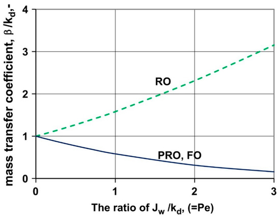
Figure 4.
The variation of the dimensionless mass transfer coefficient () according to the number (i.e., ). If the value of is kept constant, the value of increases in the RO process as the number increases. On the other hand, in the FO/PRO processes, the value of goes down while the number increases. In this figure, ; ; ; ; ; ; and . [50] The figure is reproduced from Reference [50] with permission.
2.3. Water Flux Models Applicable to PRO
2.3.1. Water Flux Models for Flat-Sheet Membrane
Since the first model of water flux—Equation (7)—was developed, many models describing the water flux in the PRO process appeared. The aforementioned water flux model developed by Lee et al. [37] is the first model that considered the impact of CP by taking the concentration of ICP into account. The water flux model developed by Lee et al. is given as
Equation (29) can be obtained by constructing a set of simultaneous equations with the relations used in solving the concentration of ICP, which are Equations (12)~(18), and by removing the salt flux terms in the resultant term. Although Equation (29) is the first equation providing insight into the impact of CP, it is not possible to find an analytical solution due to its non-linearity. Therefore, the iterative method based on a numerical analysis should be utilized for approximating the value of water flux. It should be noted that all water flux models hereafter, including the impacts of CP, are estimated with a numerical analysis. However, such numerical analysis methods are relatively difficult to apply because the approximation results can be uncertain along with given simulation conditions. Fortunately, a previous study demonstrated that the water flux models together with CPs can be converted into polynomial functions by Taylor expansion and it was found that the expanded polynomial functions can be used instead of the original water flux models to some extent [56].
After the development of Equation (29) in 1981, no additional water flux models were developed for several years. In 2009, a new water flux model which accounts for the impact of dilutive ECP was developed by Achilli et al. [29], as given below,
Subsequently, Yip et al. [57] developed a new water flux model simultaneously taking into consideration ICP, dilutive ECP, and the effect of salt flux on the region of dilutive ECP. That is, concentrative ECP on the feed side was not considered for this model. Therefore, and are denoted as the concentrations for the feed side and the draw side, respectively. By subtracting Equation (17) from (20), the following relationship is yielded:
Equation (31) represents the concentration difference between the draw side and the feed side in a system. By incorporating Equations (1), (7), and (31), the final form of Yip model is shown as follows:
Equation (32) might be the most widely utilized water flux model in the recent PRO-basis research. This model not only reflects the impact of ICP and dilutive ECP but also considers the mass balance of salts within the boundary layer region of dilutive ECP. Hence, almost every effect of salts on the given system can be considered with this model, with the exception of concentrative ECP. However, the impact of concentrative ECP is negligible compared to that of ICP [44], so it is generally not necessary to consider. Figure 5 displays the distinctions among Equations (7), (29), (30), and (32), which are made along with the types of CPs and factors considered by each model. As given in Figure 5a, the water flux declines as the number of factors considered for water flux models increases. The declined water flux eventually results in a decrease of , as shown in Figure 5b.
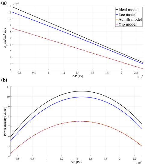
Figure 5.
The variation of the water flux () and power density according to the external hydraulic pressure (). As seen in (a), the water flux in a PRO process gradually decreases as the types of concentration polarization are taken into consideration. Consequently, the magnitudes of power density naturally decrease, as shown in (b). In these figures, ; ; ; ; ; ; and .
2.3.2. Water Flux Models for Hollow Fiber Membrane
The models described thus far are mainly applied to the flat-sheet membrane types. Because the geometries of membranes are different for each membrane configuration, it is necessary to find optimized models for each case. As widely known, the hollow fiber membrane configuration is a good alternative to the flat-sheet membrane type. Since the fundamental structure of the cross-section of a fiber in the hollow fiber membrane configuration is round in shape, Sivertsen et al. constructed a water flux relation for the hollow fiber membrane [58] as follows:
Here, and represent the distance from the center of a single fiber and the radius to the outer skin of a single fiber, respectively, and stands for the water flux at the outer skin of a single fiber. This relationship is based on the logic that the amount of water flux within and outside of a fiber cannot be equal due to the difference of membrane area (See the structure of hollow fiber membrane shown in Figure 6). Equation (13) becomes the following equation after Equation (33) is substituted for of (13):
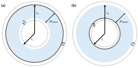
Figure 6.
The cross-sectional diagrams of a single hollow fiber of which a selective layer is positioned at (a) the outer skin, and (b) the lumen side.
To find the concentration difference between an outer-shell skin and inner porous layer (), Equation (34) should be integrated along with boundary conditions shown below:
Here, represents the concentration at the interfacial region between the porous layer and the outer-shell skin. Therefore, is the concentration difference between and (i.e., ). By incorporating the results obtained from integration steps, is finally given as,
Here, represents the thickness of a single fiber, as shown in Figure 6. By incorporating Equations (1), (7), and (36), the water flux model for a hollow fiber membrane can be obtained. Incidentally, note that Sivertsen et al. positioned the draw solution and the feed solution outside and inside of a hollow fiber membrane, respectively. This sort of solution positioning is the opposite of the conventional orientation for PRO: usually, the draw solution in a PRO system faces the active layer of a membrane. Therefore, the concentration distribution in Figure 6 does not hold for the Sivertsen model.
In another paper, Zhen Lei Cheng et al. [44] expanded the water flux models, based on the methodology of Sivertsen et al., for the hollow fiber membrane configuration (see Figure 6) as given in Equations (37a) and (37b),
Here, represents the radius to the inner skin (lumen) of a single fiber (Figure 6). Equations (37a) and (37b) represent the water flux models for cases in which a selective layer is located at the inner skin and the outer skin, respectively. The difference in the forms of Equations (37a) and (37b) reflects that the characteristic lengths of a hollow fiber configuration are the primary consideration. As the terms appear in both Equations (37a) and (37b), it could be concluded that plays a key role in calculating the water flux of a hollow fiber membrane configuration—clearly, . Therefore, the existence of a porous layer, which has been referred to as a support layer in this review, is of huge importance for a hollow fiber membrane. Equations (37a) and (37b) have a special meaning in that these relations, for the first time, describe the water flux of a hollow fiber membrane configuration by considering its signature design. One should note is that the water flux models for a hollow fiber configuration are not the irreplaceable ones since the water flux models for the flat-sheet membrane configuration are also applicable for the hollow fiber membrane configuration to some extent. However, the difference between the two types of models starts to appear as the scale of membrane configuration grows larger. In the aforementioned paper of Zhen et al., they demonstrated in their paper that the results of the hollow fiber models and the flat-sheet models are identical if ECP is assumed to be negligible [44]. However, they also showed that the impact of the difference in membrane designs should be taken into account, due to the increased ECP, as the size of the membrane configuration grows sufficiently large.
In this section, fundamental theories that have been researched with a stand-alone PRO configuration were introduced. The theories explained in this section will be used to describe the simulation and modeling works on an RO-PRO hybridized process in the subsequent section.
3. Hybridization of a PRO Process with RO
RO has played a significant role in relieving water stresses around the world. In spite of the considerable technological advancements in RO made in recent decades, however, this process is still considered energy-intensive. Toward the goal of reducing the energy consumption of RO while maintaining the same water productivity, a strategy to employ a PRO process in conjunction with RO is considered an effective approach. In this section, various types of modeling and simulation studies that sought to demonstrate the efficiency of an RO-PRO hybridized process will be introduced, and the possibility and the current limit of the corresponding process will be discussed.
3.1. Theoretical Energy Consumption in an RO Process
A PRO process is not commonly considered a type of desalination process. The seawater desalination process, which is mainly represented by the RO process, is literally a process of attracting seawater to produce clean freshwater by consuming energy. On the other hand, PRO is a process of which the main purpose is to produce energy, unlike the conventional seawater desalination processes. However, due to the similarity of the basic driving principle and the know-how accumulated over a long period of time, the analysis method of RO is usually applied to a number of PRO processes. Therefore, to understand the PRO process well, it is necessary to understand the basic principles of the RO process. Conversely, the principles of a PRO process can be applied to an RO process, as well.
Before considering the mathematical models of an RO-PRO hybridized process, it is worthwhile to investigate the energy consumption magnitude of an RO process because it has been researched even more widely than that of a PRO process. In addition, recognizing the magnitude of RO energy consumption may provide clues regarding the energy recovery efficiency of PRO to researchers.
The main interest of recent desalination processes including RO is to reduce the energy consumption as much as possible. Therefore, the minimum energy consumption calculated with thermodynamics plays an important role in setting an objective of a given desalination process. To discuss the minimum value of energy consumption required for the seawater desalination process, the theoretically ideal energy consumption is often referred to as the thermodynamically minimal energy (TME). For the RO process at 50% of the water recovery rate () and 35,000 ppm of the sodium chloride concentration in the feed solution, this value is calculated to be 1.1 kWh/m3: this value includes only RO train energy consumption and does not encompass the energy recovery device. A further widening of the investigation reveals that TME consumption is much lower for the entire desalination process. According to a previous study, the thermodynamic minimum energy required for the desalination process is estimated to be 0.7 kWh per cubic meter of permeate (i.e., 0.7 kWh/m3), when produced without an additional energy recovery [59].
Meanwhile, the actual energy consumed by current RO is today about 2 kWh/m3 at 50% of water recovery [60]. Considering the TME calculated for RO process (=1.1 kWh / m3), it is apparent that more work remains to be done. However, it should be noted that the TME of RO is actually impractical because it is the result of a batch RO process. In the case of the batch RO process, the concentrated brine discharged from the RO train is returned to the supply tank after the permeation step and the concentrated brine water is injected again into the RO train (Figure 7). This cycle continues until there is no more water to extract from the brine. Batch RO processes exhibit higher energy efficiency than semi-batch RO and multi-stage RO systems. This is because the batch RO results in the reduced entropy generation and thereby exhibits less entropic energy loss [61]. On the other hand, semi-batch RO and multistage RO systems are conventional process configurations used for reducing the energy consumption magnitude of a stand-alone RO process. However, the batch RO process cannot be applied in a real field because its water production rate is excessively slow. Therefore, the values of TME shown above should be regarded as ineffective ones in an actual RO process [61] unless accompanied by an innovative configuration for the batch RO process. This perspective underscores the utility of the PRO process in energy reduction in an actual RO process.
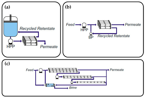
Figure 7.
The schematic illustrations of the configurations of each RO type: (a) batch-configuration, (b) semi-batch configuration, and (c) multistage configuration. In these figures, HPP stands for the high-pressure pump and BP stands for the brine pump [61]. The figure is reproduced from Reference [61] with permission.
3.2. An Ideal RO-PRO Hybridized Process: Thermodynamic Approaches
3.2.1. A Fundamental Relationship between the Pressure and Specific Energy
Investigating the relationship between the pressure and specific energy (SE) is worthwhile because the derivation steps of this relation comprise the theoretical background of membrane-based desalting processes. In membrane-based desalting processes, SE is defined as the energy per unit volume of permeate (kWh/m3). If the energy per unit volume of permeate is ‘consumed’ to produce freshwater, then SE is labeled the specific energy consumption (SEC). On the other hand, if the energy per unit volume of permeate is ‘recovered’ by the mixing process, SE turns into specific energy recovery (SER). That is, SEC and SER are energy units for the RO and PRO processes, respectively. Unlike the case of a stand-alone process, a PRO subunit process in an RO-PRO hybridized process must utilize a unit of SE because is incompatible with SEC. Considering that one of the objectives of a PRO subunit process in a hybridized RO-PRO is to reduce the energy consumption of RO, understanding the essence of SE is hugely important. To clarify the actions upon these terms, a dimension analysis procedure will be described hereafter. The SI unit of pressure is given as Pa, which is identical to [11,62]
where denotes newtons, the unit of force. Manipulating the right-side term slightly yields the following relation:
After offsetting in the numerator with in the denominator, the term turns into (watt) according to the definition. Since and , (39) is now rearranged as,
Thereby,
A final result shown in Equation (41) implies that the pressure itself in the membrane-based desalting processes can be converted to SE. Consequently, it can be concluded that the unit of SE is the same as that of the pressure for all the equations and relations regarding SE that will be mentioned subsequently, regardless of whether each pressure term represents the hydraulic pressure or the osmotic pressure. Equations from Equations (38) to (41) show that the energy efficiency of an RO-PRO hybridized process basically results from the ratio of net driving pressures in each membrane-based desalting process. To maximize the energy efficiency of an RO-PRO hybridized process, the optimization works for net driving pressure have to be accompanied. However, it is impractical to conduct the optimization works only with the rough results from Equations (38) to (41). In the next subsection, rigorous models established based on fundamental thermodynamics for RO and PRO processes will be addressed.
3.2.2. Thermodynamic Models for RO and PRO Processes
In this subsection, thermodynamic models for calculating the ideal energy consumption and energy recovery in the RO-PRO hybridized process are described. The first value to be calculated for the energy terms in the RO-PRO process is the thermodynamic work of each subunit process. The thermodynamic work () is defined as follows,
To derive the ideal energy consumption term of RO and the ideal energy recovery term of PRO, Equation (42) should be modified appropriately. The idea of derivation is based on the fact that can be expressed by the molar fraction of the lower-concentration solution () and the molar fraction of the higher-concentration solution () in a reversible membrane-based process [11,23,63,64,65,66,67]. This idea can be depicted as an imaginary reversible system comprised of two distinct solutions, positioned at the other sides of a membrane, with different concentrations. A depiction of such a system is given in Figure 8.
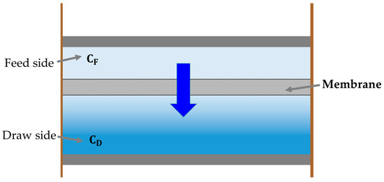
Figure 8.
The schematic illustration of a reversible membrane-based process. In accordance with the ideal assumptions, only water on a feed side permeates to a draw side through a membrane, and salts in the draw side do not transfer to the feed side.
In this system, for the sake of simplicity, the volume of each solution is assumed to be the same as the volume of the respective chambers, like a piston. If an arbitrary amount of water shifts from the less concentrated side to the more concentrated side, the mass balance of a complete system can be represented as below,
where stands for the volume of each solution, and subscripts , , , and stand for higher-concentration solution, lower-concentration solution, initial state, and shift, respectively. Then, the following relation appears if Equations (1), (43), and (44) are combined.
Equation (45) can be simplified as below if the concentration of a lower-concentration solution is negligible compared to that of a higher-concentration solution:
Now the ideal energy recovery term of PRO can be obtained as Eqations (42) and (46) are incorporated. Herein, is assumed to be equivalent to .
Equation (47) takes on a new form as it is rearranged appropriately with Equation (43):
Here, is the amount of ideal work per unit volume of the solution that shifted from the lower concentration side to the higher concentration side in a PRO process. Therefore, is SER. Above, Equation (48) represents the ideal energy recovery term of PRO process. Likewise, the ideal energy consumption term of RO process can be determined in a similar manner. The ideal energy consumption term of RO process is given as below,
Here, the subscript stands for the concentrated brine solution discharged from an RO process. If the RO and PRO processes are connected, the concentrated brine solution discharged from the RO subunit process serves as the draw solution in the PRO process. In that case, the signs of Equations (48) and (49) should be opposite to each other. For example, the sign of Equation (48) should be + if the sign of Equation (49) was designated as −, and vice versa.
From the derivations of Equations (48) and (49), it can be remarked that the ideal energy terms shown above are calculated only with the osmotic pressures of the lower-concentration solution and the higher-concentration solution of each subunit process. Those results hint at the role of a membrane only with a term —when it comes to an actual process, the membrane parameters become more important to estimate more precisely.
Equations (48) and (49) can also be derived by another approach of utilizing Gibbs free energy difference. The infinitesimal change of Gibbs free energy is generally defined as [67,68],
where , , and indicate the entropy of a system, chemical potential of component , and number of moles for component , respectively. For the mixing process of the less-concentrated solution and the more highly concentrated solution, it is assumed that there is no change in the temperature and pressure (i.e., ). Meanwhile, the chemical potential of an ideal solution is given as,
where represents the chemical potential under standard conditions and represents the mole fraction of component . Subsequently, according to the energy balance, a final form which is based on Equations (50) and (51) appears as follows [9,69,70,71],
where a subscript indicates the mixed solution. Herewith, all the assumptions used for Equations (43) and (44) should be utilized once again: that is, the concentration of the lower-concentration solution is negligible compared to that of the higher-concentration solution (i.e., ), and the total mass of a given system is conserved (i.e., ). Hence, the following relation is produced:
After a few steps, the final form of Equation (53) becomes identical to Equation (48). The existence of in Equation (53) results from the composition of NaCl in a solution, which dissolves into Na+ and Cl− in an aqueous state. In many previous studies [9,23,64,67,69], Gibbs free energy has been calculated without the presumption of the negligible low concentration of the lower-concentration solution. Without that presumption, Equation (53) becomes
Regardless of approaches for derivation, conclusions made so far imply the same lesson: no membrane parameters such as and are taken into consideration for computing the ideal energy recovery or consumption. However, the membrane parameters or the efficiencies of auxiliary instruments must be considered when calculating the energy recovery or consumption of actual processes since the water flux plays a critical role in tallying .
3.3. In the Case of an RO-PRO Hybridized Process
In a thermodynamic approach, it could be found that the theories for the RO and PRO processes coincide in many aspects. However, such common features are not valid for realistic RO and PRO processes. In this subsection, the methods of calculating the SEC of RO and SER of PRO processes are independently described, and the differences between the methods in tallying SE are discussed.
3.3.1. Specific Energy Consumption Model of RO Process with Process Efficiencies
The total energy efficiency of the RO-PRO hybrid process cannot be calculated with only Equations (48) and (49) if the efficiency of the pump, energy recovery device, and membrane is related to the actual operation of the process. The term “ideal” mentioned in a previous subsection indicates that all efficiencies within the process are 100%, but the process efficiency in the real world is never 100%. Therefore, in order to predict the energy efficiency of the process in accordance with the realistic constraints, all factors should be considered as much as possible. Zhu et al. derived a SEC model of real RO process () as follows [72,73],
where represents the efficiency of the high-pressure pump, and represents the efficiency of the energy recovery device, and indicates the rejection rate of an RO membrane. It should be noted that in Equation (55) stands for the feed solution in an RO process, not in a PRO process. Typically, is assumed to be in the range of approximately 0.8 to 0.85, and is assumed to be in the range of approximately 0.95 to 0.98 [28,69,74,75,76,77,78,79]. As shown in Figure 9, the SEC of a stand-alone RO process changes as and vary. In spite of this change, stand-alone RO processes, in particular a seawater RO process, conventionally set the water recovery rate as 0.5, considering the productivity of freshwater. However, such a conventional operational condition only holds for a stand-alone RO process. By contrast, in the case of an RO-PRO hybridized process, the energy efficiency becomes lowest at a water recovery rate of 0.5. This tendency of the RO-PRO hybridized process will be elaborated in a later subsection.
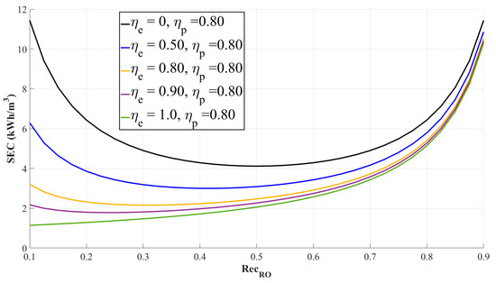
Figure 9.
The plot depicting the specific energy consumption (SEC) trend in a stand-alone RO process. As shown in the figure, a graph with the zero of energy recovery device efficiency () displays an almost perfectly symmetric parabola shape, and its specific energy consumption becomes lowest at 0.5 of the water recovery rate. Meanwhile, parabolic trends in other graph lines descend as the efficiency of an energy recovery device increases. In this figure, ; .
3.3.2. Dilutive Factor of the PRO Process
Once a PRO process is combined with an RO process, the energy consumed by the RO is automatically recovered to some extent by the PRO process. However, in order to maximize the energy recovery efficiency, it is necessary to consider not only the system parameters of RO such as but also the system parameters of PRO. One of the PRO system parameters that should be considered when operating the RO-PRO hybridized process is called the dilutive factor () and is defined as follows [25,80],
where represents the volumetric flow rate of the draw solution exiting the PRO process. As increases, the amount of energy that can be extracted from the PRO process increases. Interestingly, it was also found that increases along with (Figure 10). This is because a larger amount of water moves across the membrane as the concentration of the draw solution increases: recall that = . In the PRO process, the larger the amount of , the higher the energy generation; and more energy is extracted in the PRO process as increases. However, because the energy consumption of RO also increases along with , the absolute energy production of the PRO process itself is not highly significant in the overview of the RO-PRO hybridized process. The overall energy recovery efficiency of the RO-PRO process will be addressed in a later subsection, taking into account the respective effect of on the RO and PRO processes.
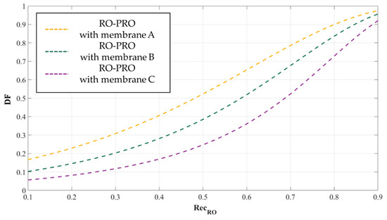
Figure 10.
The relationship between the water recovery rate () of an RO process and the dilutive factor () of a PRO process in an RO-PRO hybridized process. Dashed graph lines in this figure clearly show that the values of increase as becomes higher. In this figure, membrane performances: membrane A > membrane B > membrane C; and .
3.3.3. Specific Energy Recovery Models of the Module-Scale PRO System
As mentioned at the end of Section 3.3.1., it should be noted that the energy efficiency of an RO-PRO process with ideal conditions is not related to the operational constraints of a realistic process, but only to the concentration of the feed and draw solutions. If other operational constraints are added to a given process, the results vary significantly. To take the realistic operational constraints into consideration, imagine a PRO membrane module for which the process is subjected to constant external hydraulic pressure, and the draw and feed solutions flow counter-currently. Here, counter-current indicates a system configuration in which the draw and feed solutions of PRO are injected at opposite ends and directed to flow in the reverse direction: that is, a module inlet position for the draw solution becomes a module outlet position for the feed solution in the counter-current configuration, and vice versa. To calculate the maximum in the counter-current membrane module configuration, the following equation can be used [81,82,83,84]:
By contrast, the maximum with ideal conditions can be calculated as follows [71,85]:
Equation (58) is derived by differentiating Equation (54) with respect to . As seen in Figure 11, calculated from Equation (57) is always about 20~30% lower than the calculated from Equation (58). A discrepancy between Equations (57) and (58) is attributed to the nature of mass transport phenomena in a PRO process. When Equation (58) was derived, the salt flux heading for the feed side was overlooked according to the ideal assumptions. In addition, the mixing process between the feed and draw solutions was assumed to be perfect mixing, which never happens in an actual process due to the limitations of the membrane area. Considering that the membrane area is not a constituent used for calculating SEC of RO, a decisive difference in tallying the SE of RO and PRO processes can be discovered hereby [9,10,83]. Another piece of knowledge that can be obtained from the result of Figure 11 is the thermodynamic limits of the stand-alone PRO process. As shown in Figure 11, the maximal SER of the module-scale PRO process with 0.6 M NaCl o the draw solution and 0.015 M NaCl of the feed solution is around 0.26 kWh/m3 [12,84]. Here, 0.6 M NaCl represents the global average of seawater salinity. Considering that the energy consumption of the pretreatment facility for seawater desalination plants generally ranges from 0.24 to 0.40 kWh/m3 [86], such a magnitude of SER may not be even compatible with the pretreatment step for the stand-alone PRO process. Furthermore, the feed solution for the PRO-basis process also needs to be pretreated unless the feed solution is DI, so that the additional energy consumption is required for the PRO-basis processes. On the other hand, the energy efficiency of PRO increases as the process utilizes the brine from RO as the draw solution. After the stand-alone PRO process is hybridized with the seawater RO with 50% of the water recovery rate, the maximal SER leaps from 0.26 kWh/m3 to 0.55 kWh/m3 if the brine is selected as the draw solution [12]. Even though the value is still far less than the energy consumption magnitude of the RO plants, such a degree of energy recovery helps the energy consumption of the seawater desalination plant to be decreased, at least. This kind of thermodynamic limit of the stand-alone PRO process leads the trend of PRO-related studies to the PRO-hybridized processes.
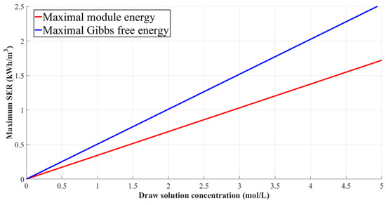
Figure 11.
The comparison of maximal specific energy extracted from the mixing process between the feed solution and the draw solution of a PRO process. The blue line indicates the maximal harvested under an ideal condition, . The red line indicates the maximal harvested under counter-current module conditions, . The figure was redrawn by the authors of the current review based on References [12,14].
The introduction of additional operational constraints to the PRO process, such as the actual high-pressure pump efficiency and membrane parameters, further reduces the inherent energy recovery of the PRO process. In such a general case, an optimized net external pressure () can be used to calculate the in the module scale PRO. refers to the hydraulic pressure reflecting all effects of concentration polarization and frictional loss on the PRO process. In this case, the of the PRO process at the module scale level can be generally explained as follows [65,85,87,88],
where is the sum of the volumetric flow rate of the permeate in a PRO subunit process, is the total membrane area, and is the average water flux of PRO. Since is defined as , all terms of the numerator and denominator can be offset except for . Therefore, Equation (59) can be expressed as the following equation:
models of the PRO process at the module scale are given by Equations (57) and (60), but there is a significant difference between these two equations. Equation (60) is affected by changes in membrane performance parameters such as , , and . Nevertheless, Equation (57) only varies according to changes in concentrations in a given process, even though the deployment of the feed and draw solutions and continuous mass transport phenomena were taken into consideration for a model.
3.3.4. Performance Indices for Evaluating a Complete RO-PRO Process
The method of calculating the energy efficiency of an entire RO-PRO process has been applied differently in each study, and as of yet there is no standardized method. This is partially because of the lack of a full-scale RO-PRO process. Nonetheless, some modeling and simulation studies have proposed methods to compute the energy efficiency of a complete hybridized process. In this subsection, a few such examples are presented.
Prante et al. proposed a formula for calculating the net energy consumption of RO-PRO as follows [65]:
With Equation (61), it is easy to see the net energy consumption resulting from the PRO subunit process in a complete hybridized process. Figure 12 represents the results of net specific energy sensitivity analysis in the RO-PRO hybridized process, calculated using 64 virtual membranes based on combinations of the main membrane parameters , , and . As expected, the results of the sensitivity analysis show that the net energy consumption of the RO-PRO hybridized process decreases as the value of increases and the values of and decrease.
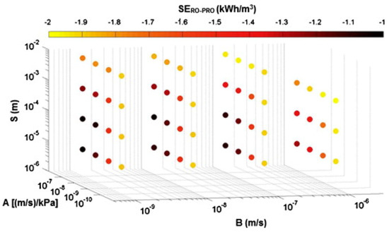
Figure 12.
The results of sensitivity analysis of an RO-PRO hybridized process using 64 virtual membranes. In this figure, , and [65]. The figure is reproduced from Reference [65] with permission.
In a different direction, Kim et al. [46,89] constructed an economic assessment index that converts the final products of the RO-PRO (i.e., water and electricity) into monetary benefits:
Here, and are the price of electricity and the price of water, respectively, for a given country or region; and are the energy produced by the PRO subunit process and the amount of work done by the pump, respectively. This index reflects that the products of each subunit process in an RO-PRO hybridized process are different from general electricity and freshwater characteristics.
In another study, a dimensionless performance index was used to observe the energy efficiency trend of the RO-PRO hybridized process [25]. The dimensionless performance index is given as follows,
where and represent the volumetric permeate flow rates of RO and PRO, respectively. The physical meaning of Equation (63) is the ratio of the energy recovered by the PRO subunit process to the total energy consumption in a complete RO-PRO hybridized process. A difference between Equation (63) and other performance indices is that Equation (63) can be applied to an RO-PRO process of any scale. The scale of the PRO subunit process should be smaller than that of the RO subunit process considering that the brine discharged from the RO process becomes the draw solution of the PRO process. In this context, Equation (63) aids in calculating the energy efficiency of a complete RO-PRO hybridized process as a reasonable comparison by removing the dimension of process sizes. As given in Figure 13a, the conventional water recovery rate of RO, which typically ranges from 0.4~0.6, is not effective if the energy efficiency of the RO-PRO hybridized process is calculated based on Equation (63). This is because a higher water recovery rate of the processes configured prior to PRO contributes to an increased energy consumption, while a higher concentration of brine resulting from the increased water recovery rate contributes to enhancing the energy recovery of the full hybridized process. Furthermore, since is also a function with respect to , the shape of the graph is changed as a domain is transformed from to . As shown in Figure 13b, a higher value of does not always guarantee a higher . In short, the decrease of in Figure 13b means that a higher permeate flow rate across a membrane is not always more energy-efficient for an RO-PRO hybridized process.
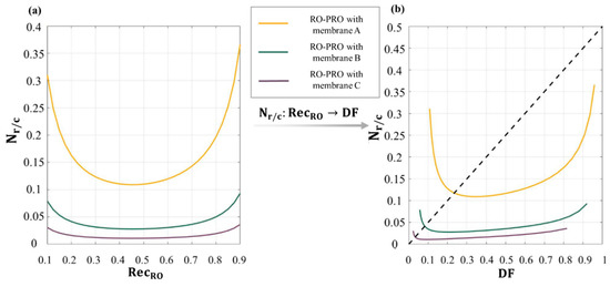
Figure 13.
The variation of the dimensionless performance index () for an RO-PRO hybridized process according to (a) the water recovery rate of RO (), and (b) the dilutive factor of PRO (). Since is a function with respect to , the trend of can be tracked along the change of . In this figure, membrane performances: membrane A > membrane B > membrane C; ; ; and [25].
Thus far, the results of numerous modeling and simulation studies have been described to explain the RO-PRO process. Thanks to those studies, the effectiveness of a PRO process to reduce the energy consumption of an RO process was demonstrated. Furthermore, the operational constraints that should be considered for running a process became even clearer due to a series of simulation studies. However, obstacles remain for implementing a full-scale RO-PRO process. In the last section, issues that hamper the commercialization of the RO-PRO hybridized process will be described, and tactics for overcoming those challenges will be explained in brief.
4. Major Challenges and Suggested Solutions for PRO-Basis Process
4.1. Major Challenges of PRO-Basis Process
4.1.1. Challenge 1: Choosing Membrane Configuration
PRO-process technology has already achieved a high level of power density at lab-scale studies. However, the amount of power density at that level has not yet been identified in the module-level PRO process. A total of 10~25 W/m2 of power density with a lab-scale PRO process [90,91] drops to 5 W/m2, or even to 1~2 W/m2 in a module scale [41,56,89,92,93]. Such a declination in the process performance can be attributed to the hindrance to water flux triggered by the increased thickness of the support layer of a spiral-wound membrane module. A conventional spiral-wound membrane module consists of several leaves, wherein the term leaf indicates a single sheet of flat-sheet membrane. Those multiple leaves are wound around a core bar of a module. Naturally, the thickness of the support layer increases as the scale of the module is enlarged. The increased thickness of the support layer thickness leads to an increase in the solute resistivity, : see Equation (18). The higher solute resistivity causes the water flux to decline since the increased makes a term increase and the increased results in the decline of water flux: see Equation (32). In addition to that hindrance, various modeling studies demonstrated that many factors contribute to the declination of water flux as the scale of a PRO process increases, while yielding lower values of power density than that of a lab-scale process [56,83,94]. The implication is that a fundamental improvement for the spiral-wound membrane module of a PRO process should be found to solve these scale-up problems.
On the other hand, a hollow fiber membrane module is free from the drawback of the spiral-wound type module. Unlike the spiral-wound module, the scale of the hollow fiber type module grows significantly as the number of fibers inside a module duct increases. Given that each fiber in the module acts independently, the thickness of the support layer of a hollow fiber type module is not worrisome. Moreover, it was already clarified that the energy productivity of a hollow fiber module is even higher than that of a spiral-wound module [95]. However, the hollow fiber module has a critical drawback in its robustness: since the thickness of a porous layer of a single fiber is relatively shorter than that of a flat-sheet membrane, the fiber is more prone to cracks if exposed to high external hydraulic pressure. Advances in membrane fabrication technology have reduced the frequency of fibers cracking, but it still occasionally occurs. Worse, once a fiber is cracked, it is difficult to locate the defect [96]. Since it is almost impossible to find a cracked fiber with the naked eye, an extra test is required to detect the broken fiber. Thus, unless extremely robust fibers are used on the module, a long-term operation with the hollow fiber module is impractical because the cracking of fibers remains a risk.
Thus, it seems clear that a novel type of membrane, which combines the robustness of the material of a spiral-wound module and the high productivity of the material of a hollow fiber module, is urgently needed if the PRO process is to leap from its current status to the next level.
4.1.2. Challenge 2: Difficulty in Controlling Fouling Propensity
The accumulation of unwanted foulants inside or on the membrane has been identified as one of the major challenges for the PRO process by many experimental studies [13,14,15,16,17,18,19]. The occurrence of membrane fouling is attributed to various causes such as the influent of colloidal particles; the deposition and adsorption of organic compounds; the crystallization of dissolved inorganic compounds; and the adhesion, accumulation, and interfusion of microorganisms [19,97,98,99,100,101,102,103]. As a result of the fouling propensities, many harmful influences such as cake-enhanced osmotic pressure [104,105] aggravate the performance of the PRO process. Common features of such membrane fouling propensities are randomness and uncontrollability. Randomness refers to the irregularity of the compositions of the foulants: that is, the share of foulants for a given intake fluid may alter according to the site of a process, seasonal variation, and precipitation. For example, the impact of biofouling caused by algae can be at its height during a hot season due to the prosperity of algae [106]. Uncontrollability refers to a characteristic of foulants that are difficult to remove or clean once settled on a membrane. In particular, biofouling on or inside a membrane is not only difficult to remove but difficult even to detect [62].
In the case of an RO-PRO hybridized process, the effects of fouling on a PRO subunit process are relieved to some extent due to a pretreatment step for the RO subunit process. However, a probability of fouling that can have an impact on a PRO membrane cannot be ignored because the PRO membrane is much more vulnerable to the foulants than is an RO membrane. Therefore, it is highly required to predict whether the foulants under a specific condition (e.g., seasonality, temperature, and the degree of CP) can affect to the PRO membrane severely or not. The clear conclusion is that computational modeling of fouling propensity is urgently needed, given that determining a membrane-cleaning period and taking precautions are critical for the optimal and economic operation of a process.
4.2. Suggested Solutions for the Challenges
4.2.1. Suggested Solution 1: Next-Generation Membranes
A challenge in fabricating a PRO membrane is to simultaneously satisfy a high water permeability and a great tensile strength, as noted in Section 4.1.1. To fabricate such a membrane, many bold research studies on the topic of a “state-of-art membrane” have been conducted [36,107,108,109,110,111,112,113,114]. Among the diversity of such studies, studies regarding aquaporin membranes and graphene membranes are attracting attention. The water permeability of these membranes is known to be two to three orders of magnitude higher than conventional membranes due to their outstanding membrane properties, as given in Figure 14 [114]. In particular, the selectivity of an aquaporin membrane is theoretically 100%, so salts cannot transfer through the membrane. Considering that the water permeability of the aquaporin membrane is superior to conventional membranes (Figure 14a) [115,116], the aquaporin membrane may be the first membrane capable of achieving the trade-off between the selectivity and permeability of a membrane. In addition, according to previous studies, some of these kinds of next-generation membranes are highly robust [117,118]. Although many other next-generation membranes still show the unstable robustness, the possibility of highly strong next-generation membranes was shown due to the abovementioned works. Therefore, PRO process technologies are likely to advance further if these next-generation membranes are availed.
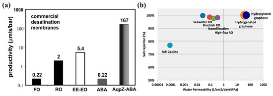
Figure 14.
A comparison of the water permeability of (a) an aquaporin membrane [115] and (b) a graphene membrane [114] to those of other commercial membranes. ‘Productivity’ on (a) is a unit which represents the same unit of ‘permeability’. In (a), EE-EO stands for a poly(ethylethylene)-poly(ethylene) oxide diblock polymer; ABA stands for a polymer vesicle without AqpZ; and AqpZ-ABA stands for a polymer vesicle with AqpZ. The figures are reproduced from References [114,115], respectively, with permission.
However, these next-generation membranes have various problems at present. Basically, such next-generation membranes are the byproducts of the combination of distinct fields: thus, the problems resulting from each field must be solved independently. For example, to fabricate an aquaporin membrane, protein structures embedded in a substrate should be economical and the combination of a membrane and the protein structures should not be intricate. Likewise, the combination of a membrane and graphene layers which accumulate on the membrane should be simple. Unfortunately, to satisfy all these requirements is not an easy task and requires a tremendous amount of experimental work [119]. Therefore, to achieve a higher reliability in the next-generation membranes more quickly, computational approaches that can simulate the passage of solvents through a membrane layer have been necessary. Molecular dynamics (MD) is one of the well-known computational approaches. MD is a computer simulation method to observe the interaction among atoms and molecules in a given time interval by constructing a virtual system [120,121]. In the virtual system, the classical mechanics and the statistical quantum mechanics are mainly applied to simulate the physical interactions of atoms and molecules [122]. In particular, MD has played a significant role in revealing not only how water molecules travel through the layers of next-generation membranes but also how efficiently salinity gradient desalting can perform with an aquaporin membrane and a graphene membrane [123,124]. Such excellence of MD was proved by previous studies. For example, MD can be employed to observe structures of the polyamide skin layer of an RO membrane [125]. In this research by Hirose et al., they showed that future attempts for developing high-performance composite RO membranes would include investigations about the molecular design of the cross-linked polyamide skin layers of membranes, entailing the use of molecular calculations and simulations. Another study [126] simulated the polymerization of a polyamide membrane from its corresponding monomers with MD. In the study, 250 monomers were prepared at the starting point and the polymerization procedure was shown graphically one by one as the merge of two types of monomers went on.
Considering that the scale of aquaporin channels and graphene layers is usually nano-size or smaller, it is highly challenging to produce next-generation membranes with the trial and errors of experimental works alone. Therefore, the importance of MD simulation must be emphasized above previous conventional membrane fabrication procedures.
4.2.2. Suggested Solution 2: Fouling Propensity Prediction Using Machine Learning and Computational Algorithms
A basic approach to control the fouling propensity on a membrane is to apply a feedback control principle to a process. With the feedback control principle, the operators of a process can detect the accumulation of foulants on a membrane by the declination of water flux or the increase of transmembrane pressure. The implementation of feedback control in a plant is based on the assumption that all states are available for online measurement. However, that assumption is impractical because some of the states may not be measurable due to a lack of appropriate devices or to the high price of sensors [127,128,129,130,131]. Furthermore, sensing the influent of foulants is an indirect method, such that proper actions against the foulants may come too late. A conventional method to take proactive actions against the fouling on a membrane without online measurement is to utilize the deterministic models which are derived from the water flux models represented in Section 2 [132]. With the deterministic fouling prediction models, the overall tendency of decline in water permeability according to the elapse of time can be generally tracked [133]. A point that the calculations required for the prediction are relatively simple is another advantage of such models. However, such kinds of deterministic fouling models cannot reflect the anomaly of fouling propensity since the equations of the deterministic models generally does not take the randomness factors into account [132,133]. To compensate for this problem, various types of machine-learning techniques and computer algorithms have been harnessed to provide a warning about the influent of foulants to the operator of a process with the reflection of fluctuation of the fouling propensity. Here, machine-learning techniques indicate the computational techniques based on the statistical learning process, which are widely used to classify, regress, and cluster the given datasets [134]. Generally, the machine learning steps are divided into three sessions, as below:
- Parameter (hyperparameter) setting.Parameters such as learning rate, number of hidden neurons, and the weights and bias of activation function are determined. The selected parameters contribute to the performance of modeling.
- Training session.In the training session, the partial fraction of total datasets are literally trained to fit a machine learning model into specific datasets. The fraction of a dataset used for this training session is quite variant, but usually more or less than 70% of the total datasets.
- Validation session.In the validation session, a model trained during the training session is validated with the rest of the datasets. With the result of the validation session, the overall performance of the machine learning model is assessed.
By applying the machine learning techniques, it is possible to predict the fouling propensity of a membrane, as well. For better comprehension, the prediction results of membrane fouling on an actual RO process are introduced in this subsection as an example [135,136,137]. As shown in Figure 15, various machine-learning-based models can be utilized to predict and diagnose the state of fouling. Out of many kinds of machine-learning techniques, representative examples include the artificial neural network (ANN), and the support vector machine (SVM) [134,138]. According to the model running results, the prediction accuracy of the ANN model is almost identical to that of the SVM model. In short, both models show a sufficient performance to predict the trend of membrane fouling. However, noise in between the result graph lines contributes to increased uncertainty in such models. To decrease the uncertainty of models, the Kalman filter is utilized to increase the prediction accuracy by reducing sensor noise (Figure 15c,d) [139]. When harnessing this Kalman filter technique, computational algorithms were designed to estimate and predict the unmeasured state of a process, which is caused by the lack of appropriate estimating devices [131]. A series of these results, which result from the incorporation of machine-learning techniques and the Kalman filter, imply that a high-quality prediction is available even without expensive devices. The biggest strength of machine-learning techniques is by far the availability of time-dependent analysis. Since these machine-learning techniques are based on stochastic methods, the random fouling propensities on a membrane can be tracked easily at any time and place.
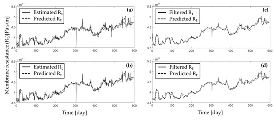
Figure 15.
The results of fouling prediction run by machine-learning-based techniques, with (a,b) showing results from the artificial neural network (ANN) and support vector machine (SVM) models, respectively, and (c,d) showing the application of a Kalman filter to reduce noise [135]. The figures were reproduced from Reference [135] with permission.
However, in spite of the excellence of machine-learning techniques, such stochastic methods are not versatile. To assure the high-quality performance of machine-learning models, sufficient amounts of datasets must be prepared; otherwise, the machine-learning models become incompetent in detecting the detailed fluctuations of the membrane fouling which take place in between the prediction duration. In other words, a preliminary data acquisition session should be guaranteed to enhance the performance of the machine-learning models. To be certain, the accuracy of the machine-learning models in the data acquisition session is relatively low. To accelerate data acquisition, various new means are being developed vigorously. Other than ANN and SVM, advanced machine-learning techniques such as the recurrent neural network are being studied further [140]. Moreover, the scope of machine-learning research for membrane fouling prediction can be expanded even to the boundary of deep learning. Thus, machine-learning-based techniques are expected to be used not only for predicting the fouling on a membrane, but also for imparting the real-time information regarding the membrane fouling in the future.
5. Conclusions
In this review, the authors reviewed many relevant studies which were directly or indirectly related to the simulation and modeling research of pressure-retarded osmosis (PRO) processes. The contents of those research papers were reorganized to enable better understanding by readers. Accordingly, the reorganized contents were divided into three parts as follows:
- The first part (Section 2. Fundamental theories of a PRO process) of the current paper was dedicated to describing the fundamental mathematical theories which are indispensable to understanding the mechanism of PRO. In the first part, the water flux models for the salinity gradient desalting processes were mathematically derived by combining the models with concentration polarization phenomena, and the derived water flux models were used for calculating the power density of a PRO process. The roles of the membrane parameters such as water permeability, salt permeability, and structural parameters were described according to the definitions and the physical implications of those parameters.
- In the second part (Section 3. Hybridization of a PRO process with RO), the hybridization features of an RO-PRO process and the inherent limit of a stand-alone PRO process were analyzed based on thermodynamic theories and the advanced theories of a PRO process resulting from the contents of Section 2. In this part, methodologies to calculate the energy efficiency of an RO-PRO hybridized process were mainly described with a thermodynamic concept called specific energy. With the specific energy concept, many models evaluating the energy efficiency of the RO-PRO process were developed. In this review, a few such RO-PRO energy efficiency models were introduced representatively.
- The last part (Section 4. Major challenges and suggested solutions for PRO-basis process) diagnosed the critical problems facing current PRO-basis processes, namely the membrane configuration of a stand-alone PRO process and the vulnerability of membranes to fouling. Novel approaches to overcome the aforementioned problems were discussed. Next-generation membranes such as aquaporin and graphene were suggested as potential breakthroughs to the membrane configuration challenge. Molecular dynamic simulation was suggested as a means to enhance the efficiency of next-generation membranes. In response to the propensity for membrane fouling, machine learning and computational algorithm methods were highlighted as effective alternative to make rapid progress.
Chronologically, the contents in each section of this review paper can be regarded as the past (Section 2), present (Section 3), and future (Section 4) of PRO-basis processes. As suggested in Section 4, the technological progress of the PRO-basis processes might not be made solely on the basis of the PRO technologies of the past. To maximize the performance of the PRO-basis processes effectively, a research scope of modeling and simulation studies should be widened beyond conventional process engineering. With this perspective, the authors strongly believe that this review can serve as a valuable resource providing a broad overview of the modeling and simulation studies of PRO-basis processes.
Funding
This research was supported by a grant funded by the Ministry of Land, Infrastructure and Transport (MOLIT) and Korea Agency for Infrastructure Technology Advancement (KAIA), grant number 16FIP-B116951-01).
Conflicts of Interest
The authors declare no conflict of interest.
References
- United Nations Framework Convention on Climate Change (UNFCCC). Adoption of the Paris Agreement. Available online: https://unfccc.int/resource/docs/2015/cop21/eng/l09r01.pdf (accessed on 12 January 2019).
- UNFCCC. Progress Tracker: Work Programme Resulting from the Relevant Requests Contained in Decision 1/CP.21. 2017. Available online: https://unfccc.int/sites/default/files/resource/pa_progress_tracker_200617.pdf (accessed on 12 January 2019).
- Yip, N.Y.; Vermaas, D.A.; Nijmeijer, K.; Elimelech, M. Thermodynamic, energy efficiency, and power density analysis of reverse electrodialysis power generation with natural salinity gradients. Environ. Sci. Technol. 2014, 48, 4925–4936. [Google Scholar] [CrossRef] [PubMed]
- Statkraft. Available online: https://www.statkraft.com/media/press-releases/Press-releases-archive/2007/statkraft-to-build-worlds-firsk-osmotic-power-plant/ (accessed on 12 January 2019).
- Skilhagen, S.E.; Dugstad, J.E.; Aaberg, R.J. Osmotic power-power production based on the osmotic pressure difference between waters with varying salt gradients. Desalination 2008, 220, 476–482. [Google Scholar] [CrossRef]
- Kim, J.; Kim, S.H.; Kim, J.H. Pressure retarded osmosis process: Current status and future. J. Korean Soc. Environ. Eng. 2014, 36, 791–802. [Google Scholar] [CrossRef]
- Saito, K.; Irie, M.; Zaitsu, S.; Sakai, H.; Hayashi, H.; Tanioka, A. Power generation with salinity gradient by pressure retarded osmosis using concentrated brine from SWRO system and treated sewage as pure water. Desalin. Water Treat. 2012, 41, 114–121. [Google Scholar] [CrossRef]
- Kurihara, M. Mega-Ton Water System including PRO. In Proceedings of the 1st International Symposium Innovative Desalination Technologies with INES Meeting, Seoul, Republic of Korea, 2 September 2014; pp. 217–223. [Google Scholar]
- Lin, S.; Straub, A.P.; Elimelech, M. Thermodynamic limits of extractable energy by pressure retarded osmosis. Energy Environ. Sci. 2014, 7, 2706–2714. [Google Scholar] [CrossRef]
- Banchik, L.C.; Sharqawy, M.H.; Lienhard V, J.H. Limits of power production due to finite membrane area in pressure retarded osmosis. J. Membr. Sci. 2014, 468, 81–89. [Google Scholar] [CrossRef]
- Reimund, K.K.; McCutcheon, J.R.; Wilson, A.D. Thermodynamic analysis of energy density in pressure retarded osmosis: The impact of solution volumes and costs. J. Membr. Sci. 2015, 487, 240–248. [Google Scholar] [CrossRef]
- Straub, A.P.; Deshmukh, A.; Elimelech, M. Pressure-retarded osmosis for power generation from salinity gradients: Is it viable? Energy Environ. Sci. 2016, 9, 31–48. [Google Scholar] [CrossRef]
- Honda, R.; Rukapan, W.; Komura, H.; Teraoka, Y.; Noguchi, M.; Hoek, E.M. Effects of membrane orientation on fouling characteristics of forward osmosis membrane in concentration of microalgae culture. Bioresour. Technol. 2015, 197, 429–433. [Google Scholar] [CrossRef]
- Touati, K.; Tadeo, F.; Chae, S.H.; Kim, J.H.; Silva, O.A. Pressure Retarded Osmosis: Renewable Energy Generation and Recovery, 1st ed.; Academic Press: Cambridge, MA, USA, 2018. [Google Scholar]
- Yip, N.Y.; Brogioli, D.; Hamelers, H.V.M.; Nijmeijer, K. Salinity gradients for sustainable energy: Primer, progress, and prospects. Environ. Sci. Technol. 2016, 50, 12072–12094. [Google Scholar] [CrossRef]
- Thelin, W.R.; Sivertsen, E.; Holt, T.; Brekke, G. Natural organic matter fouling in pressure retarded osmosis. J. Membr. Sci. 2013, 438, 46–56. [Google Scholar] [CrossRef]
- Yip, N.Y.; Elimelech, M. Influence of natural organic matter fouling and osmotic backwash on pressure retarded osmosis energy production from natural salinity gradients. Environ. Sci. Technol. 2013, 12607–12616. [Google Scholar] [CrossRef] [PubMed]
- Choi, Y.; Vigneswaran, S.; Lee, S. Evaluation of fouling potential and power density in pressure retarded osmosis (PRO) by fouling index. Desalination 2016, 389, 215–223. [Google Scholar] [CrossRef]
- Kim, J.; Park, M.J.; Park, M.; Shon, H.K.; Kim, S.H.; Kim, J.H. Influence of colloidal fouling on pressure retarded osmosis. Desalination 2016, 389, 207–214. [Google Scholar] [CrossRef]
- Touati, K.; de la Calle, A.; Tadeo, F.; Roca, L.; Schiestel, T.; Alarcón-Padilla, D.-C. Energy Recovery Using Salinity Differences in a Multi-Effect Distillation System. Desalination and Water Treatment 2014. [Google Scholar] [CrossRef]
- Touati, K.; Tadeo, F. INTEGRATION OF POWER RETARDED OSMOSIS IN SOLAR MULTIEFFECT DESTILLATION. In Proceedings of the 7th International Symposium on Design, Operation and Control of Chemical Processes (PSE ASIA 2016), Tokyo, Japan, 24–27 July 2016. [Google Scholar]
- He, W.; Wang, Y.; Shaheed, M.H. Enhanced energy generation and membrane performance by two-stage pressure retarded osmosis (PRO). Desalination 2015, 359, 186–199. [Google Scholar] [CrossRef]
- He, W.; Wang, Y.; Shaheed, M.H. Energy and thermodynamic analysis of power generation using a natural salinity gradient based pressure retarded osmosis process. Desalination 2014, 350, 86–94. [Google Scholar] [CrossRef]
- Kim, J.; Park, M.J.; Park, M.; Shon, H.K.; Kim, J.H. Performance analysis of reverse osmosis, membrane distillation, and pressure-retarded osmosis hybrid processes. Desalination 2016, 380, 85–92. [Google Scholar] [CrossRef]
- Chae, S.H.; Seo, J.W.; Kim, J.; Kim, Y.M.; Kim, J.H. A simulation study with a new performance index for pressure-retarded osmosis processes hybridized with seawater reverse osmosis and membrane distillation. Desalination 2018, 444, 118–128. [Google Scholar] [CrossRef]
- Lonsdale, H.; Merten, U.; Riley, R. Transport properties of cellulose acetate osmotic membranes. J. Appl. Polym. Sci. 1965, 9, 1341–1362. [Google Scholar] [CrossRef]
- Madsen, H.T.; Nissen, S.S.; Muff, J.; Søgaard, E.G. Pressure retarded osmosis from hypersaline solutions: investigating commercial FO membranes at high pressures. Desalination 2017, 420, 183–190. [Google Scholar] [CrossRef]
- Fritzmann, C.; Löwenberg, J.; Wintgens, T.; Melin, T. State-of-the-art of reverse osmosis desalination. Desalination 2007, 216, 1–76. [Google Scholar] [CrossRef]
- Achilli, A.; Cath, T.Y.; Childress, A.E. Power generation with pressure retarded osmosis: an experimental and theoretical investigation. J. Membr. Sci. 2009, 343, 42–52. [Google Scholar] [CrossRef]
- Achilli, A.; Childress, A.E. Pressure retarded osmosis: from the vision of Sidney Loeb to the first prototype installation – Review. Desalination 2010, 261, 205–211. [Google Scholar] [CrossRef]
- Kim, D.I.; Kim, J.; Hong, S. Changing membrane orientation in pressure retarded osmosis for sustainable power generation with low fouling. Desalination 2016, 389, 197–206. [Google Scholar] [CrossRef]
- Gray, G.T.; McCutcheon, J.R.; Elimelech, M. Internal concentration polarization in forward osmosis: role of membrane orientation. Desalination 2006, 197, 1–8. [Google Scholar] [CrossRef]
- McCutcheon, J.R.; Elimelech, M. Influence of concentrative and dilutive internal concentration polarization on flux behavior in forward osmosis. Desalination 2006, 284, 237–247. [Google Scholar] [CrossRef]
- Kim, D.I.; Kim, J.; Shon, H.K.; Hong, S. Pressure retarded osmosis (PRO) for integrating seawater desalination and wastewater reclamation: energy consumption and fouling. J. Membr. Sci. 2015, 483, 34–41. [Google Scholar] [CrossRef]
- Wong, M.C.; Martinez, K.; Ramon, G.Z.; Hoek, E.M.V. Impacts of operating conditions and solution chemistry on osmotic membrane and performance. Desalination 2012, 287, 340–349. [Google Scholar] [CrossRef]
- Park, H.B.; Kamcev, J.; Robeson, L.M.; Elimelech, M.; Freeman, B.D. Maximizing the right stuff: the trade-off between membrane permeability and selectivity. Science 2017, 356, 1137–1148. [Google Scholar] [CrossRef]
- Lee, K.; Baker, R.; Lonsdale, H. Membranes for power generation by pressure-retarded osmosis. J. Membr. Sci. 1981, 8, 141–171. [Google Scholar] [CrossRef]
- Touati, K.; Hänel, C.; Tadeo, F.; Schiestel, T. Effect of the feed and draw solution temperatures on PRO performance: theoretical and experimental study. Desalination 2015, 365, 182–195. [Google Scholar] [CrossRef]
- Thorsen, T.; Holt, T. The potential for power production from salinity gradients by pressure retarded osmosis. J. Membr. Sci. 2009, 335, 103–110. [Google Scholar] [CrossRef]
- Achilli, A.; Cath, T.Y.; Childress, A.E. Selection of inorganic-based draw solutions for forward osmosis applications. J. Membr. Sci. 2010, 364, 233–241. [Google Scholar] [CrossRef]
- Bui, N.N.; Arena, J.T.; McCutcheon, J.R. Proper accounting of mass transfer resistances in forward osmosis: improving the accuracy of model predictions of structural parameter. J. Membr. Sci. 2015, 492, 289–302. [Google Scholar] [CrossRef]
- Brouwers, H.J.H. Stagnant film model for effect of diffusional layer thickness on heat transfer and exerted friction. AlChE Journal 1995, 41, 1821–1825. [Google Scholar] [CrossRef]
- Miranda, J.M.; Campos, J.B.L.M. Mass transfer in the vicinity of a separation membrane – the applicability of the stagnant film theory. J. Membr. Sci. 2002, 537, 137–150. [Google Scholar] [CrossRef]
- Cheng, Z.L.; Chung, T.S. Mass transport of various membrane configurations in pressure-retarded osmosis (PRO). J. Membr. Sci. 2017, 537, 160–176. [Google Scholar] [CrossRef]
- Zydney, A.L. Stagnant film model for concentration polarization in membrane systems. J. Membr. Sci. 1997, 130, 275–281. [Google Scholar] [CrossRef]
- Kim, J.; Park, M.; Snyder, S.A.; Kim, J.H. Reverse osmosis (RO) and pressure retarded osmosis (PRO) hybrid processes: model-based scenario study. Desalination 2013, 322, 121–130. [Google Scholar] [CrossRef]
- Gekas, V.; Hallström, B. Mass transfer in the membrane concentration polarization layer under turbulent cross flow: I. critical literature review and adaptation of existing Sherwood correlations to membrane operations. J. Membr. Sci. 1987, 30, 153–170. [Google Scholar] [CrossRef]
- Bird, R.B.; Stewart, W.E.; Lightfoot, E.N. Transport Phenomena, 2nd ed.; John Wiley & Sons: Hoboken, NJ, USA, 2006; pp. 40–74. [Google Scholar]
- Phillip, W.A.; Yong, J.S.; Elimelech, M. Reverse draw solute permeation in forward osmosis: Modeling and experiments. Environ. Sci. Technol. 2010, 44, 5170–5176. [Google Scholar] [CrossRef] [PubMed]
- Nagy, E. A general, resistance-in-series, salt-and water flux models for forward osmosis and pressure-retarded osmosis for energy generation. J. Membr. Sci. 2014, 460, 71–81. [Google Scholar] [CrossRef]
- Koutsou, C.P.; Yiantsios, S.G.; Karabelas, A.G. Direct numerical simulation of flow in spacer-filled channels: Effect of spacer geometrical characteristics. J. Membr. Sci. 2007, 291, 53–69. [Google Scholar] [CrossRef]
- Koutsou, C.P.; Yiantsios, S.G.; Karabelas, A.J. A numerical and experimental study of mass transfer in spacer-filled channels: Effects of spacer geometrical characteristics and Schmidt number. J. Membr. Sci. 2009, 326, 234–251. [Google Scholar] [CrossRef]
- Li, F.; Meindersma, W.; de Haan, A.B.; Reith, T. Novel spacers for mass transfer enhancement in membrane separations. J. Membr. Sci. 2005, 253, 1–12. [Google Scholar] [CrossRef]
- Brian, P. Mass transport in reverse osmosis. In Desalination by Reverse Osmosis, 4th ed.; Merten, U., Ed.; MIT Press: Cambridge, MA, USA, 1966. [Google Scholar]
- Michaels, A.S. New separation technique for the CPI. Chem. Eng. Prog. 1968, 64, 31–43. [Google Scholar]
- He, W.; Wang, Y.; Shaheed, M.H. Modelling of osmotic energy from natural salt gradients due to pressure retarded osmosis: effects of detrimental factors and flow schemes. J. Membr. Sci. 2014, 471, 247–257. [Google Scholar] [CrossRef]
- Yip, N.Y.; Tiraferri, A.; Phillip, W.A.; Schiffman, J.D.; Hoover, L.A.; Chang Kim, Y.; Elimelech, M. Thin-film composite pressure retarded osmosis membranes for sustainable power generation from salinity gradients. Environ. Sci. Technol. 2011, 45, 4360–4369. [Google Scholar] [CrossRef]
- Sivertsen, E.H.; Thelin, T.W.; Brekke, G. Modeling mass transport in hollow fiber membranes used for pressure retarded osmosis. J. Membr. Sci. 2012, 417–418, 69–79. [Google Scholar]
- Shannon, M.A. Science and technology for water purification in the coming decades. Nature 2008, 452, 301–310. [Google Scholar] [CrossRef] [PubMed]
- Phillip, W.A.; Elimelech, M. The future of seawater desalination: energy, technology, and the environment. Science 2011, 333, 712–717. [Google Scholar]
- Werber, J.R.; Deshmukh, A.; Elimelech, M. Can batch or semi-batch processes save energy in reverse-osmosis desalination? Desalination 2017, 402, 109–122. [Google Scholar] [CrossRef]
- Wilf, M.; Awerbuch, L.; Bartels, C.; Mickley, M.; Pearce, G.; Voutchkov, N. The Guidebook to Membrane Desalination Technology: Reverse Osmosis, Nanofiltration and Hybrid Systems: Process, Design, Applications and Economics, 1st ed.; Balaban Desalination Publications: Rome, Italy, 2007. [Google Scholar]
- Spiegler, K.S.; El-Sayed, Y.M. The energetics of desalination processes. Desalination 2001, 134, 109–128. [Google Scholar] [CrossRef]
- Wang, Z.; Hou, D.; Lin, S. Gross vs. net energy: towards a rational framework for assessing the practical viability of pressure retarded osmosis. J. Membr. Sci. 2016, 503, 132–147. [Google Scholar] [CrossRef]
- Prante, J.L.; Ruskowitz, J.A.; Childress, A.E.; Achilli, A. RO-PRO desalination: an integrated low-energy approach to seawater desalination. Appl. Energy 2014, 120, 104–114. [Google Scholar] [CrossRef]
- Zhang, H.; Yang, W.; Rainwater, K.; Song, L. Limiting extractable energy from pressure-retarded osmosis with different pretreatment costs for feed and draw solutions. J. Membr. Sci. 2017, 544, 208–212. [Google Scholar] [CrossRef]
- Smith, J.M.; Van Ness, H.C.; Abbott, M.M. Introduction to Chemical Engineering Thermodynamics, 7th ed.; McGraw Hill: New York, NY, USA, 2004. [Google Scholar]
- Perrot, P. A to Z of Thermodynamics, 1st ed.; Oxford University Press: Oxford, England, UK, 1998. [Google Scholar]
- Post, J.W.; Veerman, J.; Hamelers, H.V.M.; Euverink, G.J.W.; Metz, S.J.; Nymeijer, K.; Buisman, C.J.N. Salinity-gradient power: evaluation of pressure-retarded osmosis and reverse electrodialysis. J. Membr. Sci. 2007, 288, 218–230. [Google Scholar] [CrossRef]
- Veerman, J. Reverse Electro-dialysis: Design and Experimentation by Modeling and Experimentation. Ph.D. Thesis, Rijksuniversiteit Groningen, Groningen, The Netherlands, 2010. [Google Scholar]
- Post, J.W.; Hamelers, H.V.M.; Buisman, C.J.N. Energy recovery from controlled mixing salt and fresh water with a reverse electrodialysis system. Environ. Sci. Technol. 2008, 42, 5785–5790. [Google Scholar] [CrossRef]
- Zhu, A.; Christofides, P.D.; Cohen, Y. On RO membrane and energy costs and associated incentives for future enhancement of membrane permeability. J. Membr. Sci. 2009, 344, 1–5. [Google Scholar] [CrossRef]
- Zhu, A.; Christofides, P.D.; Cohen, Y. Minimization of energy consumption for a two-pass membrane desalination: effect of energy recovery, membrane rejection and retentate recycling. J. Membr. Sci. 2009, 339, 126–137. [Google Scholar] [CrossRef]
- Stover, R.L. Energy Recovery Device Performance Analysis. In Proceedings of the Water Middle East Conference, Manama, Bahrain, 19–23 November 2005. [Google Scholar]
- Energy Recovery, Inc. Available online: www.energyrecovery.com/water/px-pressure-exchanger (accessed on 12 January 2019).
- Ye, X.Y.; Yang, S.S.; Hu, J.N.; Xiao, X.P.; Zhou, G.F. Research on Improving Efficiency of High Pressure Pump in Seawater Reverse Osmosis Desalination. In Proceedings of the ASME 2009 Fluids Engineering Division Summer Meeting, Vail, CO, USA, 2–6 August 2009; Volume 1: Symposia, Parts A, B and C. [Google Scholar]
- Papa, F.; Radulj, D. Thermodynamic method used for pump performance and efficiency testing program. Environ. Sci. Eng. Mag. 2013, 26, 44–48. [Google Scholar]
- Greenlee, L.F.; Lawler, D.F.; Freeman, B.D.; Marrot, B.; Moulin, P. Reverse osmosis desalination: water sources, technology, and today’s challenges. Water Res. 2009, 43, 2317–2348. [Google Scholar] [CrossRef] [PubMed]
- Stover, R.L. Seawater reverse osmosis with isobaric energy recovery devices. Desalination 2007, 203, 168–175. [Google Scholar] [CrossRef]
- Wan, C.F.; Chung, T.S. Energy recovery by pressure retarded osmosis (PRO) in SWRO-PRO integrated processes. Appl. Energy 2016, 162, 687–698. [Google Scholar] [CrossRef]
- Weinstein, J.N.; Leitz, F.B. Electric power from differences in salinity: the dialytic battery. Science 1976, 191, 557–559. [Google Scholar] [CrossRef] [PubMed]
- Wilson, A.D.; Stewart, F.F. Deriving osmotic pressures of draw solutes used in osmotically driven membrane processes. J. Membr. Sci. 2013, 431, 205–211. [Google Scholar] [CrossRef]
- Yang, W.; Song, L.; Zhao, J.; Chen, Y.; Hu, B. Numerical analysis of performance of ideal counter-current flow pressure retarded osmosis. Desalination 2018, 433, 41–47. [Google Scholar] [CrossRef]
- Straub, A.P.; Lin, S.; Elimelech, M. Module-scale analysis of pressure retarded osmosis: performance limitations and implications for full-scale operation. Environ. Sci. Technol. 2014, 48, 12435–12444. [Google Scholar] [CrossRef] [PubMed]
- Yip, N.Y.; Elimelech, M. Thermodynamic and energy efficiency analysis of power generation from natural salinity gradients by pressure retarded osmosis. Environ. Sci. Technol. 2012, 46, 5230–5239. [Google Scholar] [CrossRef]
- Seawater Desalination Power Consumption—White Paper; Watereuse: Alexandria, VA, USA, November 2011.
- Schock, G.; Miguel, A. Mass transfer and pressure loss in spiral wound modules. Desalination 1987, 64, 339–352. [Google Scholar] [CrossRef]
- Helfer, F.; Lemckert, C.; Anissimov, Y.G. Osmotic power with pressure retarded osmosis: Theory, performance and trends—A review. J. Membr. Sci. 2014, 453, 333–358. [Google Scholar] [CrossRef]
- Kim, J.; Jeong, K.; Park, M.J.; Shon, H.K.; Kim, J.H. Recent advances in osmotic energy generation via pressure-retarded osmosis (PRO): A review. Energies 2015, 8, 11821–11845. [Google Scholar] [CrossRef]
- Zhang, S.; Sukitpaneenit, P.; Chung, T. Design of robust hollow fiber membranes with high power density for osmotic energy production. Chem. Eng. J. 2014, 241, 457–465. [Google Scholar] [CrossRef]
- Song, X.; Liu, Z.; Sun, D.D. Energy recovery from concentrated seawater brine by thin-film nanofiber composite pressure retarded osmosis membranes with high power density. Energy Environ. Sci. 2013, 6, 1199–1210. [Google Scholar] [CrossRef]
- Atarde, D.; Jain, M.; Gupta, S.K. Modeling of a forward osmosis and a pressure-retarded osmosis spiral wound module using the Spiegler-Kedem model and experimental validation. Sep. Purif. Technol. 2016, 164, 182–197. [Google Scholar] [CrossRef]
- Hong, S.S.; Ryoo, W.; Chun, M.S.; Lee, S.O.; Chung, G.Y. Numerical studies on the pressure-retarded osmosis (PRO) system with the spiral wound module for power generation. Desalination & Water Treatment 2013, 52, 6333–6341. [Google Scholar]
- Chae, S.H.; Kim, J.H. Recent issues relative to a low salinity pressure-retarded osmosis process and suggested technical solutions. In Membrane-Based Salinity Gradient Processes for Water Treatment and Power Generation, 1st ed.; Elsevier: New York, NY, USA, 2018; pp. 273–295. [Google Scholar]
- Kurihara, M.; Takeuchi, H. SWRO-PRO system in “Mega-ton Water System” for energy reduction and low environmental impact. Water 2018, 10, 48. [Google Scholar] [CrossRef]
- Wan, C.F.; Li, B.; Yang, T.; Chung, T.S. Design and fabrication of inner-selective thin-film composite (TFC) hollow fiber modules for pressure retarded osmosis (PRO). Sep. Purif. Technol. 2017, 172, 32–42. [Google Scholar] [CrossRef]
- She, Q.; Wang, R.; Fane, A.G.; Tang, C.Y. Membrane fouling in osmotically driven membrane processes: A review. J. Membr. Sci. 2016, 499, 201–233. [Google Scholar] [CrossRef]
- Vermaas, D.A.; Kunteng, D.; Veerman, J.; Saakes, M.; Nijmeijer, K. Periodic feedwater reversal and air sparging as antifouling strategies in reverse electrodialysis. Environ. Sci. Technol. 2014, 48, 3065–3073. [Google Scholar] [CrossRef] [PubMed]
- She, Q.; Wong, Y.K.W.; Zhao, S.; Tang, C.Y. Organic fouling in pressure retarded osmosis: Experiments, mechanisms and implications. J. Membr. Sci. 2013, 428, 181–189. [Google Scholar] [CrossRef]
- Valladares Linares, R.; Bucs, S.; Li, Z.; AbuGhdeeb, M.; Amy, G.; Vrouwenvelder, J.S. Impact of spacer thickness on biofouling in forward osmosis. Water Res. 2014, 57, 223–233. [Google Scholar] [CrossRef] [PubMed]
- Chen, S.C.; Amy, G.L.; Chung, T.S. Membrane fouling and anti-fouling strategies using RO retentate from a municipal water recycling plant as the feed for osmotic power generation. Water Res. 2016, 88, 144–155. [Google Scholar] [CrossRef] [PubMed]
- Zhang, S.; Zhang, Y.; Chung, T.S. Facile preparation of antifouling hollow fiber membranes for sustainable Osmotic Power generation. ACS Sustain. Chem. Eng. 2016, 4, 1154–1160. [Google Scholar] [CrossRef]
- Yanar, N.; Son, M.; Yang, E.; Kim, Y.; Park, H.; Nam, S.E.; Choi, H. Investigation of the performance behavior of a forward osmosis membrane system using various feed spacer materials fabricated by 3D printing technique. Chemosphere 2018, 202, 708–715. [Google Scholar] [CrossRef] [PubMed]
- Boo, C.; Lee, S.; Elimelech, M.; Meng, Z.; Hong, S. Colloidal fouling in forward osmosis: role of reverse salt diffusion. J. Membr. Sci. 2012, 390, 277–284. [Google Scholar] [CrossRef]
- Hoek, E.M.V.; Elimelech, M. Cake-enhanced concentration polarization: a new fouling mechanism for salt-rejecting membranes. Environ. Sci. Technol. 2003, 37, 5581–5588. [Google Scholar] [CrossRef]
- Mollema, P.N.; Antonellini, M.; Hubeek, A.; Van Diepenbeek, P.M.J.A. The effect of artificial recharge on hydrochemistry: a comparison of two fluvial gravel pit lakes with different post-excavation uses in the Netherlands. Water 2016, 8, 409. [Google Scholar] [CrossRef]
- Werber, J.R.; Osuji, C.O.; Elimelech, M. Materials for next generation desalination and water purification membranes. Nat. Rev. Mater. 2016, 1, 16018. [Google Scholar] [CrossRef]
- Li, X.; Chou, S.; Wang, R.; Shi, L.; Fang, W.; Chaitra, G.; Tang, C.Y.; Torres, J.; Hu, X.; Fane, A.G. Nature gives the best solution for desalination: Aquaporin-based hollow fiber composite membrane with superior performance. J. Membr. Sci. 2015, 494, 68–77. [Google Scholar] [CrossRef]
- Agre, P. Aquaporin water channels (Nobel Lecture). Angew. Chem. Int. Ed. Engl. 2004, 43, 4278–4290. [Google Scholar] [CrossRef] [PubMed]
- Bai, J.; Zhong, X.; Jiang, S.; Huang, Y.; Duan, X. Graphene nanomesh. Nat. Nanotechnol. 2010, 5, 190–194. [Google Scholar] [CrossRef]
- Grzelakowski, M.; Cherenet, M.F.; Shen, Y.; Kumar, M. A framework for accurate evaluation of the promise of aquaporin based biomimetic membranes. J. Membr. Sci. 2015, 479, 223–231. [Google Scholar] [CrossRef]
- Cohen-Tanugi, D.; McGovern, R.K.; Dave, S.H.; Lienhard, J.H.; Grossman, J.C. Quantifying the potential of ultra-permeable membranes for water desalination. Energy Environ. Sci. 2014, 7, 1134–1141. [Google Scholar] [CrossRef]
- Perrault, F.; Fonseca de Faria, A.; Elimelech, M. Environmental applications of graphene-based nanomaterials. Chem. Soc. Rev. 2015, 44, 5861–5896. [Google Scholar] [CrossRef] [PubMed]
- Cohen-Tanugi, D.; Grossman, J.C. Water desalination across nanoporous graphene. Nano Lett. 2012, 12, 3602–3608. [Google Scholar] [CrossRef]
- Tang, C.Y.; Zhao, Y.; Wang, R.; Hélix-Nielsen, C.; Fane, A.G. Desalination by biomimetic aquaporin membranes: Review of status and prospects. Desalination 2013, 308, 34–40. [Google Scholar] [CrossRef]
- Kumar, M.; Grzelakowski, M.; Zilles, J.; Clark, M.; Meier, W. Highly permeable polymeric membranes based on the incorporation of the functional water channel protein Aquaporin Z. Proc. Natl. Acad. Sci. USA 2007, 104, 20719–20724. [Google Scholar] [CrossRef]
- Ibragimova, S.; Stibius, K.B.; Szewczykowski, P.; Perry, M.; Bohr, H.; Nielsen, C.H. Hydrogels for in situ encapsulation of biomimetic membrane arrays. Polym. Adv. Technol. 2011, 23, 182–189. [Google Scholar] [CrossRef]
- Zhao, Y.; Qiu, C.; Li, X.; Vararattanavech, A.; Shen, W.; Torres, J.; Hélix-Nielsen, C.; Wang, R.; Hu, X.; Fane, A.G.; et al. Synthesis of robust and high-performance aquaporin-based biomimetic membranes by interfacial polymerization—Membrane preparation and RO performance characterization. J. Membr. Sci. 2012, 423–424, 422–428. [Google Scholar] [CrossRef]
- Schlick, T. Molecular Modeling and Simulation: An Interdisciplinary Guide; Springer-Verlag: New York, NY, USA, 2002. [Google Scholar]
- Haile, J.M. Molecular Dynamics Simulation: Elementary Methods, 1st ed.; John Wiley & Sons: New York, NY, USA, 1992. [Google Scholar]
- Kim, Y.M.; Ebro, H.; Kim, J.H. Molecular dynamics simulation of seawater reverse osmosis desalination using carbon nanotube membranes. Desalin. Water Treat. 2016, 57, 20169–20176. [Google Scholar] [CrossRef]
- Ebro, H.; Kim, Y.M.; Kim, J.H. Molecular dynamics simulations in membrane-based water treatment processes: A systematic overview. J. Membr. Sci. 2013, 438, 112–125. [Google Scholar] [CrossRef]
- Mathai, J.C.; Tristram-Nagle, S.; Nagle, J.F.; Zeidel, M.L. Structural determinants of water permeability through the lipid membrane. J. Gen. Physiol. 2008, 131, 69–76. [Google Scholar] [CrossRef] [PubMed]
- Hovijitra, N.T.; Wuu, J.J.; Peaker, B.; Swartz, J.R. Cell-free synthesis of functional aquaporin Z in synthetic liposomes. Biotechnol. Bioeng. 2009, 104, 40–49. [Google Scholar] [CrossRef]
- Hirose, M.; Minmizki, Y.; Kamiyama, Y. The relationship between polymer molecular structure of RO membrane skin layers and their RO performances. J. Membr. Sci. 1997, 123, 151–156. [Google Scholar] [CrossRef]
- Harder, E.; Walters, D.E.; Bodnar, Y.D.; Faibish, R.S.; Roux, B. Molecular dynamics study of a polymeric reverse osmosis membrane. J. Phys. Chem. B 2009, 113, 10177–10182. [Google Scholar] [CrossRef] [PubMed]
- Dochain, D.; Couenne, F.; Jallut, C. Enthalpy based modelling and design of asymptotic observers for chemical reactors. Int. J. Control 2009, 82, 1389–1403. [Google Scholar] [CrossRef]
- Jana, A.K. A nonlinear exponential observer for a batch distillation. In Proceedings of the 11th International Conference on Control Automation Robotics & Vision, Singapore, 7–10 December 2010; pp. 1393–1396. [Google Scholar]
- Soroush, M. Nonlinear state-observer design with application to reactors. Chem. Eng. Sci. 1997, 52, 387–404. [Google Scholar] [CrossRef]
- Wang, G.B.; Peng, S.S.; Huang, H.P. A sliding observer for nonlinear process control. Chem. Eng. Sci. 1997, 52, 787–805. [Google Scholar] [CrossRef]
- Ali, J.M.; Hoang, N.H.; Hussain, M.A.; Dochain, D. Review and classification of recent observers applied in chemical process systems. Comput. Chem. Eng. 2015, 76, 27–41. [Google Scholar]
- Abbas, A.; Al-Bastaki, N. Performance decline in brackish water FilmTec spiral wound RO membranes. Desalination 2001, 136, 281–286. [Google Scholar] [CrossRef]
- Ruiz-Garcia, A.; Nuez, I. Long-term performance decline in a brackish water reverse osmosis desalination plant. Predictive model for the water permeability coefficient. Desalination 2016, 397, 101–107. [Google Scholar] [CrossRef]
- Kim, J.H. Environmental Data Analysis and Practice; Balaban Desalination Publications: Rome, Italy, 2016; pp. 345–355. [Google Scholar]
- Lim, S.J.; Jeong, K.; Kim, J.H. Membrane Fouling Prediction Algorithm Based on Machine Learning Model in Reverse Osmosis Plant. In Proceedings of the 3rd International Conference on Desalination Using Membrane Technology, Gran Canaria, Spain, 2–5 April 2017. [Google Scholar]
- Chen, K.L.; Song, L.; Ong, S.L.; Ng, W.J. The development of membrane fouling in full-scale RO processes. J. Membr. Sci. 2004, 232, 63–72. [Google Scholar]
- Lee, Y.G.; Lee, Y.S.; Kim, D.Y.; Park, M.; Yang, D.R.; Kim, J.H. A fouling model for simulating long-term performance of SWRO desalination process. J. Membr. Sci. 2012, 401–402, 282–291. [Google Scholar] [CrossRef]
- Bishop, C.M. Pattern Recognition and Machine Learning, 1st ed.; Springer Science: Berlin, Germany, 2006; pp. 225–254. [Google Scholar]
- Welch, G.; Bishop, G. An Introduction to the Kalman Filter; TR 95-041; University of North Carolina-Chapel Hill: Chapel Hill, NC, USA, 24 July 2006. [Google Scholar]
- Sak, H.; Senior, A.; Beaufays, F. Long short-term memory recurrent neural network architectures for large scale acoustic modeling. In Proceedings of the Fifteenth Annual Conference of the International Speech Communication Association, Singapore, 14–18 September 2014. [Google Scholar]
© 2019 by the authors. Licensee MDPI, Basel, Switzerland. This article is an open access article distributed under the terms and conditions of the Creative Commons Attribution (CC BY) license (http://creativecommons.org/licenses/by/4.0/).