Exploring the Causal Nexus between Energy Consumption, Environmental Pollution and Economic Growth: Empirical Evidence from Central and Eastern Europe

Abstract

Energy is considered a critical driver of social and economic progress, but the use of conventional energy from fossil fuel sources is viewed as the main contributor to greenhouse gases that cause global warming. To overcome such issues, renewable energy technologies appeared as a viable substitute which lessens pollutant emissions and protect the environment. This paper investigates the impact of energy consumption and environmental pollution on economic growth, also exploring the causal associations, for a sample of 11 Central and Eastern European states over the period 2000 to 2016. The outcomes of panel data regressions indicate evidence of a non-linear link between renewable energy (both overall, as well as in form of hydro and wind power) and gross domestic product per capita growth. The non-linear relations were also established in case of alternative & nuclear energy and fossil fuel energy consumption. However, the influence of non-renewable energy on growth was not statistically significant, whereas greenhouse gases emissions exhibited mostly a positive impact on economic growth. The robustness checks by panel fully modified and dynamic ordinary least squares showed almost the similar pattern of results. The results of Granger causalities within six panel vector error correction models supported in the short-run the conservation hypothesis for renewable energy (overall), but also for hydro power and solid biofuels, excluding charcoal. In the long-run the growth hypothesis was established for renewable energy (overall), along with wind power, solid biofuels, excluding charcoal and geothermal energy. The findings imply that CEECs policy makers should consider imperative investments in the development of renewable energy sector.

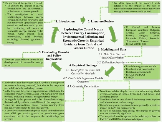
1. Introduction

Conventional energy sources based on oil, coal, and natural gas have demonstrated to be highly effective drivers of economic development [1]. Adams, et al. [2] showed that a 10% rise in non-renewable energy consumption will cause growth to increase by 2.11%, although a 10% surge in renewable energy consumption will determine an increase of growth by 0.27%. Therewith, Gozgor, et al. [3] noticed that both forms of energy sources are vital for the economic growth since renewable- and non-renewable energy consumption positively influence economic growth. Nevertheless, the concerns regarding instability of oil prices, the reliance on external energy sources, as well as the ecological consequences of pollutant emissions are substantial factors as regards the shift to renewable energy sources [4]. Hence, Al-Mulali, et al. [5] claimed that renewable electricity consumption is more substantial than non-renewable electricity consumption in promoting economic growth in Latin American states. Ito [6] emphasized that in the long run, renewable energy consumption positively influences economic growth, whereas a negative linkage was acknowledged between non-renewable energy consumption and growth. In the same vein, Bhattacharya, et al. [7] explored 38 top renewable energy consuming countries and confirmed the positive effect of renewable energy consumption on economic growth for 57% of the selected nations. Inglesi-Lotz [8] noticed for all the OECD nations that a 1% rise of renewable energy consumption will increase gross domestic product (hereinafter “GDP”) by 0.105% and GDP per capita by 0.100%. Rafindadi and Ozturk [9] reinforced that a 1% rise in renewable energy consumption surges German economic growth by 0.2194%. However, ecologically strategies to decrease the consumption of non-renewable energy may be unfavorable for growth in most of the emerging states since the share of renewable energy consumption in total energy consumption is fewer than in developed nations [10].

The amplified energy consumption is regularly viewed as the basis of ecological issues such as local air and water pollution, along with climate change, which harmfully affects human health and livelihoods [11]. Sustainable development, as one of the foremost aims of each economy, stimulates policymakers to use energy sources that release the fewest pollutants to the atmosphere [12]. Hence, succeeding the conversion from wood to coal, afterwards to oil & gas, the forthcoming will live the third foremost revolution from oil & gas to new energy [13]. Renewable energies may, in the long term, generate economic sustainability, seeing as energy from depleting resources is limited as more time passes. Likewise, renewable energy sources lessen carbon dioxide emanations, ensure the environment protection, diminish dependence on foreign sources and contribute to a rise in employment [14].

In the light of these facets, the purpose of this paper is twofold: to explore the impact of energy consumption and environmental pollution on economic growth, followed by the investigation of causal relationships between them, for a panel dataset of 11 Central and Eastern European countries (hereinafter “CEECs”), using data spanning the period 2000–2016. The reason for choosing CEECs as sample is that this region reveals a large unexploited renewable energy potential. As such, in 2017, Bulgaria, Czech Republic, Estonia, Croatia, Hungary, Lithuania and Romania have already reached the share corresponding to their compulsory target of 20% [15] final energy consumption from renewable sources by 2020 [16]. However, all selected CEECs are extremely reliant on Russian gas supplies, registering restricted internal production, except Romania. At the same time, the national markets vary in size and energy consumption. For instance, the energy consumed in Poland exceeds the total energy consumed in the Czech Republic, Hungary and Slovakia. A suitable energy combination is registered in Slovakia, but Poland and the Czech Republic depend to a great extent on coal, whereas Hungary hinge largely on nuclear power. Romania owns greater indigenous sources, primarily natural gas and coal, Estonia produces energy mostly from oil shale, whilst Latvia shows a high level of renewables (37%) [17].

The contribution of this paper to scientific knowledge is as follows. First, even if there prevails a wide empirical literature on energy consumption - economic growth nexus, there are a few papers investigating this relationship for CEECs. Merely Marinas, et al. [18] explored the causal relation between renewable energy and economic growth in CEECs. Hence, there seems to be a research gap in this field. Besides, previous papers employed either the percentage of renewable energy sources in gross inland energy consumption [19,20,21], biomass energy consumption [22,23,24,25,26] or hydroelectricity consumption [27] in order to catch the renewable energy consumption. Second, unlike earlier studies, present paper investigates the causal associations between energy consumption, both renewable and non-renewable, greenhouse gases emissions and economic growth by considering all forms of renewable energy, namely: hydro power, wind power, solar photovoltaic, solid biofuels, excluding charcoal, geothermal energy. As well, alternative & nuclear, along with the fossil fuel energy consumption are covered. Third, this study provides researchers with novel viewpoints for the energy-growth nexus since, to the best of our knowledge, there is not prior evidence on the relationship between renewable energy (both overall and by type), non-renewable energy, greenhouse gases emissions and economic growth in the CEECs. The CEECs passed through the transformation from the centrally planned economy, based on the state possession to the market economy based on the supremacy of private ownership. Hence, this paper has significant implications for the establishment of upcoming policies on promoting renewable energies in conjunction with macroeconomic policies. To account for the historic evolution of these states from communism to capitalism and democracy, two noteworthy control variables are included, namely economic freedom, as well as political stability and absence of violence/terrorism.

In this frame, the rest of the paper is arranged as follows. The second section discusses the literature on current topic. The third section presents sample, variables and quantitative methods. The estimation results are provided in the fourth section. The final section assesses the key findings and formulates policy recommendations.

2. Literature Review

Energy is vital for growth since production is a function of capital, labor, and energy [28]. The relation between energy and economic growth suggests four hypotheses: feedback, growth, conservation and neutral [25,29,30,31]. Feedback hypothesis [10,20,23,30,32,33,34,35,36,37] assumes that there occurs a causal relation between energy consumption and economic growth. Conservation hypothesis [10,23,36,37,38,39,40] shows movement in one direction initiated from growth to energy consumption. Growth hypothesis [10,23,25,34,36,37,39,41] supposes unidirectional causal relation moving from energy to economic growth. Neutrality hypotheses [10,19,32,34,37,38,41] reveal the lack of causal relation between energy consumption and economic growth.

Country-specific studies for nations such as Brazil [42], Canada [43], China [39,44,45,46], France [47], Germany [9], Greece [48], India [30], Iran [49], Malaysia [50], Pakistan [29] or Russia [51], have revealed that the outcomes concerning the causal relationship between energy consumption and economic growth is contradictory and mixed [52]. For instance, Payne [25] found for the US over the period 1949–2007 there was a unidirectional causality from biomass energy consumption to real GDP. Bildirici [26] found for transition countries a two-way causality among biomass energy consumption and economic growth both in the long-run and in the strong causality. Azlina and Mustapha [50] concluded for Malaysia during 1970–2010 unidirectional causal relations from economic growth to energy consumption, from pollutant emissions to energy consumption and from pollutant emissions to economic growth. Georgantopoulos [48] noticed a unidirectional causality from electricity consumption to real GDP in Greece, over 1980–2010. For the case of Brazil, Carpio [42] identified a long-term equilibrium association between GDP and electricity consumption. Hu, Guo, Wang, Zhang and Wang [39] documented for Chinese industrial sectors a short-run one-way causal link from economic growth to energy consumption, but a long-run unidirectional causal association from energy consumption to economic growth. Zaman, et al. [53] provided evidence that renewable energy consumption increases gross domestic product per capita in Brazil, India, China and South Africa. Cheratian and Goltabar [49] revealed a bidirectional causality between industrial energy consumption and Iranian regional growth. Taghizadeh-Hesary, et al. [54] pointed out that Japanese GDP growth rate have increased the consumption of crude oil, but economic declines have had the effect of falling oil consumption. Luqman, Ahmad and Bakhsh [29] found for Pakistan that renewable energy, as well as nuclear energy consumption shows a positive and asymmetric linkages with real GDP. On the contrary, Ocal and Aslan [40] documented that renewable energy consumption negatively influences economic growth in Turkey, providing evidence for a one-way causality running from economic growth to renewable energy consumption. Besides, Burakov and Freidin [51] noticed for Russia over 1990–2014 that renewable energy consumption does not Granger causes economic growth or financial development. Bulut and Muratoglu [31] confirmed the lack of causality between GDP and renewable energy consumption in Turkey.

Further, also multi-country studies employed for groups such as ASEAN-5 [38], Asia-Pacific Economic Cooperation (hereinafter “APEC”) [33], Black Sea and Balkan [34], BRICS [23], CEECs [18], emerging countries [41], EU member nations [14,20], G7 [37], MENA region [21,55], OECD [4,8,32,35,56], South America nations [57], Sub-Saharan African states [2] or West Africa [22], documented inconsistent results [52]. Hence, Tugcu, Ozturk and Aslan [37] explored G7 nations over 1980–2009 and found a short-run causal relationship from non-renewable energy consumption to economic growth in Japan, whilst the lack of causality for other states. Kahia, Ben Aissa and Charfeddine [55] emphasized for MENA Net Oil Exporting Countries a short-run unidirectional causality from economic growth to renewable energy consumption, but a long-run bidirectional causality. Rosado and Sánchez [57] noticed a long-run bidirectional causal link between CO2 emissions and GDP per capita, as well as a one-way causal relation from electric power consumption to CO2 emissions and GDP per capita in 10 South American countries, during 1980–2012. Narayan and Doytch [36] investigated 89 countries over 1971–2011 and found that economic growth positively influences the consumption of renewables only for the low and lower middle-income states. Obradovic and Lojanica [58] revealed no short-run causality between energy and economic growth in Greece and Bulgaria, but long-run causality from energy and CO2 emissions to economic growth in both states. Marinas, Dinu, Socol and Socol [18] validated in the long-run the bi-directional causality between renewable energy consumption and economic growth. For a panel data of 28 European Union nations, Akadiri, Alola, Akadiri and Alola [20] provided evidence for a long-run bidirectional causal association between renewable energy consumption and economic growth. In contrast, Menegaki [19] showed the lack of short- or long-run causality from renewable energy consumption to economic growth for 27 European countries.

The topic of energy consumption and economic growth was also explored for the case of South-Eastern European countries or European transition nations. Ozturk and Acaravci [59] proved a long-run relationship between energy use per capita and real GDP per capita, as well as two-way causal associations merely in Hungary, whereas for Albania, Bulgaria and Romania equilibrium connections not occurred. For nine Black Sea and Balkan countries, Kocak and Sarkgunesi [34] concluded that renewable energy consumption has a positive effect on economic growth. Bildirici and Ozaksoy [24] revealed short-run unidirectional causality from economic growth to biomass energy consumption for Albania, but one-way causality from biomass energy consumption to economic growth in Bulgaria and Romania. Besides, both in the short-run and long-run, unidirectional causal relations from economic growth to biomass energy consumption were established in Bosnia and Herzegovina, Czech Republic, Hungary, Macedonia and Slovak Republic.

Another branch of literature is oriented towards the environment quality or related pollutants, respectively the investigation of the environmental Kuznets curve (hereinafter “EKC”) which claims an inverted-U association among pollution and economic development. For instance, Lu [60] provided evidence for a quadratic relation among greenhouse gas emissions, energy consumption and economic growth, consistent with the EKC for 16 Asian countries, over 1990–2012. Hamit-Haggar [43] found a statistically significant non-linear association between greenhouse gas emissions and economic growth for Canadian industrial sectors over 1990–2007. Also Yao, et al. [61] confirmed the EKC for 17 major developing and developed nations during 1990–2014. As opposed, Adu and Denkyirah [62] did not confirm the EKC in West Africa.

Thus, no clear agreement has occurred with reference to the impact of the use of renewable energy sources or non-renewable energy sources on economic growth due to variances in methodological approaches, model description, number of selected variables, quantitative techniques, and the data [27,40,52].

Table 1. Summary of previous related studies.

Study	Period	Dataset	Quantitative Methods	Empirical Findings
Alam and WahidMurad [56]	1970–2012	25 OECD nations	Autoregressive distributed lag (ARDL), pooled mean group (PMG), mean group (MG) and dynamic fixed effect (DFE)	Economic growth drives renewable energy use in the long-term, but a contrary outcome ensues in the short-term
Aydin [23]	1992–2013	BRICS states	Bootstrap panel causality	Biomass energy positively influence economic growth in all countries, except Brazil
Aydin [32]	1980–2015	26 OECD states	Dumitrescu-Hurlin and Panel frequency causality tests	No causality among economic growth and renewable electricity consumption Bidirectional temporary, and permanent causality among renewable-nonrenewable electricity consumption and economic growth
Bao and Xu [44]	1997–2015	30 provinces in China	Bootstrap panel causality	No causality between renewable energy consumption and economic growth in 53% of provinces and 43% of geographical regions
Charfeddine and Kahia [21]	1980–2015	MENA region	Panel vector autoregressive	Weak positive impacts of renewable energy consumption on economic growth
Chen, Zhao, Lai, Wang and Xia [45]	1995–2012	30 provinces of China	Panel Granger causality	Bidirectional causalities among renewable energy, CO2 emissions and economic growth
Eren, Taspinar and Gokmenoglu [30]	1971–2015	India	Dynamic ordinary least squares, Granger causality test under VECM	Bidirectional causality amid renewable energy consumption and economic growth
Fan and Hao [46]	2000–2015	31 Chinese provinces	Vector error-correction model	Renewable energy consumption per capita growth rate is not a Granger cause of economic growth neither long-term nor short-term
Kahouli [35]	1990–2015	34 OECD nations	OLS pooled, within, GLS, 3SLS, GMM	A 1% increase in energy consumption rises the economic growth by 0.12% and 0.017% respectively
Maji and Sulaiman [22]	1995–2014	15 West African states	Panel dynamic ordinary least squares	Renewable energy use is negatively linked to the economic growth
Mohamed, Ben Jebli and Ben Youssef [47]	1980–2015	France	Autoregressive distributed lag (ARDL)	Short-run unidirectional causality running from renewable energy consumption to GDP, whereas bidirectional causality in the long-run
Ozcan and Ozturk [41]	1990–2016	17 emerging states	Bootstrap panel causality	No association between renewable energy consumption and economic growth in 16 states One-way causality running from renewable energy consumption to real GDP in Poland
Tuna and Tuna [38]	1980–2015	ASEAN-5 countries	Symmetric and asymmetric causality analysis	Economic growth and renewable energy consumption are not connected Significant connection between non-renewable energy consumption and economic growth
Zafar, Shahbaz, Hou and Sinha [33]	1990–2015	APEC states	Heterogenous causality analysis	Bidirectional causal relations between economic growth, renewable energy consumption, and non-renewable energy consumption

Source: Authors’ work based on the literature review.

provides a brief review of the most recent studies in the field.

3. Modeling and Data

3.1. Data Selection and Variable Description

The database covers 11 Central and Eastern European countries, namely: Bulgaria, Croatia, Czech Republic, Estonia, Hungary, Latvia, Lithuania, Poland, Romania, Slovakia and Slovenia. The timeframe was constrained by the availability of data. Hence, the data set covers the period 2000–2016 common for all the variables. Following previous studies in this area [3,6,8,9,10,11,19,24,26,27,30,34,36,45,46,47,49,53,55,56,58,59,60,61,62], gross domestic per capita growth was selected as measure for economic growth. As well, the multivariate framework encompasses variables towards renewable energy, both overall [2,3,4,6,7,8,9,10,14,18,19,20,29,30,31,32,33,34,36,37,38,40,41,44,45,46,47,51,55,56,61] and by type [22,23,24,25,26,27], alternative & nuclear energy [29,53], non-renewable energy [2,3,7,10,27,32,33,36,37,38,45,55], fossil fuel energy [6,31,47], environmental pollution [6,19,20,27,29,35,42,43,45,50,55,58,60,61,62]. Besides, country-level controls are covered concerning energy intensity [11], energy dependence, trade [5,11,33,35,47,56,62], domestic credit to private sector [11,55], urban population [35,44], economic freedom, political stability and absence of violence/terrorism [11,22]. The selected variables used for estimation purpose, along with their definition, measurement, source and period availability are presented in

Table 2. Variables’ presentation.

Variables	Definitions	Unit of Measurement	Source	Data Availability
Variables regarding economic growth
GROWTH	Annual percentage growth rate of GDP per capita based on constant local currency. Aggregates are based on constant 2010 U.S. dollars	%	World Bank (NY.GDP.PCAP.KD.ZG)	1961–2018
Variables regarding renewable energy
Overall
REC	Renewable energy consumption (% of total final energy consumption). Renewable energy consumption is the share of renewable energy in total final energy consumption	%	World Bank (EG.FEC.RNEW.ZS)	1990–2015
			Eurostat (nrg_ind_335a)	2004–2016
By type of renewable energy
GIC_RE	Gross inland consumption of renewable energies (logarithmic values)	Thousand tonnes of oil equivalent (TOE)	Eurostat (nrg_107a)	1990–2016
GIC_HP	Gross inland energy consumption - Hydro power (logarithmic values)	Thousand tonnes of oil equivalent (TOE)	Eurostat (nrg_107a)	1990–2016
GIC_WP	Gross inland energy consumption - Wind power (logarithmic values)	Thousand tonnes of oil equivalent (TOE)	Eurostat (nrg_107a)	1990–2016
GIC_SP	Gross inland energy consumption - Solar photovoltaic (logarithmic values)	Thousand tonnes of oil equivalent (TOE)	Eurostat (nrg_107a)	1990–2016
GIC_SB	Gross inland energy consumption - Solid biofuels, excluding charcoal (logarithmic values)	Thousand tonnes of oil equivalent (TOE)	Eurostat (nrg_107a)	1990–2016
GIC_GE	Gross inland energy consumption - Geothermal energy (logarithmic values)	Thousand tonnes of oil equivalent (TOE)	Eurostat (nrg_107a)	1990–2016
Variables regarding alternative & nuclear energy
ANE	Alternative & nuclear energy (% of total energy use). Clean energy is noncarbohydrate energy that does not produce carbon dioxide when generated. It includes hydropower and nuclear, geothermal, and solar power, among others	%	World Bank (EG.USE.COMM.CL.ZS)	1990–2015
Variables regarding non-renewable energy
GIC_NRE	Gross inland consumption - Waste, non-renewable (logarithmic values)	Thousand tonnes of oil equivalent (TOE)	Eurostat (nrg_108a)	1990–2016
Variables regarding fossil fuel energy
FFEC	Fossil fuel energy consumption (% of total). Fossil fuel comprises coal, oil, petroleum, and natural gas products.	%	World Bank (EG.USE.COMM.FO.ZS)	1960–2015
FCSFF	Final consumption of solid fossil fuels (logarithmic values)	Thousand tonnes	Eurostat (nrg_cb_sff)	1990–2017
Variables regarding environmental pollution
GHG	Greenhouse gases emissions (CO2, N2O in CO2 equivalent, CH4 in CO2 equivalent, HFC in CO2 equivalent, PFC in CO2 equivalent, SF6 in CO2 equivalent, NF3 in CO2 equivalent). All sectors and indirect CO2 (excluding LULUCF and memo items, including international aviation) (logarithmic values)	Million tonnes	Eurostat (env_air_gge)	1985–2017
Country-level control variables
EI	Energy intensity which measures the energy consumption of an economy and its energy efficiency. It is the ratio between gross inland consumption of energy and GDP (logarithmic values)	Kilograms of oil equivalent (KGOE) per thousand euro	Eurostat (nrg_ind_ei)	1990–2017
ED	Energy dependence which shows the extent to which an economy relies upon imports in order to meet its energy needs. It is calculated as net imports divided by the sum of gross inland energy consumption plus maritime bunkers.	%	Eurostat (t2020_rd320)	1990–2016
TRADE	Trade (% of GDP). Trade is the sum of exports and imports of goods and services measured as a share of gross domestic product.	%	World Bank (NE.TRD.GNFS.ZS)	1960–2018
DCPS	Domestic credit to private sector (% of GDP). IT refers to financial resources provided to the private sector by financial corporations, such as through loans, purchases of nonequity securities, and trade credits and other accounts receivable, that establish a claim for repayment.	%	World Bank (FS.AST.PRVT.GD.ZS)	1960–2018
UP	Urban population (% of total population)	%	World Bank (SP.URB.TOTL.IN.ZS)	1960–2018
EF	Economic freedom	Score	The Heritage Foundation	1995–2019
PS	Political Stability and Absence of Violence/Terrorism which measures perceptions of the likelihood of political instability and/or politically-motivated violence, including terrorism	Ranges from −2.5 (weak) to 2.5 (strong) governance	World Bank (Worldwide Governance Indicators)	1996–2017

Source: Authors’ work based on Eurostat and World Bank descriptions.

.

3.2. Estimation Procedure

With the purpose of exploring the impact of energy consumption and environmental pollution on economic growth, the empirical analysis will proceed with the estimation of panel data regression models as in prior studies [6,8,22,35,36], with fixed and random effects, having the following general specification:

$$GROWT{H}_{it}={\alpha }_0+{\gamma }_1\times ENERG{Y}_{it}+{\gamma }_2\times GH{G}_{it}+{\gamma }_3\times CONTROL{S}_{it}+{\epsilon }_{it}$$

(1)

i = 1, 2, …, 11; t = 2000, …, 2016

where the dependent variable is GDP per capita growth rate. ENERGY means a vector of explanatory variables concerning each type of energy, namely renewable energy, alternative & nuclear energy, non-renewable energy, fossil fuel energy. GHG reveals the pollutant emissions. CONTROLS describe the country-level control measures. ${\alpha }_0$ means the country-specific intercept, ${\gamma }_1$–${\gamma }_3$ are the coefficients to be estimated, ε is the disturbance term, i is the subscript of CEECs, and t is the subscript of time and consider the unobservable time-invariant individual specific effect, not covered in the regression.

Therewith, aiming to investigate potential non-linear associations between energy consumption, environmental pollution and economic growth, the squared term of ENERGY (hereinafter “ENERGY_SQ”) will be included in Equation (1):

$$\begin{array}{c}GROWT{H}_{it}={\alpha }_0+{\gamma }_1\times ENERG{Y}_{it}+{\gamma }_2\times ENERGY\_S{Q}_{it}+{\gamma }_3\times GH{G}_{it}+\\ {\gamma }_4\times CONTROL{S}_{it}+{\epsilon }_{it}\end{array}$$

(2)

i = 1, 2, …, 11; t = 2000, …, 2016

Next, the unit root examination will be carried out to determine the stationarity of the variables. Alike previous studies [2,3,4,6,8,12,19,25,27,29,34,43,45,53,55,61], to ensure the robustness of the outcomes, several tests are employed, respectively: Levin, Lin and Chu (hereinafter “LLC”), Im, Pesaran and Shin (hereinafter “IPS”), Augmented Dickey-Fuller (hereinafter “ADF”), Phillips–Perron (hereinafter “PP”) and Breitung. The ADF and PP supposes the following regression [62]:

$$\Delta X_t=\alpha +\alpha X_{t-1}+{{\displaystyle \sum }}_{i=1}^m{\gamma }_i\Delta X_{t-1}+{\epsilon }_t$$

(3)

where ∆ reveals the first-difference operator, m is the optimal lagged length, ${\gamma }_i$ is the time trend, β is parameter estimate, α is the constant parameter and ${\epsilon }_t$ is the stationary random error. The null hypothesis supposes that β = 0, whilst the alternative hypothesis claims that β ≠ 0. The hypothesis of unit root is rejected if the parameter is not statistically significant.

Like in Yao, Zhang and Zhang [61], the LLC is presented as follows:

$$\Delta y_{it}=\rho y_{it-1}={{\displaystyle \sum }}_{L=1}^{p_i}{\theta }_{iL}\Delta y_{it-L}={\alpha }_{mi}{d}_{mt}={\epsilon }_{it}$$

(4)

where ∆ denotes the first differential operator, $d_m$ a vector of deterministic variables and ${\alpha }_m$ a vector of coefficients, for the model m = $\left\{1, 2, 3\right\}$. The null hypothesis is ρ = 0 and the alternative hypothesis is ρ < 0, the rejection of the null implying that the panel is stationary.

In case of IPS test, ρ may vary across panels, whilst the null hypothesis is similar to LLC, but the alternative hypothesis is ρ < 0 for at least one. The panel data is stationary if the regression results reject the null hypothesis. Equation (4) is transformed as shown below:

$$\Delta y_{it}={\rho }_i{y}_{it-1}={{\displaystyle \sum }}_{L=1}^{p_i}{\theta }_{iL}\Delta y_{it-L}={\alpha }_{mi}{d}_{mt}={\epsilon }_{it}$$

(5)

After panel unit root tests provide evidence that the variables are stationary, several panel cointegration tests are employed to establish the long-run connection among the variables, namely Pedroni [2,4,7,8,20,22,34,43,45,55,61], Kao [2,22,53,55] and Fisher (combined with Johansen) [20,46,53]. The Pedroni test permits for heterogeneous intercepts and trend coefficients across nations, as follows [5]:

$$y_{it}={\alpha }_i+{\delta }_{i}t+{\beta }_{1i}{x}_{1i,t}+{\beta }_{2i}{x}_{2i,t}+\dots +{\beta }_{Mi}{x}_{Mi,t}+{\epsilon }_{i,t}$$

(6)

where y and x are expected to be integrated in order one. The parameters ${\alpha }_i$ and ${\delta }_i$ are individual and trend effects. The residual ${\epsilon }_{i,t}$ is integrated in order one under the null hypothesis of no cointegration. The null hypothesis of the Pedroni cointegration is that there is no cointegration. Besides, the Kao residual cointegration test is based on a Monte Carlo procedure, which outclasses the test of Pedroni when there is a small timeseries length in panel data [63].

Beyond settling the cointegration associations, the cointegration coefficients of the explanatory variables can be estimated through the fully modified ordinary least squares (hereinafter “FMOLS”) [2,4,7,20,22,26,33,34,43,45,53,55,61] and dynamic ordinary least squares (hereinafter “DOLS”) regressions [2,7,22,30,31,34,45,53,61]. The FMOLS corrects for both the endogeneity bias and serial correlation, and allow for consistent and efficient estimators of the long-run association [43], whereas DOLS corrects for endogeneity in regressors and serial correlation in errors using leads and lags of first differences and generalized least squares procedures [2]. In line with Bildirici [26], Chen, Zhao, Lai, Wang and Xia [45], the panel FMOLS estimation appears as follows:

$${\widehat{\beta }}_{GFM}={\left[{{\displaystyle \sum }}_{i=1}^N{{\displaystyle \sum }}_{t=1}^T\left(x_{it}-{\overline{x}}_i\right){(x_{it}-{\overline{x}}_i)}^{\prime }\right]}^{-1}\left[{{\displaystyle \sum }}_{i=1}^N({{\displaystyle \sum }}_{t=1}^T\left(x_{it}-{\overline{x}}_i\right){\widehat{y}}_{it}^{+}-T{\widehat{\Delta }}_{\epsilon u}^{+}\right]$$

(7)

where ${\overline{x}}_i$ denotes the individual specific means, N reveals the cross-sectional dimension, T describes the time series, ${\widehat{y}}_{it}^{+}$ is the corresponding series corrected for endogeneity, ${\widehat{\Delta }}_{\epsilon u}^{+}$ specifies the correction term. The between-dimension estimator and the related t-statistic are showed below [24,45,57,61], where ${\beta }_{FM,i}$ is the conventional FMOLS estimator of the i-th panel member:

$${\widehat{\beta }}_{GFM}=N^{-1}{{\displaystyle \sum }}_{i=1}^N{\beta }_{FM,i}$$

(8)

$$t_{{\beta }_{GFM}}=N^{-1/2}{{\displaystyle \sum }}_{i=1}^N{t}_{{\beta }_{FM,i}}$$

(9)

As well, the DOLS estimator, along with the associated t-statistic are described below [57], where ${\beta }_{D,i}$ is the conventional DOLS estimator corresponding to i-th panel member:

$${\widehat{\beta }}_{GD}=N^{-1}{{\displaystyle \sum }}_{i=1}^N{\beta }_{D,i}$$

(10)

$$t_{{\beta }_{GD}}=N^{-1/2}{{\displaystyle \sum }}_{i=1}^N{t}_{{\beta }_{D,i}}$$

(11)

Further, the panel vector error correction model (hereinafter “PVECM”) is employed as in earlier papers [30,46,47] to inspect the association amongst renewable energy, non-renewable energy, greenhouse gases emissions and economic growth from the standpoint of long-term equilibrium link and short-term dynamic connection. The panel Granger causality [4,19,30,43,47,55] is inspected for six different models, where RE changes depending on the form of renewable energy (GIC_RE, GIC_HP, GIC_WP, GIC_SP, GIC_SB, GIC_GE) and is written in line with [43]:

$$\begin{array}{l}(1-L)\left[\begin{array}{c}GROWT{H}_{it}\\ R{E}_{it}\\ GIC\_NR{E}_{it}\\ GH{G}_{it}\end{array}\right]=\left[\begin{array}{c}{\alpha }_{1j}\\ {\alpha }_{2j}\\ {\alpha }_{3j}\\ {\alpha }_{4j}\end{array}\right]+{{\displaystyle \sum }}_{q=1}^p\left(1-L\right)\left[\begin{array}{cccc}{\psi }_{{11}_{iq}},& {\psi }_{{12}_{iq}},& {\psi }_{{13}_{iq}},& {\psi }_{{14}_{iq}}\\ {\psi }_{{21}_{iq}},& {\psi }_{{22}_{iq}},& {\psi }_{{23}_{iq}},& {\psi }_{{24}_{iq}}\\ {\psi }_{{31}_{iq}},& {\psi }_{{32}_{iq}},& {\psi }_{{33}_{iq}},& {\psi }_{{34}_{iq}}\\ {\psi }_{{41}_{iq}},& {\psi }_{{42}_{iq}},& {\psi }_{{43}_{iq}},& {\psi }_{{44}_{iq}}\end{array}\right]\\ \left[\begin{array}{c}GROWT{H}_{it-q}\\ R{E}_{it-q}\\ GIC\_NR{E}_{it-q}\\ GH{G}_{it-q}\end{array}\right]+\left[\begin{array}{c}{\xi }_{1i}\\ {\xi }_{2i}\\ {\xi }_{3i}\\ {\xi }_{4i}\end{array}\right]EC{T}_{t-1}+\left[\begin{array}{c}{\omega }_{1it}\\ {\omega }_{2it}\\ {\omega }_{3it}\\ {\omega }_{4it}\end{array}\right]\end{array}$$

(12)

where L is a lag operator, q is the lag length set according to Schwarz information criterion, ${\omega }_{it}$ are the serially uncorrelated error term and ξ is the speed of adjustment. If the null hypothesis, ${\psi }_{{12}_{iq}}$= 0 ∀ _iq is rejected, short-run causality runs from ΔRE to ΔGROWTH. Analogous, if ${\psi }_{{21}_{iq}}$ = 0 ∀ _iq is rejected, short-run causality runs from ΔGROWTH to ΔRE. Besides, if the joint null hypothesis ${\psi }_{{13}_{iq}}$ = ${\psi }_{{14}_{iq}}$ = 0 ∀ _iq is rejected, short-run causality runs from ∆GIC_NRE and ∆GHG to ΔGROWTH. As regards the long-run causality, we the coefficient of the error correction term (hereinafter “ECT”) is checked.

4. Empirical Findings

4.1. Descriptive Statistics and Correlation Analysis

The descriptive statistics for the selected variables are presented in

Table 3. Descriptive statistics (raw data).

Variables	Obs.	Mean	Std. Dev.	Min	Max
GROWTH	187	3.74	4.29	−14.56	12.92
REC	187	17.13	8.47	3.73	38.70
GIC_RE	187	2207.11	1882.50	488.10	8970.40
GIC_HP	187	334.67	385.26	0.40	1737.50
GIC_WP	187	50.94	144.92	0.00	1082.40
GIC_SP	187	14.31	41.26	0.00	194.70
GIC_SB	187	1646.64	1462.48	91.30	6987.70
GIC_GE	187	16.44	27.54	0.00	119.90
ANE	171	14.16	10.79	0.02	44.32
GIC_NRE	187	76.12	112.93	0.00	741.50
FFEC	171	69.88	17.60	13.06	96.25
FCSFF	187	2951.13	5860.30	26.00	22,050.00
GHG	187	87.37	109.34	10.59	419.89
EI	187	308.93	109.98	175.98	778.63
ED	187	43.52	17.51	6.80	81.80
TRADE	187	115.85	32.33	58.08	184.55
DCPS	185	47.38	19.25	0.19	101.29
UP	187	62.99	7.58	50.75	74.33
EF	187	64.93	6.49	47.30	78.00
PS	165	0.69	0.31	0.00	1.30

Source: Authors’ computations. Notes: For the definition of variables, please see Table 2.

. The mean share of renewable energy in total final energy consumption over the period 2000–2016 is 17.13%, which is below the targeted threshold of minimum 27% that should be reachable before 2030 [64].

As regards the types of renewable energy, the figures reveal that the gross inland consumption of solid biofuels and hydro power show the highest mean values, while the gross inland consumption of wind, geothermal and solar photovoltaic power register the lowest average levels out of all renewable energies. As a consequence of these findings, CEECs should consider investing even further in hydro electricity production, as it is non-polluting, durable, although expensive when seeing the structures and equipment that need to be purchased in order to be obtained. Biogasoline is also a non-polluting option for energy resources, with a more cost-efficient approach.

Further, Figure 1 provides evidence that the mean values concerning the share of renewable energy consumption tend to be higher than 20 % in three member states, namely Estonia, Croatia and Latvia.

By form of renewable energies, Figure 2 reveals that the gross inland energy consumption of solid biofuels is at outstanding levels in Poland and Romania. Romania also has the highest consumption of hydro power, but uses moderate levels of geothermal and photovoltaic power. The leader in geothermal energy consumption is Hungary, and top consumer for photovoltaic energy is the Czech Republic.

When comparing renewable energies and wasted, non -renewable energies, Figure 3 points out that the renewable energy levels are higher in every analyzed country, outmatching waste energy. The top leaders in renewable energy vs. waste energy are yet again Poland and Romania. In addition, Poland seems to have most non-renewable energy consumption among the entire CEECs. Besides, the Czech Republic is the second largest consumer of waste, non-renewable energy resources.

Table 4. Correlation matrix.

Variables	GROWTH	REC	GIC_RE	GIC_HP	GIC_WP	GIC_SP	GIC_SB	GIC_GE	ANE	GIC_NRE
GROWTH	1
REC	−0.1	1
GIC_RE	−0.07	−0.16 *	1
GIC_HP	−0.04	0.13 †	0.41 ***	1
GIC_WP	−0.04	−0.00	0.69 ***	0.17 *	1
GIC_SP	−0.11	−0.01	0.25 ***	0.15 *	0.25 ***	1
GIC_SB	−0.05	−0.20 **	0.98 ***	0.26 ***	0.65 ***	0.14 †	1
GIC_GE	0.06	−0.03	0.12 †	−0.07	0.1	0	0.13 †	1
ANE	−0.01	−0.22 **	−0.38 ***	−0.06	−0.21 **	0.19 *	−0.44 ***	0.13 †	1
GIC_NRE	−0.04	−0.33 ***	0.76 ***	−0.04	0.62 ***	0.22 **	0.78 ***	0.05	−0.22 **	1
FFEC	0.03	−0.37 ***	0.55 ***	0.31 ***	0.18 *	0.07	0.53 ***	0.20 **	0.03	0.45 ***
FCSFF	−0.01	−0.43 ***	0.68 ***	−0.11	0.39 ***	−0.02	0.78 ***	−0.08	−0.37 ***	0.73 ***
GHG	0.02	−0.42 ***	0.81 ***	0.08	0.45 ***	0.04	0.88 ***	0.02	−0.38 ***	0.76 ***
EI	0.22 **	−0.31 ***	−0.19 **	−0.08	−0.16 *	−0.08	−0.17 *	−0.09	0.17 *	−0.12 †
ED	0.03	0.09	−0.48 ***	−0.24 **	−0.26 ***	−0.20 **	−0.49 ***	0.15 *	0.40 ***	−0.33 ***
TRADE	−0.03	0.01	−0.38 ***	−0.47 ***	−0.14 †	0.21 **	−0.38 ***	0.29 ***	0.28 ***	−0.04
DCPS	−0.34 ***	0.40 ***	−0.20 **	−0.26 ***	0.02	0.02	−0.20 **	−0.01	−0.13 †	−0.1
UP	0.03	−0.06	−0.16 *	−0.59 ***	−0.08	0.18 *	−0.07	0.11	−0.06	0.04
EF	−0.11	0.12	−0.15 *	−0.50 ***	0.11	0.18 *	−0.1	−0.04	−0.06	0.03
PS	0.04	−0.27 ***	−0.18 *	−0.50 ***	−0.13 †	−0.04	−0.13 †	−0.05	0.22 **	0.19 *
Variables	FFEC	FCSFF	GHG	EI	ED	TRADE	DCPS	UP	EF	PS
FFEC	1
FCSFF	0.54 ***	1
GHG	0.61 ***	0.96 ***	1
EI	−0.1	0	0.03	1
ED	0.04	−0.46 ***	−0.52 ***	−0.22 **	1
TRADE	−0.43 ***	−0.35 ***	−0.40 ***	−0.21 **	0.33 ***	1
DCPS	−0.43 ***	−0.23 **	−0.31 ***	−0.32 ***	0.08	0.35 ***	1
UP	−0.21 **	0.04	−0.03	0.41 ***	−0.11	0.24 ***	0.11	1
EF	−0.60 ***	−0.08	−0.17 *	−0.12	−0.06	0.58 ***	0.38 ***	0.54 ***	1
PS	−0.04	0.1	−0.03	−0.39 ***	0.27 ***	0.42 ***	0.02	−0.05	0.22 **	1

Source: Authors’ computations. Notes: Superscripts ***, **, *, and † indicate statistical significance at 0.1%, 1%, 5%, and 10% respectively. For the definition of variables, please see Table 2.

reveals the correlations between the variables.

This table suggest high correlations between GIC_SB and GIC_RE (0.98), GIC_RE and GIC_NRE (0.76), GIC_RE and GHG (0.81), GIC_SB and GIC_NRE (0.78), GIC_SB and FCSFF (0.78), GIC_SB and GHG (0.88), GIC_NRE and FCSFF (0.73), GIC_NRE and GHG (0.76), FCSFF and GHG (0.96). In order to overcome the multicollinearity issue, the aforementioned variables will be included in distinct regression models.

4.2. Panel Data Regression Models Outcomes

At first glance, the outcomes of the Hausman test were examined in order to identify if either fixed or random effects are selected. Alike Inglesi-Lotz [8], the Hausman test supports that in almost all models, the fixed effects estimation is preferred. The results of the panel data regression models with reference to the influence of renewable and non-renewable energy on economic growth are presented in

Table 5. Panel data regression models towards the influence of renewable and non-renewable energy consumption on economic growth.

Variables	(1)		(2)		(3)		(4)		(5)		(6)
	FE	RE	FE	RE	FE	RE	FE	RE	FE	RE	FE	RE
REC	−0.02	0.02	0.05	0.16
	(−0.37)	(0.32)	(0.18)	(0.84)
REC_SQ			−0.00	−0.00
			(−0.27)	(−0.56)
GIC_RE					−8.79 ***	−2.17 *	−51.83 ***	−57.07 ***
					(−4.56)	(−1.98)	(−3.58)	(−4.60)
GIC_RE_SQ							2.80 **	3.58 ***
							(3.00)	(4.48)
GIC_NRE									−0.40	−0.33	−0.39	−0.68
									(−1.23)	(−1.18)	(−0.67)	(−1.19)
GIC_NRE_SQ											−0.00	0.08
											(−0.01)	(0.76)
GHG	21.69 ***	0.96	22.03 ***	−0.51
	(4.37)	(0.84)	(4.30)	(−0.97)
EI	1.91	7.25 **	1.76	3.75 *	6.37 †	3.28	4.92	−3.45 †	9.77 **	4.76 *	9.77 **	5.66 *
	(0.49)	(2.59)	(0.44)	(2.23)	(1.83)	(1.16)	(1.43)	(−1.82)	(2.70)	(2.04)	(2.69)	(2.25)
ED	0.02	0.06	0.01	0.01	0.02	0.01	−0.02	0.01	0.06	0.03	0.06	0.04
	(0.35)	(1.49)	(0.30)	(0.46)	(0.53)	(0.35)	(−0.37)	(0.27)	(1.23)	(0.76)	(1.23)	(1.03)
TRADE	0.07 **	0.05 **	0.07 **	0.01	0.15 ***	0.05 *	0.16 ***	0.02	0.10 ***	0.04 *	0.10 ***	0.05 *
	(3.01)	(2.62)	(2.93)	(0.38)	(5.43)	(2.39)	(6.03)	(1.42)	(3.57)	(2.29)	(3.39)	(2.35)
DCPS	−0.13 ***	−0.09 ***	−0.14 ***	−0.09 ***	−0.08 **	−0.09 ***	−0.07 **	−0.10 ***	−0.10 ***	−0.09 ***	−0.10 ***	−0.09 ***
	(−5.41)	(−3.72)	(−4.98)	(−4.12)	(−3.26)	(−3.82)	(−3.29)	(−5.10)	(−4.01)	(−3.84)	(−3.99)	(−3.81)
UP	−0.24	−0.18	−0.27	0.02	−0.40	−0.07	−0.25	0.25 ***	−0.86 *	−0.07	−0.86 *	−0.12
	(−0.63)	(−1.11)	(−0.68)	(0.36)	(−1.10)	(−0.52)	(−0.70)	(3.47)	(−2.27)	(−0.56)	(−2.23)	(−0.84)
EF	0.10	−0.05	0.10	−0.07	0.10	−0.12	−0.02	−0.29 ***	0.04	−0.12	0.04	−0.10
	(0.75)	(−0.46)	(0.78)	(−0.95)	(0.76)	(−1.10)	(−0.18)	(−3.32)	(0.28)	(−1.12)	(0.27)	(−0.89)
PS	2.48	2.01	2.44	1.95	2.61	1.48	1.43	−2.13 †	1.25	1.61	1.25	1.45
	(1.34)	(1.16)	(1.31)	(1.42)	(1.42)	(0.90)	(0.78)	(−1.67)	(0.64)	(1.01)	(0.64)	(0.86)
_cons	−87.28 *	−32.41	−86.04 *	−11.87	35.41	11.13	206.47 **	254.84 ***	−8.57	−13.22	−8.52	−17.48
	(−2.28)	(−1.58)	(−2.22)	(−1.01)	(1.02)	(0.48)	(3.12)	(4.68)	(−0.24)	(−0.87)	(−0.24)	(−1.04)
F statistic	9.30 ***		8.32 ***		10.76 ***		11.10 ***		7.40 ***		6.53 ***
R-sq. within	0.37		0.37		0.37		0.41		0.29		0.29
Hausman test Prob > chi2	0.0017		0.0000		0.0014		0.0000		0.1082		0.2668
Turning Point							9.25	7.96
Obs.	163.00	163.00	163.00	163.00	163.00	163.00	163.00	163.00	163.00	163.00	163.00	163.00
N Countries	11.00	11.00	11.00	11.00	11.00	11.00	11.00	11.00	11.00	11.00	11.00	11.00

Source: Authors’ computations. Notes: Superscripts ***, **, *, and † indicate statistical significance at 0.1%, 1%, 5%, and 10% respectively. Figures in brackets show t-statistic. FE denotes Fixed-effects (within) regression. RE denotes Random-effects GLS regression. For the definition of variables, please see Table 2.

.

The outcomes exhibit that there occurs a non-linear association between the gross inland energy consumption of renewable energies and economic growth. Accordingly, if the renewable energy consumption exceeds the threshold of 9.25% of total final energy consumption, its impact on GDP per capita growth rate turn out to be positive. Besides, the non-renewable energy consumption shows a negative influence on economic growth, but statistically insignificant. Therefore, this finding reinforces the positive influence of renewable energy on economic growth, even if after a certain threshold.

Table 6. Panel data regression models towards the influence of hydro power, wind power and solar photovoltaic on economic growth.

Variables	(1)		(2)		(3)		(4)		(5)		(6)
	FE	RE	FE	RE	FE	RE	FE	RE	FE	RE	FE	RE
GIC_HP	−3.43 **	−1.02 *	−6.67 **	−1.03
	(−2.61)	(−2.22)	(−3.26)	(−0.98)
GIC_HP_SQ			0.48 *	0.02
			(2.05)	(0.14)
GIC_WP					−0.36	−0.24	−0.74 *	−0.38
					(−1.59)	(−1.17)	(−2.32)	(−1.08)
GIC_WP_SQ							0.11 †	0.08
							(1.67)	(1.22)
GIC_SP									0.45 *	−0.19	0.53 †	0.26
									(2.12)	(−1.00)	(1.78)	(0.77)
GIC_SP_SQ											−0.03	−0.14
											(−0.40)	(−1.63)
GHG	22.01 ***	0.27	23.20 ***	−0.41	21.21 ***	−0.03	22.16 ***	−0.93 †	24.34 ***	−0.79 †	24.01 ***	−0.62
	(4.54)	(0.38)	(4.80)	(−0.91)	(4.30)	(−0.05)	(4.49)	(−1.89)	(4.83)	(−1.90)	(4.69)	(−1.45)
EI	1.70	3.49	1.55	1.91	0.67	3.35	1.16	2.71	4.01	2.58 †	4.02	2.24
	(0.45)	(1.61)	(0.42)	(1.32)	(0.17)	(1.48)	(0.29)	(1.62)	(1.03)	(1.75)	(1.03)	(1.51)
ED	0.00	0.04	−0.01	0.03	0.01	0.02	0.02	0.00	0.04	−0.00	0.04	−0.00
	(0.10)	(1.22)	(−0.32)	(0.89)	(0.31)	(0.64)	(0.36)	(0.02)	(0.88)	(−0.03)	(0.83)	(−0.20)
TRADE	0.08 **	0.02	0.08 ***	−0.00	0.08 **	0.03	0.08 ***	0.01	0.06 *	0.01	0.06 *	0.01
	(3.30)	(1.35)	(3.59)	(−0.23)	(3.28)	(1.63)	(3.37)	(0.37)	(2.57)	(0.63)	(2.60)	(0.85)
DCPS	−0.12 ***	−0.08 ***	−0.12 ***	−0.09 ***	−0.13 ***	−0.08 ***	−0.12 ***	−0.08 ***	−0.13 ***	−0.09 ***	−0.13 ***	−0.09 ***
	(−4.80)	(−3.61)	(−4.83)	(−4.32)	(−5.06)	(−3.33)	(−4.75)	(−3.64)	(−5.18)	(−4.17)	(−5.05)	(−4.05)
UP	−0.14	−0.10	−0.32	−0.01	−0.07	0.00	0.03	0.05	−0.20	0.03	−0.21	0.04
	(−0.37)	(−0.96)	(−0.83)	(−0.14)	(−0.17)	(0.00)	(0.07)	(0.81)	(−0.53)	(0.48)	(−0.55)	(0.71)
EF	0.05	−0.17	0.03	−0.16 †	0.12	−0.09	0.05	−0.09	0.11	−0.07	0.11	−0.08
	(0.36)	(−1.60)	(0.27)	(−1.95)	(0.89)	(−0.86)	(0.39)	(−1.13)	(0.86)	(−0.90)	(0.89)	(−0.97)
PS	2.13	0.69	1.80	0.14	2.87	1.21	2.53	1.19	2.49	0.94	2.54	0.85
	(1.18)	(0.44)	(1.00)	(0.10)	(1.56)	(0.79)	(1.37)	(0.89)	(1.37)	(0.76)	(1.39)	(0.69)
_cons	−74.34 *	4.54	−63.20 †	13.63	−91.40 *	−10.20	−100.46 **	−2.55	−113.63 **	−2.09	−112.21 **	−1.41
	(−2.00)	(0.27)	(−1.70)	(1.33)	(−2.45)	(−0.75)	(−2.68)	(−0.27)	(−2.94)	(−0.22)	(−2.88)	(−0.15)
F statistic	10.48 ***		10.06 ***		9.73 ***		9.14 ***		10.07 ***		9.03 ***
R-sq. within	0.40		0.41		0.38		0.39		0.39		0.39
Hausman test Prob > chi2	0.0001		0.0000		0.0001		0.0000		0.0000		0.0000
Turning Point			6.93				3.41
Obs.	163.00	163.00	163.00	163.00	163.00	163.00	163.00	163.00	163.00	163.00	163.00	163.00
N Countries	11.00	11.00	11.00	11.00	11.00	11.00	11.00	11.00	11.00	11.00	11.00	11.00

Source: Authors’ computations. Notes: Superscripts ***, **, *, and † indicate statistical significance at 0.1%, 1%, 5%, and 10% respectively. Figures in brackets show t-statistic. FE denotes Fixed-effects (within) regression. RE denotes Random-effects GLS regression. For the definition of variables, please see Table 2.

provides the empirical outcomes regarding the influence of hydro power, wind power and solar photovoltaic power on economic growth. Again, non-linear relationships are found. The required thresholds for a positive influence on GDP per capita growth rate are 6.93 thousand tonnes of oil equivalent for hydro power and 3.41 thousand tonnes of oil equivalent for wind power.

In the case of solar photovoltaic power, the influence on growth is positive. Hence, out of the three selected renewable energies, the solar power is the most profitable for the economy. Although photovoltaic systems are currently expensive, manufacturers often offer reasonable payment plans for the purchase of such systems. In the long run, this type of equipment, that converts solar power into energy, by using photovoltaic cells, may turn out to be least expensive one in the EU.

The estimation results concerning the influence of solid biofuels and geothermal energy on economic growth are reported in

Table 7. Panel data regression models towards the influence of solid biofuels, excluding charcoal and geothermal energy on economic growth.

Variables	(1)		(2)		(3)		(4)
	FE	RE	FE	RE	FE	RE	FE	RE
GIC_SB	−8.16 ***	−1.66	−20.42	−19.13
	(−4.31)	(−1.46)	(−1.60)	(−1.57)
GIC_SB_SQ			0.87	1.14
			(0.97)	(1.38)
GIC_GE					0.39	0.08	−0.26	−1.45
					(0.88)	(0.31)	(−0.19)	(−1.56)
GIC_GE_SQ							0.20	0.37 †
							(0.50)	(1.74)
GHG					22.07 ***	−0.87 †	21.86 ***	−0.58
					(4.45)	(−1.74)	(4.38)	(−1.09)
EI	6.36 †	4.23	5.61	3.87	1.80	3.07 *	2.08	3.82 *
	(1.81)	(1.47)	(1.56)	(1.23)	(0.46)	(2.10)	(0.53)	(2.55)
ED	0.02	0.02	0.01	0.01	0.02	0.00	0.02	0.02
	(0.44)	(0.56)	(0.12)	(0.29)	(0.52)	(0.10)	(0.55)	(0.61)
TRADE	0.14 ***	0.05 *	0.13 ***	0.06 **	0.07 **	0.00	0.07 **	−0.00
	(5.10)	(2.32)	(5.09)	(3.03)	(2.90)	(0.25)	(2.85)	(−0.29)
DCPS	−0.08 ***	−0.09 ***	−0.08 ***	−0.09 ***	−0.14 ***	−0.09 ***	−0.14 ***	−0.08 ***
	(−3.51)	(−3.80)	(−3.58)	(−3.83)	(−5.50)	(−4.01)	(−5.42)	(−3.80)
UP	−0.66 †	−0.08	−0.71 †	−0.10	−0.37	0.02	−0.40	−0.06
	(−1.83)	(−0.51)	(−1.95)	(−0.54)	(−0.89)	(0.39)	(−0.95)	(−0.77)
EF	0.07	−0.11	0.03	−0.13	0.08	−0.07	0.08	−0.01
	(0.53)	(−0.97)	(0.25)	(−1.06)	(0.61)	(−0.86)	(0.61)	(−0.06)
PS	2.25	1.72	1.94	1.58	2.28	1.42	2.23	1.13
	(1.22)	(1.03)	(1.04)	(0.92)	(1.23)	(1.08)	(1.19)	(0.87)
_cons	48.58	0.39	102.03	69.43	−79.39 *	−4.64	−78.21 †	−7.91
	(1.35)	(0.02)	(1.55)	(1.30)	(−2.02)	(−0.50)	(−1.98)	(−0.85)
F statistic	10.39 ***		9.33 ***		9.41 ***		8.45 ***
R-sq. within	0.37		0.37		0.37		0.37
Hausman test Prob > chi2	0.0020		0.0166		0.0000		0.0000
Obs.	163.00	163.00	163.00	163.00	163.00	163.00	163.00	163.00
N Countries	11.00	11.00	11.00	11.00	11.00	11.00	11.00	11.00

Source: Authors’ computations. Notes: Superscripts ***, **, *, and † indicate statistical significance at 0.1%, 1%, 5%, and 10% respectively. Figures in brackets show t-statistic. FE denotes Fixed-effects (within) regression. RE denotes Random-effects GLS regression. For the definition of variables, please see Table 2.

. The gross inland energy consumption of solid biofuels negatively influences economic growth, whereas the impact of gross inland energy consumption of geothermal power on GDP per capita growth rate is not statistically significant. Out of the two renewable energy sources, the manufacturing of biofuels is more facile and also in larger quantities, thus generating much more power than exploited geothermal power, which would require expensive machinery. Nevertheless, on long term, geothermal energy may be cost-inefficient.

Table 8. Panel data regression models towards the influence of alternative & nuclear energy and fossil fuel energy on economic growth.

Variables	(1)		(2)		(3)		(4)		(5)		(6)
	FE	RE	FE	RE	FE	RE	FE	RE	FE	RE	FE	RE
ANE	0.25 **	0.01	0.19	−0.27 *
	(3.03)	(0.16)	(0.82)	(−2.45)
ANE_SQ			0.00	0.01 †
			(0.31)	(1.91)
FFEC					0.02	0.06	0.72 **	−0.27 *
					(0.16)	(0.54)	(2.72)	(−2.03)
FFEC_SQ							−0.01 **	0.00 †
							(−2.92)	(1.66)
FCSFF									1.13	−0.32	−4.06	−3.42
									(0.89)	(−0.77)	(−0.95)	(−1.42)
FCSFF_SQ											0.45	0.22
											(1.27)	(1.24)
GHG	28.85 ***	1.28	29.20 ***	−0.76	24.23 ***	0.49	29.52 ***	−1.09
	(5.39)	(1.01)	(5.32)	(−1.63)	(4.14)	(0.25)	(4.95)	(−0.76)
EI	−2.07	8.28 *	−2.32	3.32 †	2.63	9.15 **	2.27	2.58	9.53 **	5.17 *	9.57 **	4.67 *
	(−0.46)	(2.56)	(−0.51)	(1.86)	(0.59)	(2.72)	(0.53)	(1.21)	(2.61)	(2.34)	(2.63)	(2.42)
ED	0.16 **	0.09 †	0.16 **	0.02	0.04	0.06	−0.01	0.04	0.05	0.03	0.05	0.04
	(2.65)	(1.79)	(2.65)	(0.82)	(0.52)	(0.93)	(−0.20)	(0.94)	(1.03)	(1.04)	(1.07)	(1.32)
TRADE	0.08 **	0.06 **	0.08 **	0.02	0.08 **	0.07 **	0.09 ***	0.01	0.09 ***	0.03 †	0.10 ***	0.02
	(3.28)	(2.74)	(3.20)	(1.42)	(2.88)	(2.75)	(3.50)	(0.31)	(3.47)	(1.73)	(3.67)	(1.44)
DCPS	−0.16 ***	−0.08 **	−0.16 ***	−0.09 ***	−0.14 ***	−0.08 **	−0.14 ***	−0.10 ***	−0.10 ***	−0.09 ***	−0.09 ***	−0.09 ***
	(−5.81)	(−3.29)	(−5.77)	(−3.75)	(−5.04)	(−3.21)	(−5.33)	(−4.02)	(−3.97)	(−3.75)	(−3.54)	(−3.84)
UP	0.06	−0.18	0.08	0.05	−0.06	−0.21	−0.25	0.05	−0.73 †	−0.06	−0.77 *	−0.02
	(0.15)	(−0.98)	(0.17)	(0.79)	(−0.12)	(−1.10)	(−0.57)	(0.66)	(−1.87)	(−0.49)	(−1.98)	(−0.27)
EF	−0.01	−0.08	−0.00	−0.18 †	0.10	−0.04	−0.01	−0.11	0.03	−0.10	0.02	−0.11
	(−0.07)	(−0.58)	(−0.01)	(−1.89)	(0.69)	(−0.27)	(−0.07)	(−0.88)	(0.21)	(−0.99)	(0.13)	(−1.21)
PS	1.82	2.44	1.77	1.50	2.89	2.68	2.63	1.10	1.87	1.83	2.02	1.22
	(0.94)	(1.29)	(0.91)	(1.05)	(1.44)	(1.41)	(1.35)	(0.78)	(0.95)	(1.16)	(1.02)	(0.81)
_cons	−114.72 **	−40.22 †	−115.35 **	−2.41	−116.08 **	−46.60 †	−133.36 **	5.59	−23.04	−15.34	−7.65	−2.68
	(−2.84)	(−1.83)	(−2.84)	(−0.22)	(−2.78)	(−1.92)	(−3.25)	(0.38)	(−0.62)	(−1.06)	(−0.20)	(−0.20)
F statistic	11.73 ***		10.49 ***		9.99 ***		10.38 ***		7.28 ***		6.68 ***
R-sq. within	0.45		0.45		0.41		0.45		0.29		0.30
Hausman test Prob > chi2	0.0001		0.0000		0.0016		0.0000		0.0822		0.0254
Turning Point				21.79			61.65	58.90
Obs.	147.00	147.00	147.00	147.00	147.00	147.00	147.00	147.00	163.00	163.00	163.00	163.00
N Countries	11.00	11.00	11.00	11.00	11.00	11.00	11.00	11.00	11.00	11.00	11.00	11.00

Source: Authors’ computations. Notes: Superscripts ***, **, *, and † indicate statistical significance at 0.1%, 1%, 5%, and 10% respectively. Figures in brackets show t-statistic. FE denotes Fixed-effects (within) regression. RE denotes Random-effects GLS regression. For the definition of variables, please see Table 2.

shows the quantitative outcomes towards the influence of alternative & nuclear and fossil fuel energy on economic growth. In case of alternative & nuclear energy, the results suggest that the threshold signifying 21.79% of total energy use should be exceeded in order to positively influence growth. Likewise, there is necessary a minimum threshold of 61.65% fossil fuel energy consumption so as to positively influence GDP per capita growth rate. These results reinforce the reality of the contemporary setting. The global economy still depends on using nuclear energy because means of acquiring it are still viable, functional and profitable. The judgement at this point is straightforward. Why throw away something that still works? All economic parties are reluctant to abandon the old ways of producing energy in favor of the costly and risky renewable energy alternatives. The benefits of nuclear and fossil fuel energy are still there and, until they have been exhausted, the global population will still rely on them for the next decades from now on.

4.3. Causality Examination

The outcomes of panel unit-root tests for the variables at level are revealed in

Table 9. Results of the panel unit-root: variables at level.

Variables	Individual Intercept				Individual Intercept and Trend
	LLC	IPS	ADF	PP	LLC	Breitung	IPS	ADF	PP
GROWTH	−6.90174 ***	−3.96103 ***	50.9227 ***	43.2968 **	−6.69439 ***	−5.73562 ***	−2.45819 **	36.7605 *	28.2302
REC	−1.31809 †	−0.17702	32.946 †	13.723	−2.26364 *	0.47829	0.44736	16.0841	13.1755
GIC_RE	−1.1228	1.60339	11.7935	11.6056	−2.80331 **	−0.34208	−2.26011 *	38.397 *	45.725 **
GIC_HP	−6.96696 ***	−4.47805 ***	70.1189 ***	75.6626 ***	−8.88236 ***	−5.15165 ***	−6.16503 ***	73.2824 ***	84.2836 ***
GIC_WP	−5.23055 ***	−1.56794 †	36.4819 *	36.4513 *	−2.34938 **	−2.2268 *	−2.02057 *	41.9568 **	32.1473 †
GIC_SP	0.40807	−1.79472 *	34.0867 *	5.72862	−0.22866	−0.55778	0.53087	13.1755	6.17012
GIC_SB	−3.12339 ***	−0.73143	28.4519	30.0339	−3.27258 ***	−3.26658 ***	−2.58845 **	49.1377 ***	39.4065 *
GIC_GE	−5.13934 ***	−3.75471 ***	109.909 ***	56.5613 ***	−11.1184 ***	−0.61685	−5.51118 ***	36.2505 **	47.3417 ***
ANE	9.79899	6.70808	16.3012	18.2857	2.70998	6.2306	1.55309	31.9507 †	29.1787
GIC_NRE	−2.72926 **	−0.96062	21.9413	26.113 †	−5.73345 ***	−1.12788	−2.22262 *	40.4008 **	32.4695 †
FFEC	2.42668	4.62482	8.03924	9.46648	−4.33684 ***	0.20966	−0.9976	25.068	27.5785
FCSFF	−0.26265	1.68298	12.0379	14.7373	−3.39523 ***	0.53438	−0.22193	24.5564	22.5693
GHG	−0.3103	0.54099	20.5066	24.4963	−3.55962 ***	−0.08462	−0.92484	23.5981	33.7867 †
EI	−0.50163	2.91843	6.57342	7.9067	−2.49301 **	−3.4904 ***	−2.10879 *	35.8173 *	30.8822 †
ED	−1.45494 †	0.16032	19.5415	20.6316	−3.8485 ***	−2.31955 *	−2.5373 **	40.9637 **	41.0899 **
TRADE	−0.93972	1.46882	10.022	8.63366	−2.14837 *	−2.47378 **	−2.27035 *	37.5733 *	17.9834
DCPS	−5.613 ***	−2.34553 **	40.1903 *	21.2872	1.25848	2.38234	2.4204	16.4332	30.245
UP	0.69466	2.99352	23.0441	10.6287	−0.66227	−1.60956 †	−0.78243	52.1571 ***	45.6346 **
EF	−3.69312 ***	−1.42637 †	39.1717 *	74.9349 ***	−0.99155	−0.93456	0.33	19.7591	41.877 **
PS	−6.14953 ***	−4.35309 ***	55.5461 ***	58.6936 ***	−2.90664 **	−0.53716	−0.39607	22.4669	44.5648 **

Source: Authors’ computations. Notes: lag lengths are determined via Schwarz Info Criterion. Superscripts ***, **, * and † indicate statistical significance at 0.1%, 1%, 5% and 10% respectively. LLC reveals Levin, Lin and Chu t* stat. Breitung reveals Breitung t-stat. IPS reveals Im, Pesaran and Shin W-stat. ADF reveals Augmented Dickey-Fuller Fisher Chi-square. PP reveals Phillips–Perron Fisher Chi-square. LLC and Breitung assumes common unit root process. IPS, ADF, and PP assumes individual unit root process. Probabilities for ADF and PP are computed using an asymptotic Chi-square distribution. Probabilities for the LLC, Breitung and IPS tests are computed assuming asymptotic normality. For the definition of variables, please see Table 2.

. There is noticed that part of the coefficients for the variables at level are not significant. Hence, several variables are nonstationary at level. Further, the results of unit-root checks for the variables in first difference are exposed in

Table 10. Results of the panel unit-root: variables in first difference.

Variables	Individual Intercept				Individual Intercept and Trend
	LLC	IPS	ADF	PP	LLC	Breitung	IPS	ADF	PP
∆GROWTH	−13.7771 ***	−10.2456 ***	124.977 ***	185.021 ***	−12.1995 ***	−9.8142 ***	−7.68283 ***	89.8084 ***	157.831 ***
∆REC	−7.24218 ***	−6.14147 ***	77.3734 ***	88.7526 ***	−5.77747 ***	−3.49864 ***	−4.60234 ***	59.4871 ***	106.215 ***
∆GIC_RE	−10.4765 ***	−9.27085 ***	113.873 ***	151.437 ***	−7.62154 ***	−4.16298 ***	−6.08874 ***	75.6519 ***	118.336 ***
∆GIC_HP	−12.1606 ***	−11.5908 ***	141.743 ***	223.058 ***	−11.184 ***	−3.58305 ***	−10.2428 ***	118.633 ***	200.003 ***
∆GIC_WP	−10.7399 ***	−8.54294 ***	104.201 ***	104.661 ***	−4.47528 ***	−4.64069 ***	−5.3869 ***	65.5345 ***	92.6303 ***
∆GIC_SP	−6.71 ***	−4.89794 ***	55.085 ***	55.1324 ***	−6.13839 ***	−5.90048 ***	−3.29078 ***	39.8082 **	49.369 ***
∆GIC_SB	−16.1945 ***	−13.06 ***	141.88 ***	146.195 ***	−13.4004 ***	−5.2971 ***	−10.6235 ***	105.273 ***	125.301 ***
∆GIC_GE	−18.0995 ***	−12.4213 ***	93.0906 ***	100.281 ***	−14.1561 ***	−1.6953 *	−9.18449 ***	70.0375 ***	90.0524 ***
∆ANE	−0.49088	−4.5109 ***	81.0679 ***	93.3293 ***	−6.7824 ***	2.80549	−4.90358 ***	69.2393 ***	94.0696 ***
∆GIC_NRE	−14.5487 ***	−11.3964 ***	136.666 ***	152.312 ***	−12.404 ***	−5.00157 ***	−9.02222 ***	102.364 ***	135.854 ***
∆FFEC	−9.51232 ***	−7.11352 ***	88.0822 ***	103.447 ***	−9.40467 ***	−2.23285 *	−5.85189 ***	73.7374 ***	106.926 ***
∆FCSFF	−12.5787 ***	−10.1268 ***	121.057 ***	136.041 ***	−11.7699 ***	−7.74202 ***	−8.64515 ***	99.4985 ***	141.298 ***
∆GHG	−10.7791 ***	−8.99511 ***	108.532 ***	117.281 ***	−8.22499 ***	−3.66921 ***	−5.89332 ***	71.9385 ***	110.865 ***
∆EI	−9.28656 ***	−7.5924 ***	92.6394 ***	124.363 ***	−8.70982 ***	−5.19758 ***	−5.51272 ***	66.0557 ***	105.936 ***
∆ED	−12.1815 ***	−11.5876 ***	138.195 ***	181.372 ***	−8.69297 ***	−6.09338 ***	−8.45513 ***	97.3108 ***	153.257 ***
∆TRADE	−9.02789 ***	−6.40096 ***	77.6798 ***	92.478 ***	−7.98708 ***	−7.34229 ***	−3.94193 ***	49.7837 ***	62.9515 ***
∆DCPS	−5.07428 ***	−3.49334 ***	50.9138 ***	50.9921 ***	−6.45018 ***	−1.17449	−3.42556 ***	51.1635 ***	47.5118 **
∆UP	2.29312	−2.51674 **	53.6031 ***	89.7118 ***	2.89682	1.49789	−2.79057 **	44.6388 **	76.2224 ***
∆EF	−9.90931 ***	−7.83449 ***	96.0649 ***	109.672 ***	−11.0559 ***	−3.55227 ***	−7.72458 ***	87.6569 ***	98.6266 ***
∆PS	−10.09 ***	−8.19166 ***	98.6169 ***	125.865 ***	−8.98325 ***	−3.30695 ***	−6.80943 ***	82.317 ***	146.228 ***

Source: Authors’ computations. Notes: lag lengths are determined via Schwarz Info Criterion. Superscripts ***, **, * and † indicate statistical significance at 0.1%, 1%, 5% and 10% respectively. LLC reveals Levin, Lin and Chu t* stat. Breitung reveals Breitung t-stat. IPS reveals Im, Pesaran and Shin W-stat. ADF reveals Augmented Dickey-Fuller Fisher Chi-square. PP reveals Phillips–Perron Fisher Chi-square. LLC and Breitung assumes common unit root process. IPS, ADF, and PP assumes individual unit root process. Probabilities for ADF and PP are computed using an asymptotic Chi-square distribution. Probabilities for the LLC, Breitung and IPS tests are computed assuming asymptotic normality. For the definition of variables, please see Table 2.

.

The entire coefficients for the first differences of the variables are significant at the 1% level, suggesting that all the variables are stationary at their first difference. Therefore, the result of panel unit root tests supports that all variables are integrated of order one I (1).

Since all selected measures are stationary after first difference, the cointegration is examined.

Table 11. Pedroni (Engle Granger based) panel cointegration test results.

Models		Cointegration Test Null Hypothesis: No cointegration	Individual Intercept		Individual Intercept and Individual Trend		No Intercept or Trend
			Statistic	Weighted Statistic	Statistic	Weighted Statistic	Statistic	Weighted Statistic
(1)	GROWTH GIC_RE GIC_NRE GHG	Panel v-Statistic	0.6573	−0.2063	−1.0122	−1.8655	1.593567 †	0.5236
		Panel rho-Statistic	1.1613	0.1353	2.4363	1.3683	−0.0494	−0.8533
		Panel PP-Statistic	−1.0097	−4.388106 ***	−0.0694	−4.149261 ***	−1.966598 *	−4.119584 ***
		Panel ADF-Statistic	−3.526123 ***	−4.183999 ***	−3.815184 ***	−3.141432 ***	−3.937107 ***	−4.853927 ***
		Group rho-Statistic	1.8762		2.7500		0.7474
		Group PP-Statistic	−5.920569 ***		−5.887616 ***		−4.422535 ***
		Group ADF-Statistic	−4.670699 ***		−4.571894 ***		−6.278814 ***
(2)	GROWTH GIC_HP GIC_NRE GHG	Panel v-Statistic	0.2706	−0.8449	−1.4776	−2.5197	0.9923	−0.0017
		Panel rho-Statistic	0.5821	−0.6721	2.1909	0.7286	−0.0488	−1.2525
		Panel PP-Statistic	−1.328952 †	−4.123649 ***	0.0992	−3.494839 ***	−2.34537 **	−3.912896 ***
		Panel ADF-Statistic	−3.771992 ***	−4.84523 ***	−3.195887 ***	−4.459679 ***	−4.379419 ***	−4.4589 ***
		Group rho-Statistic	1.1695		2.1332		0.3878
		Group PP-Statistic	−3.292138 ***		−2.864356 **		−3.801121 ***
		Group ADF-Statistic	−4.730334 ***		−4.594582 ***		−5.20292 ***
(3)	GROWTH GIC_WP GIC_NRE GHG	Panel v-Statistic	0.1054	−1.4261	−1.7741	−3.2077	0.6965	−0.8162
		Panel rho-Statistic	1.6393	0.3372	3.1580	1.7840	0.6843	−0.3450
		Panel PP-Statistic	−1.1291	−2.996734 **	0.5329	−2.483543 **	−2.350431 **	−2.976007 **
		Panel ADF-Statistic	−4.499004 ***	−3.84786 ***	−3.519147 ***	−3.152495 ***	−5.153644 ***	−3.690897 ***
		Group rho-Statistic	2.1799		3.3200		1.6551
		Group PP-Statistic	−2.458006 **		−2.287809 *		−3.7542 ***
		Group ADF-Statistic	−4.524503 ***		−3.507934 ***		−5.215354 ***
(4)	GROWTH GIC_SP GIC_NRE GHG	Panel v-Statistic	0.1716	−1.3792	−1.1726	−2.8189	0.6574	−0.8327
		Panel rho-Statistic	0.9537	0.1421	2.5476	1.1571	−0.0319	−0.7238
		Panel PP-Statistic	−1.0344	−2.75519 **	−0.5412	−2.947274 **	−2.194545 *	−2.869475 **
		Panel ADF-Statistic	−2.960689 **	−3.166734 ***	−3.977643 ***	−3.551811 ***	−3.880574 ***	−3.1983 ***
		Group rho-Statistic	1.5873		2.3262		0.6861
		Group PP-Statistic	−3.297258 ***		−3.671301 ***		−2.891769 **
		Group ADF-Statistic	−4.039305 ***		−4.387975 ***		−4.376709 ***
(5)	GROWTH GIC_SB GIC_NRE GHG	Panel v-Statistic	0.7630	−0.1529	−1.1085	−1.8501	1.694589 *	0.6482
		Panel rho-Statistic	0.9035	−0.0259	2.5113	1.3290	−0.1153	−0.8155
		Panel PP-Statistic	−1.0999	−4.488867 ***	0.3311	−4.239184 ***	−1.917521 *	−4.146968 ***
		Panel ADF-Statistic	−3.828555 ***	−4.686977 ***	−3.545358 ***	−3.224496 ***	−3.423087 ***	−4.842158 ***
		Group rho-Statistic	1.5825		2.7842		0.6704
		Group PP-Statistic	−5.395727 ***		−4.641839 ***		−4.428507 ***
		Group ADF-Statistic	−5.166204 ***		−4.065294 ***		−5.404952 ***
(6)	GROWTH GIC_GE GIC_NRE GHG	Panel v-Statistic	0.0976	−1.1020	−1.4757	−2.6795	0.6874	−0.5623
		Panel rho-Statistic	0.8503	0.1464	2.0266	1.4847	−0.0280	−0.5866
		Panel PP-Statistic	−1.0889	−4.786446 ***	−0.3699	−4.353957 ***	−1.724867 *	−3.355975 ***
		Panel ADF-Statistic	−2.796113 **	−4.616111 ***	−2.830491 **	−4.222887 ***	−2.985534 **	−3.475282 ***
		Group rho-Statistic	1.2233		2.3277		0.7182
		Group PP-Statistic	−5.961946 ***		−4.367956 ***		−3.917662 ***
		Group ADF-Statistic	−4.605147 ***		−3.685566 ***		−3.810538 ***

Source: Authors’ computations. Notes: Superscripts ***, **, * and † indicate statistical significance at 0.1%, 1%, 5% and 10% respectively. Schwarz Info Criterion was selected for lag length. For the definition of variables, please see Table 2.

presents the Pedroni cointegration statistics. As such, for the first and the fifth model, the null hypothesis of no co-integration can be rejected because five statistics support this rejection. In case of the remained models, four statistics shows cointegration. Thus, the tests of Pedroni confirms that there is a cointegration association among the variables.

To strengthen the cointegration assumption, the Kao test is further performed.

Table 12. Kao panel cointegration results.

Null Hypothesis: No Cointegration	Models
	(1)	(2)	(3)	(4)	(5)	(6)
	GROWTH GIC_RE GIC_NRE GHG	GROWTH GIC_HP GIC_NRE GHG	GROWTH GIC_WP GIC_NRE GHG	GROWTH GIC_SP GIC_NRE GHG	GROWTH GIC_SB GIC_NRE GHG	GROWTH GIC_GE GIC_NRE GHG
ADF (t-Statistic)	−1.808431 *	−1.428961 †	−1.688975 *	−2.057094 *	−1.693414 *	−1.123465
Residual variance	14.30643	14.32726	14.33496	14.02509	14.17931	14.34368
HAC Variance	3.527403	3.530453	3.382771	4.675912	3.564634	3.570635

Source: Authors’ computations. Notes: Superscripts ***, **, * and † indicate statistical significance at 0.1%, 1%, 5% and 10% respectively. Schwarz Info Criterion was selected for lag length. For the definition of variables, please see Table 2.

reports the outcomes of Kao panel cointegration test. The results reinforce previous findings from the Pedroni cointegration test, except the last model.

The Fisher (combined Johansen) panel cointegration test is also employed.

Table 13. Fisher (combined Johansen) panel cointegration test results.

Models		Hypothesized No. of CE(s)	Fisher Stat. (from Trace Test)	Fisher Stat. (from Max-Eigen Test)
(1)	GROWTH GIC_RE GIC_NRE GHG	None	180.4 ***	116.1 ***
		At most 1	89.04 ***	57.62 ***
		At most 2	52.26 ***	41.63 **
		At most 3	40.39 **	40.39 **
(2)	GROWTH GIC_HP GIC_NRE GHG	None	147.5 ***	108.6 ***
		At most 1	60.44 ***	55.53 ***
		At most 2	24.63	22.66
		At most 3	24.08	24.08
(3)	GROWTH GIC_WP GIC_NRE GHG	None	219 ***	180.6 ***
		At most 1	95.37 ***	59.06 ***
		At most 2	60.64 ***	49.25 ***
		At most 3	40.61 **	40.61 **
(4)	GROWTH GIC_SP GIC_NRE GHG	None	198 ***	139.9 ***
		At most 1	88.17 ***	70.27 ***
		At most 2	37.04 **	37.67 **
		At most 3	18.41	18.41
(5)	GROWTH GIC_SB GIC_NRE GHG	None	176.1 ***	121.2 ***
		At most 1	81.89 ***	48.86 ***
		At most 2	52.25 ***	43.54 **
		At most 3	38.74 *	38.74 *
(6)	GROWTH GIC_GE GIC_NRE GHG	None	172.9 ***	121 ***
		At most 1	73.55 ***	64.59 ***
		At most 2	26.31 *	27.6 *
		At most 3	14.15	14.15

Source: Authors’ computations. Notes: Superscripts ***, **, * and † indicate statistical significance at 0.1%, 1%, 5% and 10% respectively. Probabilities are computed using asymptotic Chi-square distribution. For the definition of variables, please see Table 2.

reports the results and confirms the existence of long run associations among the variables.

After the cointegration relationship between the variables is established, the quantitative analysis continues by estimating via FMOLS and DOLS. The estimated coefficients are shown in

Table 14. Panel long run FMOLS estimates.

Variables	(1)	(2)	(3)	(4)	(5)	(6)	(7)	(8)	(9)	(10)	(11)	(12)
GIC_RE	−4.73 *** (−3.53)	−32.75 *** (−4.14)
GIC_RE_SQ		1.83 *** (3.71)
GIC_HP			−5.53 *** (−3.83)	−6.88 ** (−2.71)
GIC_HP_SQ				0.25 (1.01)
GIC_WP					−0.53 ** (−3.24)	−1.08 *** (−3.86)
GIC_WP_SQ						0.14 ** (2.75)
GIC_SP							0.36 * (2.13)	0.73 *** (3.65)
GIC_SP_SQ								−0.10 * (−1.99)
GIC_SB									−4.55 ** (−3.03)	−14.63 * (−2.17)
GIC_SB_SQ										0.68 (1.46)
GIC_GE											−0.26 (−0.90)	−1.53 (−1.34)
GIC_GE_SQ												0.37 (1.15)
GIC_NRE	0.51 * (2.22)	0.69 ** (3.21)	0.37 (1.39)	0.36 (1.36)	0.29 (1.07)	0.28 (1.16)	0.23 (0.89)	0.16 (0.69)	0.38 (1.64)	0.46 * (2.10)	0.40 (1.52)	0.34 (1.41)
GHG	3.36 (0.91)	3.66 (1.14)	13.71 ** (3.52)	13.91 *** (3.71)	5.96 (1.32)	7.91 † (1.90)	24.99 *** (5.88)	22.82 *** (6.87)	4.84 (1.31)	4.06 (1.22)	18.54 *** (4.32)	19.54 *** (5.07)
Turning Point		8.95				3.78		3.59
R-squared	0.22	0.25	0.25	0.26	0.21	0.24	0.28	0.28	0.21	0.22	0.25	0.27
Adjusted R2	0.16	0.18	0.19	0.19	0.15	0.17	0.21	0.20	0.15	0.15	0.17	0.18
S.E. of regression	4.03	3.96	3.93	3.93	4.04	3.99	3.79	3.80	4.03	4.04	3.98	3.95
Long-run variance	14.53	13.49	13.88	13.73	14.82	14.10	20.91	20.05	14.96	14.88	22.89	23.07
Mean dependent var	3.67	3.67	3.67	3.67	3.67	3.67	3.79	3.79	3.67	3.67	3.95	3.95
S.D. dependent var	4.38	4.38	4.38	4.38	4.38	4.38	4.26	4.26	4.38	4.38	4.37	4.37
Sum squared resid	2626.06	2526.50	2506.59	2486.93	2646.34	2565.93	1868.21	1866.15	2637.04	2633.11	1808.47	1764.68

Source: Authors’ computations. Notes: Superscripts ***, **, * and † indicate statistical significance at 0.1%, 1%, 5% and 10% respectively. Panel method: Pooled estimation. Heterogeneous variances. Figures in brackets show t-statistic. For the definition of variables, please see Table 2.

and

Table 15. Panel long run DOLS estimates.

Variables	(1)	(2)	(3)	(4)	(5)	(6)	(7)	(8)	(9)	(10)	(11)	(12)
GIC_RE	−4.78 ** (−3.15)	−18.06 (−1.55)
GIC_RE_SQ		0.99 (1.33)
GIC_HP			−5.00 * (−2.35)	−6.30 (−1.56)
GIC_HP_SQ				0.24 (0.60)
GIC_WP					−0.53 * (−2.47)	−0.90 † (−1.92)
GIC_WP_SQ						0.08 (1.03)
GIC_SP							0.31 (1.40)	0.91 * (2.56)
GIC_SP_SQ								−0.16 † (−1.79)
GIC_SB									−5.30 ** (−3.02)	−7.65 (−0.74)
GIC_SB_SQ										0.27 (0.35)
GIC_GE											−0.21 (−0.56)	2.07 (1.08)
GIC_GE_SQ												−0.74 (−1.38)
GIC_NRE	0.63 * (2.40)	0.74 ** (2.65)	0.28 (0.80)	0.31 (0.79)	0.32 (0.88)	0.31 (0.80)	0.06 (0.19)	0.45 (1.34)	0.61 * (2.42)	0.66 * (2.52)	0.34 (0.99)	0.32 (0.89)
GHG	5.03 (1.22)	6.32 (1.65)	13.44 ** (2.62)	13.72 * (2.57)	5.60 (0.90)	6.51 (0.90)	23.12 *** (4.10)	20.18 *** (3.51)	4.59 (1.13)	5.28 (1.34)	15.55 * (2.59)	15.82 ** (2.78)
Turning Point								2.90
R-squared	0.65	0.70	0.56	0.58	0.55	0.57	0.66	0.67	0.65	0.69	0.59	0.65
Adjusted R2	0.52	0.55	0.40	0.37	0.38	0.36	0.54	0.50	0.53	0.54	0.45	0.47
S.E. of regression	3.03	2.95	3.38	3.46	3.44	3.50	2.88	2.83	3.01	2.97	3.25	3.17
Long-run variance	8.37	6.10	12.02	11.56	11.36	10.26	7.21	4.95	8.30	6.41	10.02	8.37
Mean dependent var	3.67	3.67	3.67	3.67	3.67	3.67	3.79	3.57	3.67	3.67	3.95	3.95
S.D. dependent var	4.38	4.38	4.38	4.38	4.38	4.38	4.26	3.98	4.38	4.38	4.37	4.37
Sum squared resid	1185.26	1019.35	1475.28	1404.01	1524.27	1430.62	869.65	670.74	1171.29	1034.64	983.14	845.48

Source: Authors’ computations. Notes: Superscripts ***, **, * and † indicate statistical significance at 0.1%, 1%, 5% and 10% respectively. Panel method: Pooled estimation. Heterogeneous variances. Schwarz lag and lead method selected. Figures in brackets show t-statistic. For the definition of variables, please see Table 2.

. The robustness checks by panel FMOLS and DOLS show almost the similar pattern of results with those estimated via panel data regressions.

Table 16. Panel causality tests.

Models	Excluded	Short-Run (or Weak) Granger Causality				Long-Run Granger Causality
		Dependent Variables
(1)		∆GROWTH	∆GIC_RE	∆GIC_NRE	∆GHG	ECT
	∆GROWTH	-	12.16608 ***	0.0358	4.575656 *	−0.650736 ***
	∆GIC_RE	0.2910	-	0.0014	0.1387	0.00226
	∆GIC_NRE	1.8857	0.5728	-	2.0177	−0.005545
	∆GHG	1.8259	0.0875	0.4724	-	−0.000431
(2)		∆GROWTH	∆GIC_HP	∆GIC_NRE	∆GHG	ECT
	∆GROWTH	-	12.44028 ***	0.0679	4.453685 *	−0.623155 ***
	∆GIC_HP	0.0218	-	0.0096	0.0016	0.008495 †
	∆GIC_NRE	1.6179	0.2780	-	2.0062	−0.002347
	∆GHG	1.5346	0.0013	0.5426	-	−0.000169
(3)		∆GROWTH	∆GIC_WP	∆GIC_NRE	∆GHG	ECT
	∆GROWTH	-	0.4345	0.0693	5.215753 *	−0.695215 ***
	∆GIC_WP	0.7020	-	0.2963	0.4705	−0.003194
	∆GIC_NRE	2.6104	1.0871	-	2.0827	−0.000684
	∆GHG	1.8882	0.5178	0.6447	-	−0.000711
(4)		∆GROWTH	∆GIC_SP	∆GIC_NRE	∆GHG	ECT
	∆GROWTH	-	1.8278	0.0433	5.01971 *	−0.625064 ***
	∆GIC_SP	0.2757	-	0.2725	1.1539	−0.041202 *
	∆GIC_NRE	1.9297	0.2016	-	2.2359	−0.000836
	∆GHG	2.0533	0.0021	0.7406	-	−0.000113
(5)		∆GROWTH	∆GIC_SB	∆GIC_NRE	∆GHG	ECT
	∆GROWTH	-	6.037748 *	0.0212	4.704533 *	−0.630974 ***
	∆GIC_SB	1.6281	-	0.0172	0.0424	0.00251
	∆GIC_NRE	2.872704 †	0.1072	-	2.0756	−0.007051
	∆GHG	2.3318	0.0256	0.4379	-	−0.000348
(6)		∆GROWTH	∆GIC_GE	∆GIC_NRE	∆GHG	ECT
	∆GROWTH	-	2.4456	0.0757	4.484724 *	−0.603736 ***
	∆GIC_GE	7.652844 **	-	0.3904	0.8456	0.006859
	∆GIC_NRE	3.321896 †	0.0359	-	2.2385	−0.003832
	∆GHG	1.4562	0.0394	0.5213	-	0.0000456

Source: Authors’ computations. Notes: Superscripts ***, **, * and † indicate statistical significance at 0.1%, 1%, 5% and 10% respectively. ECT reveals the coefficient of the error correction term. The number of appropriate lags is one according to VAR Lag Order Selection Criteria - Schwarz information criterion. For the definition of variables, please see Table 2.

displays the results of the Granger causality tests under PVECM. With respect to each model, there are noticed the following inferences:

• Model 1: Short-run unidirectional causal relation running from economic growth to gross inland consumption of renewable energies and greenhouse gases emissions. In addition, there occurs a long-run causality running from gross inland consumption of renewable energies, gross inland consumption - waste, non-renewable, greenhouse gases emissions to economic growth. The short-run and long-run findings are in line with Hu, Guo, Wang, Zhang and Wang [39].
• Model 2: Short-run one-way causal association running from economic growth to gross inland energy consumption—hydro power and greenhouse gases emissions. Besides, there ensues a bi-directional long-run causal relation between gross inland energy consumption—hydro power and economic growth
• Model 3: Short-run unidirectional causal link running from economic growth to greenhouse gases emissions. As well, there occurs a one-way long-run causality running from gross inland energy consumption—wind power, gross inland consumption—waste, non-renewable, greenhouse gases emissions to economic growth.
• Model 4: Short-run unidirectional causal connection running from economic growth to greenhouse gases emissions. Furthermore, there appears a two-way causal connection between gross inland energy consumption - solar photovoltaic and economic growth.
• Model 5: Short-run unidirectional causal associations running from economic growth to gross inland energy consumption - solid biofuels, excluding charcoal and greenhouse gases emissions. Likewise, one-way causal relation running from gross inland consumption - waste, non-renewable to economic growth befalls. As concerns long-run causalities, there appears a causal connection running from gross inland energy consumption - solid biofuels, excluding charcoal, gross inland consumption - waste, non-renewable and greenhouse gases emissions to economic growth.
• Model 6: Short-run one-way causal relation running from economic growth to greenhouse gases emissions. Also, unidirectional causal links running from gross inland energy consumption - geothermal energy and gross inland consumption - waste, non-renewable to economic growth. With reference to long-run causalities, there ensues a causal link running from gross inland energy consumption - geothermal energy, gross inland consumption - waste, non-renewable and greenhouse gases emissions to economic growth.

5. Concluding Remarks and Policy Implications

Energy is the mainstay of our economies and an indispensable component for both economic growth and poverty lessening [11]. As well, clean source of energy like renewable energy are imperative due to their reduced negative environmental impact [40]. This paper examined the impact of energy consumption and environmental pollution on economic growth and then investigated the corresponding causal associations by employing a sample of 11 Central and Eastern European states covering the 2000–2016 period. The empirical results from panel data estimations provide support for a non-linear relationship between renewable energy (both overall, as well as in form of hydro and wind power) and economic growth. Likewise, a non-linear link ensued in case of fossil fuel energy consumption and alternative & nuclear energy. With reference to environmental pollution, greenhouse gases emissions showed generally a positive impact on GDP per capita growth. However, in case of non-renewable energy, the impact on growth was not statistically significant. The empirical results appear to be relatively robust to FMOLS and DOLS estimation techniques. The causality analysis, on the other hand, supported in the short-run the conservation hypothesis for renewable energy (overall), but also for hydro power and solid biofuels, excluding charcoal. In the long-run the growth hypothesis was established for renewable energy (overall), along with wind power, solid biofuels, excluding charcoal and geothermal energy. As regards hydro power and solar photovoltaic energy, the feedback hypothesis is established in the long-run. Therewith, the outcomes revealed a long-run unidirectional causal relation running from non-renewable energy to economic growth. Also, a one-way causal relationship was found in the short-run from GDP per capita growth to greenhouse gases emissions, but in the long-run the relationship has reversed.

The policy recommendations from this study are as follows. The feedback hypothesis advises policy makers out of the CEECs to focus on enforcing jointly the energy and macroeconomic policies. At first glance, since CEECs infrastructure is old and outdated, there are essential investments in the development of renewable energy sector, also generating employment. Further, the established non-linear associations suggest that a certain level of investment is required in order to exceed the limit beyond which renewable energy consumption will enhance economic growth in CEECs. Likewise, financial and technical support from developed countries is necessary in order to accomplish this goal. Also, energy policies intended to increase the production and use of renewable energy will lower the current energy dependence of CEECs on energy-supplying states. Not least, implementing renewable energy resources in the analyzed region may contribute to the reduction of greenhouse gases emissions.

References

- Ellabban, O.; Abu-Rub, H.; Blaabjerg, F. Renewable energy resources: Current status, future prospects and their enabling technology. Renew. Sust. Energy Rev. 2014, 39, 748–764. [Google Scholar] [CrossRef]
- Adams, S.; Klobodu, E.K.; Apio, A. Renewable and non-renewable energy, regime type and economic growth. Renew. Energy 2018, 125, 755–767. [Google Scholar] [CrossRef]
- Gozgor, G.; Lau, C.K.M.; Lu, Z. Energy consumption and economic growth: New evidence from the OECD countries. Energy 2018, 153, 27–34. [Google Scholar] [CrossRef] [Green Version]
- Apergis, N.; Payne, J.E. Renewable energy consumption and economic growth: Evidence from a panel of OECD countries. Energy Policy 2010, 38, 656–660. [Google Scholar] [CrossRef]
- Al-mulali, U.; Fereidouni, H.G.; Lee, J.Y.M. Electricity consumption from renewable and non-renewable sources and economic growth: Evidence from Latin American countries. Renew. Sust. Energy Rev. 2014, 30, 290–298. [Google Scholar] [CrossRef]
- Ito, K. CO2 emissions, renewable and non-renewable energy consumption, and economic growth: Evidence from panel data for developed countries. Econ. Bull. 2016, 36, 553. [Google Scholar] [CrossRef]
- Bhattacharya, M.; Paramati, S.R.; Ozturk, I.; Bhattacharya, S. The effect of renewable energy consumption on economic growth: Evidence from top 38 countries. Appl. Energy 2016, 162, 733–741. [Google Scholar] [CrossRef]
- Inglesi-Lotz, R. The impact of renewable energy consumption to economic growth: A panel data application. Energy Econ. 2016, 53, 58–63. [Google Scholar] [CrossRef]
- Rafindadi, A.A.; Ozturk, I. Impacts of renewable energy consumption on the German economic growth: Evidence from combined cointegration test. Renew. Sust. Energy Rev. 2017, 75, 1130–1141. [Google Scholar] [CrossRef]
- Destek, M.A.; Aslan, A. Renewable and non-renewable energy consumption and economic growth in emerging economies: Evidence from bootstrap panel causality. Renew. Energy 2017, 111, 757–763. [Google Scholar] [CrossRef]
- Le, T.H.; Nguyen, C.P. Is energy security a driver for economic growth? Evidence from a global sample. Energy Policy 2019, 129, 436–451. [Google Scholar] [CrossRef]
- Razmi, S.F.; Bajgiran, B.R.; Behname, M.; Salari, T.E.; Razmi, S.M.J. The relationship of renewable energy consumption to stock market development and economic growth in Iran. Renew. Energy 2020, 145, 2019–2024. [Google Scholar] [CrossRef]
- Zou, C.; Zhao, Q.; Zhang, G.; Xiong, B. Energy revolution: From a fossil energy era to a new energy era. Nat. Gas. Ind. B 2016, 3, 1–11. [Google Scholar] [CrossRef] [Green Version]
- Alper, A.; Oguz, O. The role of renewable energy consumption in economic growth: Evidence from asymmetric causality. Renew. Sust. Energ Rev. 2016, 60, 953–959. [Google Scholar] [CrossRef]
- European Parliament. Directive 2009/28/EC of the European Parliament and of the Council of 23 April 2009 on the Promotion of the Use of Energy from Renewable Sources and Amending and Subsequently Repealing Directives 2001/77/EC and 2003/30/EC; European Parliament: Brussels, Belgium, 2009. [Google Scholar]
- European Commission. Renewable Energy Progress Report; European Commission: Brussels, Belgium, 2019. [Google Scholar]
- Central Europe Energy Partners. Energy Security Quest in Central and Eastern Europe. Achievements and Challenges; Central Europe Energy Partners: Brussels, Belgium, 2016. [Google Scholar]
- Marinas, M.C.; Dinu, M.; Socol, A.G.; Socol, C. Renewable energy consumption and economic growth. Causality relationship in Central and Eastern European countries. PLoS ONE 2018, 13. [Google Scholar] [CrossRef] [PubMed]
- Menegaki, A.N. Growth and renewable energy in Europe: A random effect model with evidence for neutrality hypothesis. Energy Econ. 2011, 33, 257–263. [Google Scholar] [CrossRef]
- Akadiri, S.S.; Alola, A.A.; Akadiri, A.C.; Alola, U.V. Renewable energy consumption in EU-28 countries: Policy toward pollution mitigation and economic sustainability. Energy Policy 2019, 132, 803–810. [Google Scholar] [CrossRef]
- Charfeddine, L.; Kahia, M. Impact of renewable energy consumption and financial development on CO2 emissions and economic growth in the MENA region: A panel vector autoregressive (PVAR) analysis. Renew. Energy 2019, 139, 198–213. [Google Scholar] [CrossRef]
- Maji, I.K.; Sulaiman, C. Renewable energy consumption and economic growth nexus: A fresh evidence from West Africa. Energy Rep. 2019, 5, 384–392. [Google Scholar] [CrossRef]
- Aydin, M. The effect of biomass energy consumption on economic growth in BRICS countries: A country-specific panel data analysis. Renew. Energy 2019, 138, 620–627. [Google Scholar] [CrossRef]
- Bildirici, M.; Ozaksoy, F. An analysis of biomass consumption and economic growth in transition countries. Econ. Res. Ekon. Istraz. 2018, 31, 386–405. [Google Scholar] [CrossRef]
- Payne, J.E. On Biomass Energy Consumption and Real Output in the US. Energy Source Part B 2011, 6, 47–52. [Google Scholar] [CrossRef]
- Bildirici, M.E. Relationship between biomass energy and economic growth in transition countries: Panel ARDL approach. GCB Bioenergy 2014, 6, 717–726. [Google Scholar] [CrossRef]
- Kang, S.H.; Islam, F.; Tiwari, A.K. The dynamic relationships among CO2 emissions, renewable and non-renewable energy sources, and economic growth in India: Evidence from time-varying Bayesian VAR model. Struct. Chang. Econ. D 2019, 50, 90–101. [Google Scholar] [CrossRef]
- Stern, D.I. The role of energy in economic growth. Ann. Ny. Acad. Sci. 2011, 1219, 26–51. [Google Scholar] [CrossRef] [PubMed]
- Luqman, M.; Ahmad, N.; Bakhsh, K. Nuclear energy, renewable energy and economic growth in Pakistan: Evidence from non-linear autoregressive distributed lag model. Renew. Energy 2019, 139, 1299–1309. [Google Scholar] [CrossRef]
- Eren, B.M.; Taspinar, N.; Gokmenoglu, K.K. The impact of financial development and economic growth on renewable energy consumption: Empirical analysis of India. Sci. Total Environ. 2019, 663, 189–197. [Google Scholar] [CrossRef] [PubMed]
- Bulut, U.; Muratoglu, G. Renewable energy in Turkey: Great potential, low but increasing utilization, and an empirical analysis on renewable energy-growth nexus. Energy Policy 2018, 123, 240–250. [Google Scholar] [CrossRef]
- Aydin, M. Renewable and non-renewable electricity consumption-economic growth nexus: Evidence from OECD countries. Renew. Energy 2019, 136, 599–606. [Google Scholar] [CrossRef]
- Zafar, M.W.; Shahbaz, M.; Hou, F.; Sinha, A. From nonrenewable to renewable energy and its impact on economic growth: The role of research & development expenditures in Asia-Pacific Economic Cooperation countries. J. Clean. Prod. 2019, 212, 1166–1178. [Google Scholar]
- Kocak, E.; Sarkgunesi, A. The renewable energy and economic growth nexus in Black Sea and Balkan countries. Energy Policy 2017, 100, 51–57. [Google Scholar] [CrossRef]
- Kahouli, B. Does static and dynamic relationship between economic growth and energy consumption exist in OECD countries? Energy Rep. 2019, 5, 104–116. [Google Scholar] [CrossRef]
- Narayan, S.; Doytch, N. An investigation of renewable and non-renewable energy consumption and economic growth nexus using industrial and residential energy consumption. Energy Econ. 2017, 68, 160–176. [Google Scholar] [CrossRef]
- Tugcu, C.T.; Ozturk, I.; Aslan, A. Renewable and non-renewable energy consumption and economic growth relationship revisited: Evidence from G7 countries. Energy Econ. 2012, 34, 1942–1950. [Google Scholar] [CrossRef]
- Tuna, G.; Tuna, V.E. The asymmetric causal relationship between renewable and NON-RENEWABLE energy consumption and economic growth in the ASEAN-5 countries. Resour. Policy 2019, 62, 114–124. [Google Scholar] [CrossRef]
- Hu, Y.; Guo, D.M.; Wang, M.X.; Zhang, X.; Wang, S.Y. The Relationship between Energy Consumption and Economic Growth: Evidence from China’s Industrial Sectors. Energies 2015, 8, 9392–9406. [Google Scholar] [CrossRef]
- Ocal, O.; Aslan, A. Renewable energy consumption-economic growth nexus in Turkey. Renew. Sust. Energy Rev. 2013, 28, 494–499. [Google Scholar] [CrossRef]
- Ozcan, B.; Ozturk, I. Renewable energy consumption-economic growth nexus in emerging countries: A bootstrap panel causality test. Renew. Sust. Energy Rev. 2019, 104, 30–37. [Google Scholar] [CrossRef]
- Carpio, L.G.T. Cointegration Relationships to Estimate the Marginal Cost of Deficit in Planning a Hydrothermal System: The Case of Brazil. Int. J. Energy Econ. Policy 2014, 4, 117–124. [Google Scholar]
- Hamit-Haggar, M. Greenhouse gas emissions, energy consumption and economic growth: A panel cointegration analysis from Canadian industrial sector perspective. Energy Econ. 2012, 34, 358–364. [Google Scholar] [CrossRef]
- Bao, C.; Xu, M. Cause and effect of renewable energy consumption on urbanization and economic growth in China’s provinces and regions. J. Clean. Prod. 2019, 231, 483–493. [Google Scholar] [CrossRef]
- Chen, Y.L.; Zhao, J.C.; Lai, Z.Z.; Wang, Z.; Xia, H.B. Exploring the effects of economic growth, and renewable and non-renewable energy consumption on China’s CO2 emissions: Evidence from a regional panel analysis. Renew. Energy 2019, 140, 341–353. [Google Scholar] [CrossRef]
- Fan, W.; Hao, Y. An empirical research on the relationship amongst renewable energy consumption, economic growth and foreign direct investment in China. Renew. Energy 2020, 146, 598–609. [Google Scholar] [CrossRef]
- Mohamed, H.; Ben Jebli, M.; Ben Youssef, S. Renewable and fossil energy, terrorism, economic growth, and trade: Evidence from France. Renew. Energy 2019, 139, 459–467. [Google Scholar] [CrossRef]
- Georgantopoulos, A. Electricity Consumption and Economic Growth: Analysis and Forecasts using VAR/VEC Approach for Greece with Capital Formation. Int. J. Energy Econ. Policy 2012, 2, 263–278. [Google Scholar]
- Cheratian, I.; Goltabar, S. Energy Consumption and Regional Economic Growth: The Case of Iranian Manufacturing Sector; University Library of Munich: Munich, Germany, 2017. [Google Scholar]
- Azlina, A.A.; Mustapha, N.H.N. Energy, Economic Growth and Pollutant Emissions Nexus: The case of Malaysia. Proc. Soc. Behv. 2012, 65, 1–7. [Google Scholar] [CrossRef]
- Burakov, D.; Freidin, M. Financial Development, Economic Growth and Renewable Energy Consumption in Russia: A Vector Error Correction Approach. Int. J. Energy Econ. Policy 2017, 7, 39–47. [Google Scholar]
- Ozturk, I. A literature survey on energy-growth nexus. Energy Policy 2010, 38, 340–349. [Google Scholar] [CrossRef]
- Zaman, K.; bin Abdullah, A.; Khan, A.; Nasir, M.R.B.; Hamzah, T.A.A.T.; Hussain, S. Dynamic linkages among energy consumption, environment, health and wealth in BRICS countries: Green growth key to sustainable development. Renew. Sust. Energy Rev. 2016, 56, 1263–1271. [Google Scholar] [CrossRef]
- Taghizadeh-Hesary, F.; Yoshino, N.; Rasoulinezhad, E. Impact of the Fukushima Nuclear Disaster: Analysis on Japan’s Oil Consuming Sectors. ADB I. Ser. Dev. Econ. 2017, 117–133. [Google Scholar] [CrossRef]
- Kahia, M.; Ben Aissa, M.S.; Charfeddine, L. Impact of renewable and non-renewable energy consumption on economic growth: New evidence from the MENA Net Oil Exporting Countries (NOECs). Energy 2016, 116, 102–115. [Google Scholar] [CrossRef]
- Alam, M.M.; WahidMurad, M. The impacts of economic growth, trade openness and technological progress on renewable energy use in organization for economic co-operation and development countries. Renew. Energy 2020, 145, 382–390. [Google Scholar] [CrossRef]
- Rosado, J.A.; Sánchez, M.I.A. The Influence of Economic Growth and Electric Consumption on Pollution in South America Countries. Int. J. Energy Econ. Policy 2017, 7, 121–126. [Google Scholar]
- Obradovic, S.; Lojanica, N. Energy use, CO2 emissions and economic growth - causality on a sample of SEE countries. Econ. Res. Ekon. Istraz. 2017, 30, 511–526. [Google Scholar] [CrossRef]
- Ozturk, I.; Acaravci, A. The causal relationship between energy consumption and GDP in Albania, Bulgaria, Hungary and Romania: Evidence from ARDL bound testing approach. Appl. Energy 2010, 87, 1938–1943. [Google Scholar] [CrossRef]
- Lu, W.C. Greenhouse Gas Emissions, Energy Consumption and Economic Growth: A Panel Cointegration Analysis for 16 Asian Countries. Int. J. Environ. Res. Publ. Health 2017, 14, 1436. [Google Scholar] [CrossRef] [PubMed]
- Yao, S.; Zhang, S.; Zhang, X. Renewable energy, carbon emission and economic growth: A revised environmental Kuznets Curve perspective. J. Clean. Prod. 2019, 235, 1338–1352. [Google Scholar] [CrossRef]
- Adu, D.T.; Denkyirah, E.K. Economic growth and environmental pollution in West Africa: Testing the Environmental Kuznets Curve hypothesis. Kasetsart J. Soc. Sci. 2018, in press. [Google Scholar] [CrossRef]
- Gutierrez, L. On the power of panel cointegration tests: A Monte Carlo comparison. Econ. Lett. 2003, 80, 105–111. [Google Scholar] [CrossRef]
- European Parliament. Directive (EU) 2018/2001 of the European Parliament and of the Council of 11 December 2018 on the Promotion of the Use of Energy from Renewable Sources (Text with EEA Relevance.); European Parliament: Brussels, Belgium, 2018. [Google Scholar]