Denoising of Radio Frequency Partial Discharge Signals Using Artificial Neural Network


1
Department of Electrical Engineering, Lorestan Branch, Technical and Vocational University, Dorud 1435761137, Iran
2
Department of Electrical and Computer Engineering, University of Waterloo, Waterloo, ON N2L 3G1, Canada
*
Author to whom correspondence should be addressed.
Energies 2019, 12(18), 3485; https://doi.org/10.3390/en12183485
Submission received: 21 July 2019
/
Revised: 2 September 2019
/
Accepted: 9 September 2019
/
Published: 10 September 2019
(This article belongs to the Special Issue High Voltage Engineering and Applications)
Abstract
:One of the most promising techniques for condition monitoring of high voltage equipment insulation is partial discharge (PD) measurement using radio frequency (RF) antenna. Nevertheless, the accuracy of monitoring, classification, localization, or lifetime estimation could be negatively affected due to the interferences and noises measured simultaneously and contaminate the RF signals. Therefore, to achieve high accuracy of PD assessment, exploiting the denoising algorithms is inevitable. Hence, this paper seeks to introduce a new technique to suppress white noise, the most prevalent type of noise, especially for RF signals. In the proposed method, the ability of artificial neural network (ANN) in curve fitting is applied to denoising of different types of measured RF signals emitted from PD sources including ‘crack’, ‘internal void’, in the insulator discs and ‘sharp points’ from external hardware. The processes of denoising for named signals with the proposed method are carried out, and the obtained results are compared with the outputs of a wavelet transform-based method named energy conversation-based thresholding. In all tested signals, the proposed technique showed superior denoising capability.
1. Introduction
High voltage (HV) equipment plays an essential role in power system reliability. Sometimes, there will be irrecoverable damage for industrial or residential customers if a failure in the insulation of HV equipment happens, leading to unexpected outages. Hence, to prevent such problems as well as to exploit the power system in the highest performance, condition monitoring of high voltage equipment insulation systems is considered as a reliable solution [1].
One of the most prevalent, influential, and non-destructive methods for condition monitoring is partial discharge (PD) assessment, which can be used to reveal the weak points of the insulation system at an early stage before complete failure occurrence [1,2]. Nevertheless, the performance of PD monitoring could be reduced due to the negative effect of the various sources of noise or interference. Thus, denoising of PD signals is inevitable during the condition monitoring process [1,3].
The noises added in the process of PD measurement are usually classified into three categories, including pulse shaped, narrowband, and wideband interference. The pulse-shaped intereference is mostly removed from PD signal through a number of pattern recognition approaches such as exploiting artificial neural network (ANN) or support vector machine (SVM) algorithms [3]. For the second type of noise, the narrow band generated by radio waves or telecommunication systems, the most prevalent denoising methods are notch filters and wavelet transform algorithm [3,4].
Wideband noises, sometimes called background noises, have a stochastic nature and depend on the measuring system as more sensitive measuring systems are more prone to wideband noise [3,5]. To remove such noise, digital signal processing algorithms—including mathematical morphology [6,7], empirical mode decomposition [8,9], and wavelet transform [2,10]—can be exploited. Mathematical morphology is a time-domain and effective algorithm with a low computational burden but the determination of the type and length of the structure element has always been a challenge [6]. Empirical mode decomposition is a time-domain algorithm that is recently proposed for white noise suppression. Although this method is able to find the level of signal decomposition through a self-adaptive approach, the computational burden to solve the problem of mode mixing, as well as thresholding process, are the obstacles that are yet not completely solved [9]. Being one of the most prevalent algorithms, wavelet transform (WT) has long been exploited in PD signal denoising. Although significant progress has been made in the WT based methods, this algorithm is still struggling with a number of challenges such as mother wavelet selection, decomposition level determination, and thresholding procedure [2,3,10].
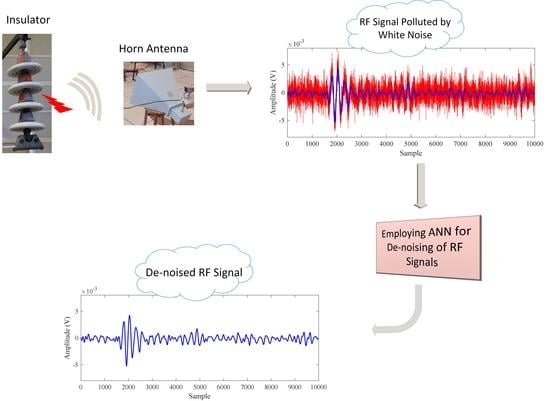
This paper presents a new method utilizing ANN curve fitting and function approximation abilities to remove white noise from RF PD signals. The method is proposed and compared with a WT based algorithm using different types of PD RF signals emitted from three damaged insulator discs, including ‘crack’, ‘internal void’, and ‘hardware sharp points’.
2. Laboratory Setup for PD Signals Measurement
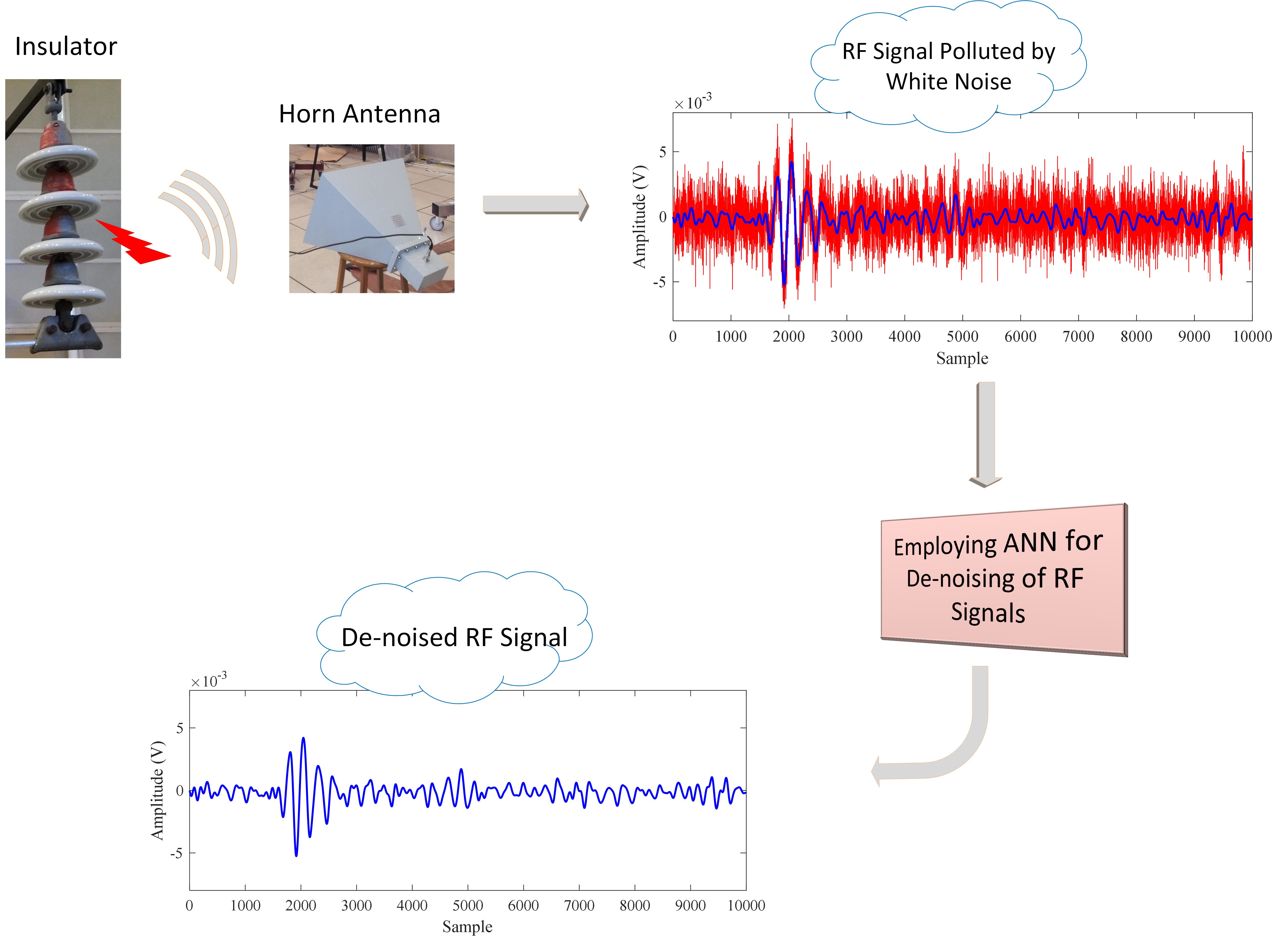
The ceramic insulators used as the samples consist of two different damaged insulator discs where the first disc is intentionally cracked, whereas the second sample has a hole in the disc cap [11]. Moreover, the corona is generated externally using sharp electrodes to mimic defects in overhead line hardware. The overall experimental setup is shown in Figure 1. PD was measured simultaneously using both RF antenna with 1–2 GHz bandwidth and classical PD measurement system. Each damaged disc is added to three intact discs in a string, then using a test transformer, 45 kVrms is applied to the strings; consequently, the wideband horn antenna captures the RF signals. The antenna is connected by a low impedance cable to a 2 GHz oscilloscope. Details of the setup are provided in [11].
3. Denoising of Partial Discharge RF Signals
The present section intends to discuss several parameters to quantify the severity of white noise. Also, both the wavelet transform and the proposed method are introduced.
3.1. Peak of Signal to Noise Ratio
In the process of PD signal examination, signal-to-noise ratio (SNR) is normally utilized in order to compare the energies of the original signal and white noise. However, it has been reported that for non-periodic transient signal calculating the peak signal-to-noise ratio (PSNR) is a better measure for the severity of white noise [12]. Therefore, being non-periodic and transient, RF signals better utilize the index of PSNR to assess the severity of white noise.
3.2. Factors for Evaluation of Denoising Algorithms
In terms of exploring and comparing the operation of denoising algorithms, the following parameters are exploited:
- The Electric Charge Error (QE):
- Root Mean Square Error (RMSE):
- Correlation Coefficient (CC):
- Signal-to-Noise Ratio—Denoised (SNRD):
where X, Y, and N represent the noise free PD current signal, the denoised RF signal, and the length of the measuring data window respectively.
3.3. Considering Discrete Wavelet Transform for Denoising of RF Signal
3.3.1. Basic Principles
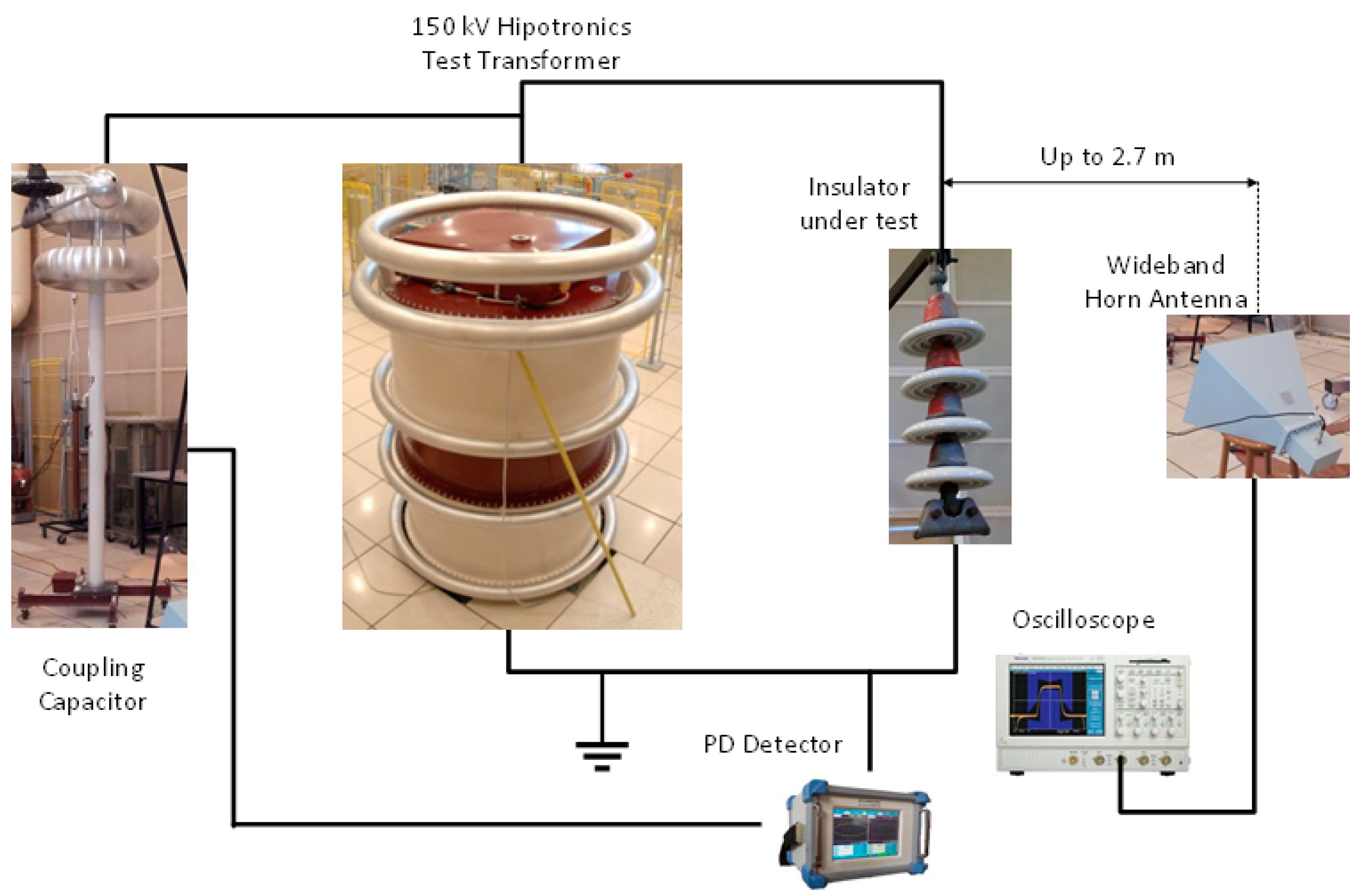
In this section, the process of the discrete wavelet transform (DWT) is highlighted and summarized in the following steps:
Step 1: In the first level of decomposition, the noisy signal Y(t) is applied to the high and low pass filters and coefficients of approximation (A1) and detail (D1) sub-bands are obtained. Afterward, in the second level of decomposition, the coefficients of A1, as a new signal, are applied to the new high and low pass filters. These processes are then continued to reach the desired pre-defined number of decomposition level (NDL), i.e., J.
Step 2: The thresholding procedure (TP) is used to remove the noise in the calculated coefficients of detail sub-bands (D1-J).
3.3.2. Mother Wavelet (MW) Selection
In the process of denoising by WT, the target is to keep the coefficients of the signal and noise suppression coefficients in the calculated sub-bands by TP. In the present paper, EBWS method is employed for MW selection, which has shown to give better results in the conducted simulations for denoising of RF signals. In EBWS, the distribution of signal energy in the sub-bands is utilized to select the best MW. In fact, a collection of appropriate MWs is considered; then an index, energy percentage (EP) achieved by (5), is calculated for all MWs. Next, in each level of decomposition, the MW corresponding with the biggest EP is selected as the optimum MW [14]. The selected MWs consist of Daubechies, orders 1–25 (db1–db25), symlets, orders 2–15 (sym2–sym15), and Coiflets, orders 1–5 (coif1–coif5).
where a, d, j, and k represent approximation coefficients, detailed coefficients, decomposition level, and length of samples in sub-bands, respectively. It should be noted that in most cases db4, as the MW, has presented better operation for denoising by WT exploited in this work.
3.3.3. Thresholding Procedure (TP)
As is discussed in the previous sub-section, TP must be implemented so that the components of the signal and the noise elements are maintained and eliminated in the detail sub-bands, respectively. Thus, the performance of signal denoising by WT is depended on the way of threshold value calculation. In this paper, the proposed idea by [10], energy conservation-based method (ECBT), considered as one of the promising methods, is implemented as follows:
- The original noise-free signal is decomposed to reach the predefined level, J, resulting in AJ and D1-J sub-bands.
- The mentioned procedure above is repeated for the noisy signal, in order to achieve NAJ and ND1-J sub-bands as well.
- The coefficients of NAJ are kept completely, and all components of ND1 are set on zero. Next, threshold values, λJ, are estimated for each level of ND2-J, and the coefficients are then thresholded using (6)
where, X and λj, respectively, present the coefficients and threshold value of level j, obtained by (7).
where Aj, nj, EDj, and ENDj are the vector obtained through (8), the length of NDj, energy of the detail sub-band Dj, and energy of the noisy detail sub-band NDj, respectively.
Since the original noise-free signal is not available to attain EDj, a pre-defined lookup table is proposed by authors [10], demonstrating the necessity of a prior knowledge of PD signals for implementation of ECBT.
3.4. Proposed Method
The proposed idea in this section introduces a novel approach to the problem of denoising, employing ANN. In fact, the process of denoising in this algorithm is merely carried out in time-domain instead of currently widespread time–frequency domain algorithms. In other words, the samples of the digital signal are considered as a collection of discrete ones, rather than a continuous signal, intended to be fitted by an appropriate curve and is explained in the present subsections.
3.4.1. Artificial Neural Network Curve Fitting
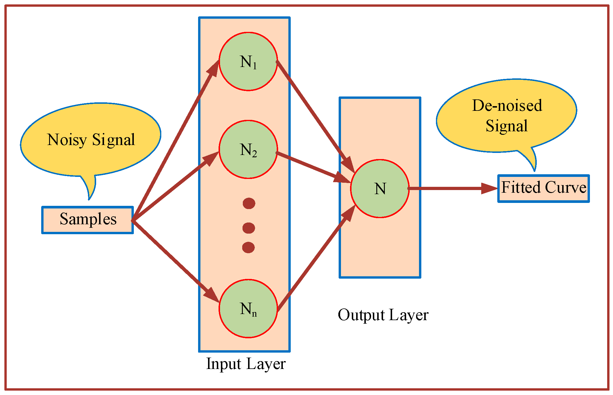
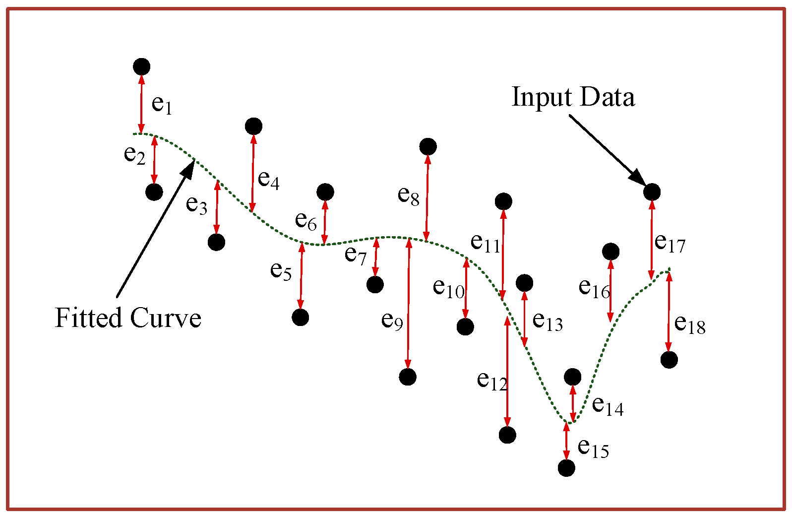
Artificial neural network is a prevalent algorithm exploited in curve fitting, data classification, and time-series problems [15]. In this work, a multi-layer perceptron network is employed in which the samples of the measured noisy signal are assumed as the inputs and the output is the fitted curve, as depicted in Figure 3. The structure of the employed ANN includes a feed-forward network, in the input and output layers, comprised of sigmoid and linear activation functions, respectively. As shown in Figure 4, a series of samples, which are the ANN input vector, is approximated using an appropriate curve and the output of ANN corresponds to the least square error and obtained by Equation (9). Thus, the acquired curve in the process is considered as the denoised signal.
where n and ei are assumed to be the number of the samples and the error of the ith sample, respectively.
3.4.2. Suitable Number of Neurons for the Structure of the ANN
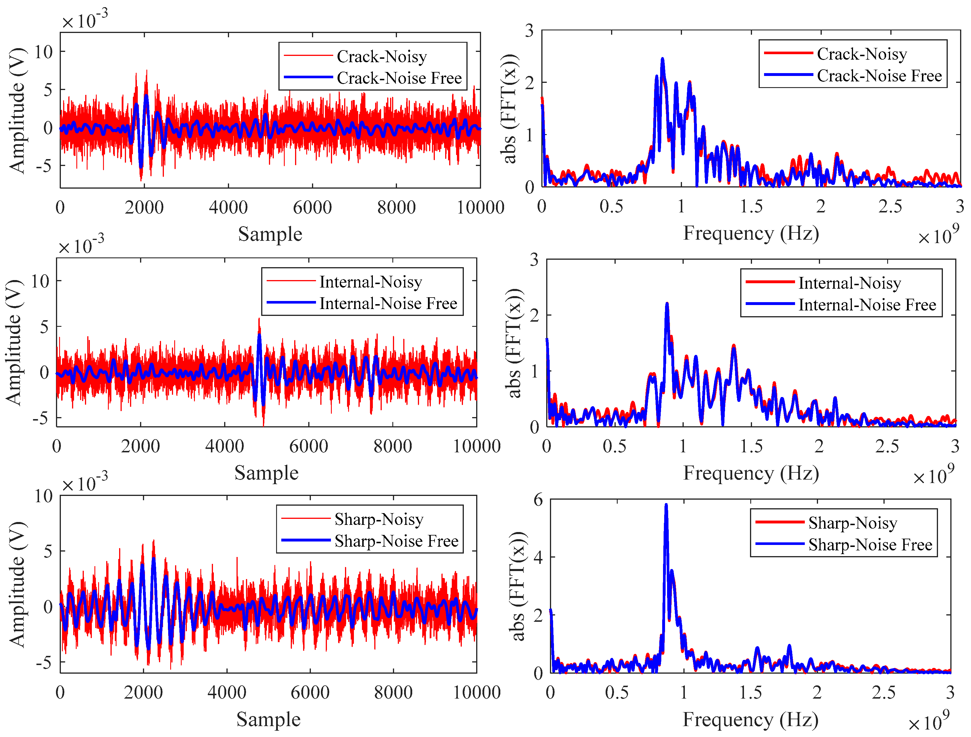
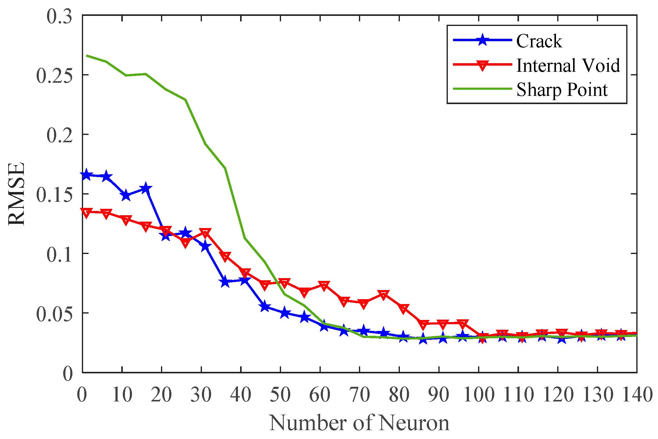
In this paper, a two-layer ANN is considered to avoid the computational burden of higher layers of ANN. Hence, while the output layer is made up by one neroun, the first layer is going to be investigated in this subsection. Therefore, to attain a suitable number of neurons for the first layer, different values will be examined for three types of the RF signals and the one that results in the least RMSE will be selected, shown in Figure 5. It should be noted that in this figure the signals and their frequency spectrum both in noise-free and noisy condition (PSNR = 1) are depicted. It is worth mentioning that the optimization method, exploited in this investigation, is Levenberg–Marquardt. As shown in Figure 6, 100 neurons showed the lowest RMSE for the three different measured RF signals. It should be noted that the length of the data window (DW) is 10,000 samples and it is assumed as a basic data window (BDW) in the paper. Therefore, longer DWs are considered the main data window (MDW) and hence must be divided into the BDWs.
3.4.3. Optimization Methods
In this subsection, the performance of five optimization methods, including Levenberg–Marquardt, Bayesian regularization, BFGS quasi-Newton, resilient back-propagation, and scaled conjugate gradient for the utilized ANN in the proposed method is investigated. Hence, the operation of these functions for denoising of the RF signal, for instance, the sharp point type, in three noise levels are explored and shown in Table 1. As seen, in all cases, the best performance is obtained by Levenberg–Marquardt; therefore, it is exploited in the structure of ANN in the proposed method as the best optimization method.
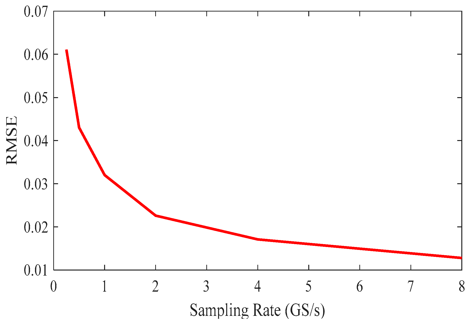
3.4.4. Effect of Sampling Rate on the Performance of the Proposed Method
In this subsection, the performance of the proposed method is considered from the sampling rate effect point of view. Hence, the RF signal, for the PD source of a sharp point, in the cases of different sampling rate is exploited in this investigation. Therefore, denoising of the signal in each case is carried out and the factor RMSE is calculated for each, shown in Figure 7. As seen, the more sampling rate for RF signal, the more accuracy in the denoising procedure by the proposed method can be obtained, where the lowest error is observed for the signal by 8 GS/s. However, in this work, the sampling rate of 2 GS/s is used for PD signal measuring, due to the computational burden.
3.4.5. Full Procedure of the Proposed Method
The proposed method can be summarized as follows:
- Normalizing the RF signal bywhere X and XN are the main RF signal and normalized one, respectively.
- Dividing MDW into the pre-defined BDW with 10,000 samples lengths each.
- Separately denoising each BDW, using 100 neurons in the ANN structure.
- Connecting all BDWs together to attain the complete denoised MDW RF signal.
- Obtaining the real RF signal by multiplying the maximum value, achieved in Step 1, by the signal denoised in Step 4.
4. Results and Discussions
4.1. Effectiveness of the Proposed ANN-Based Denoisng Technique
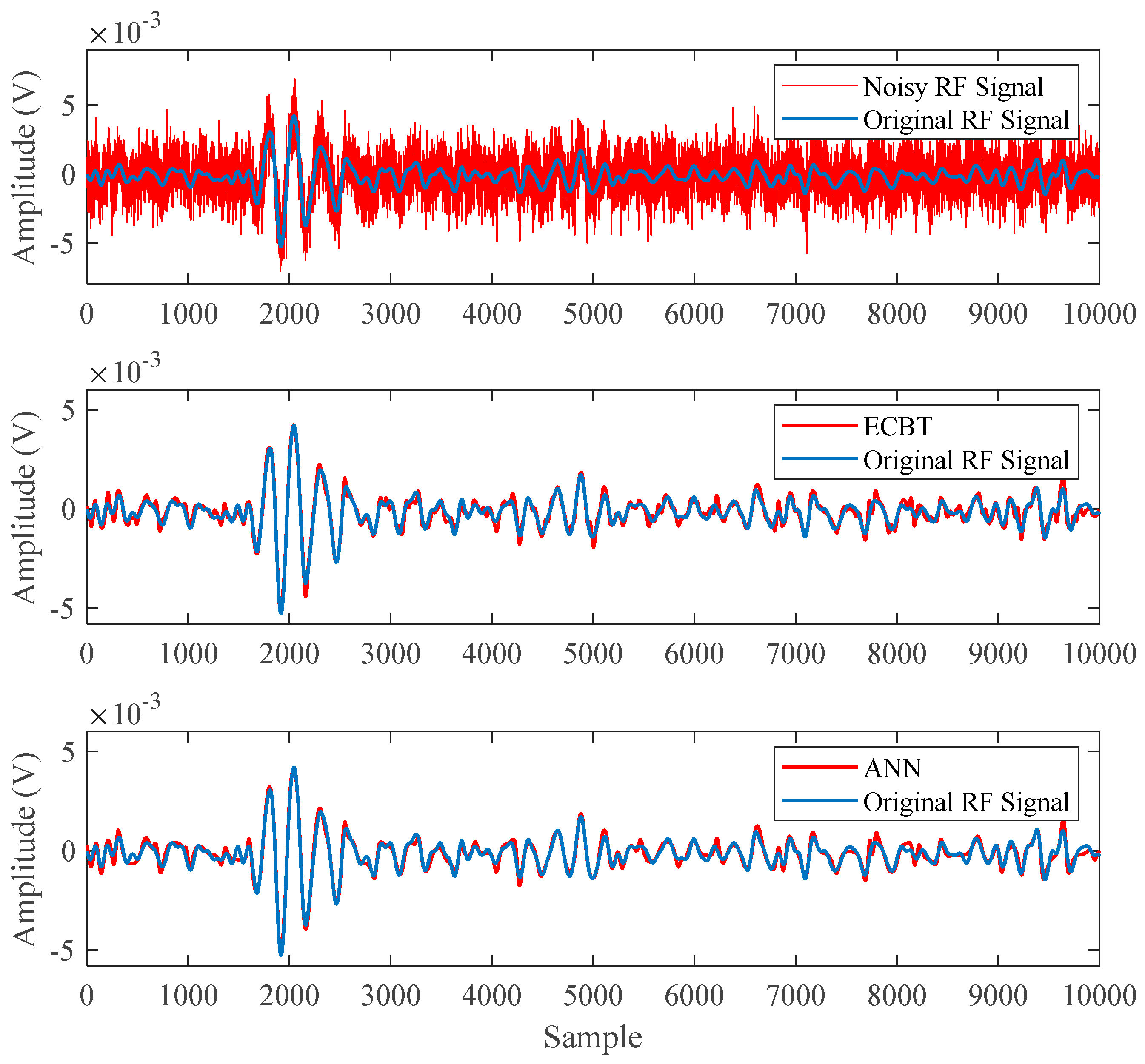
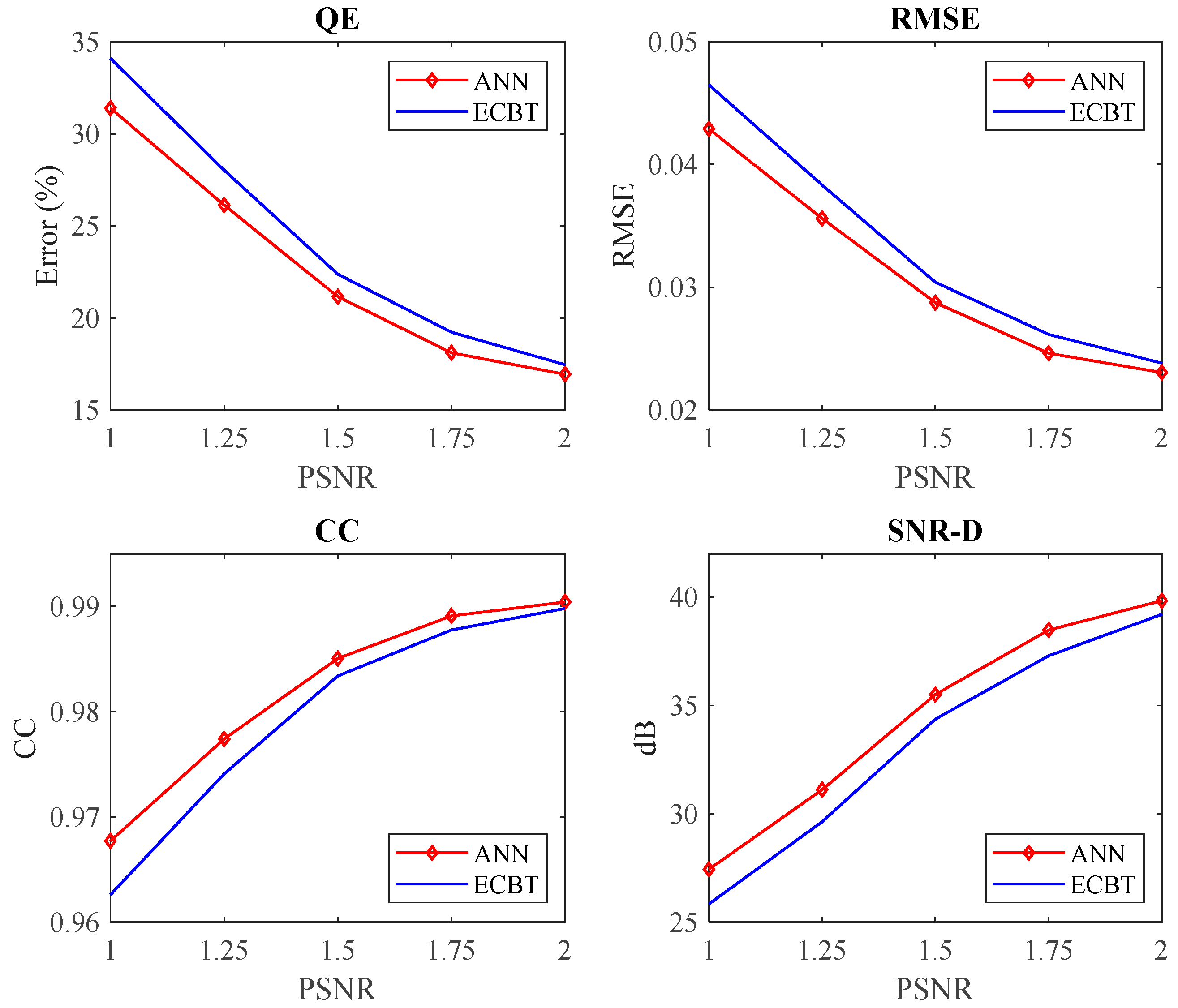
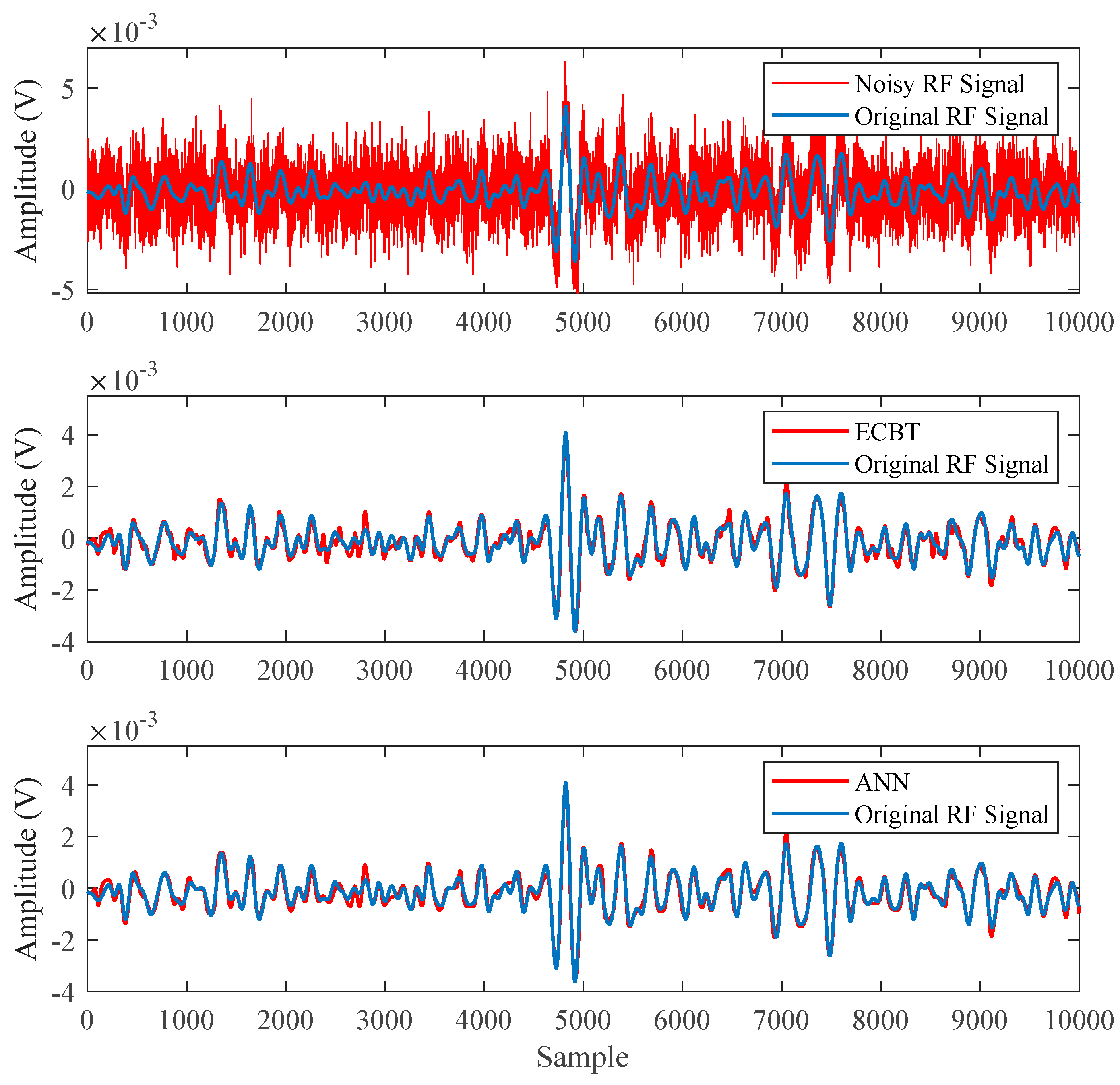
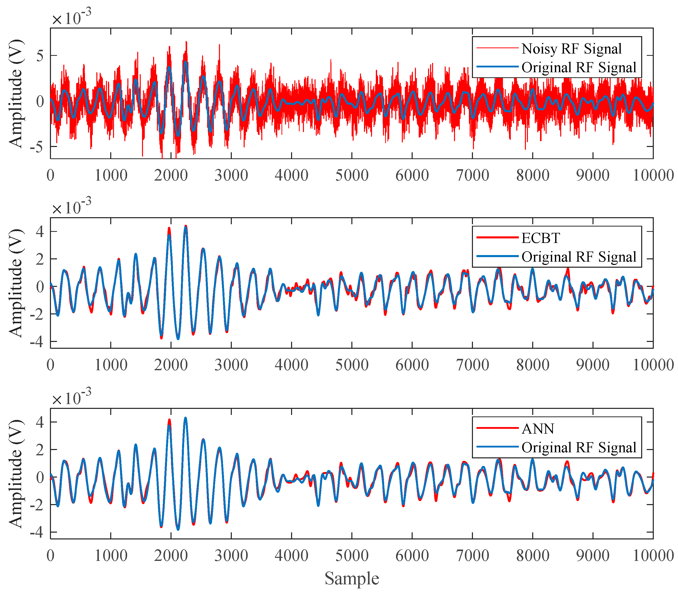
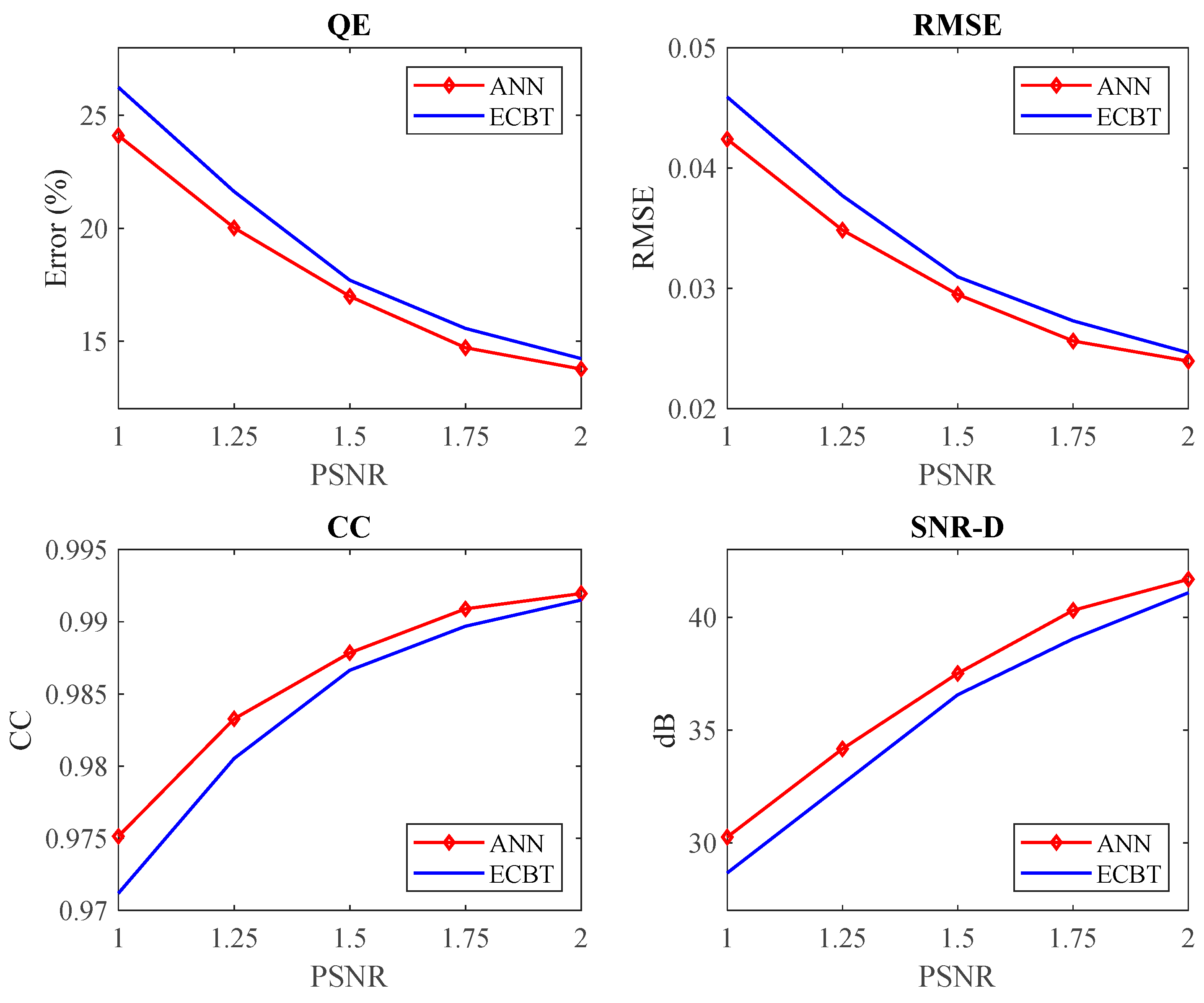
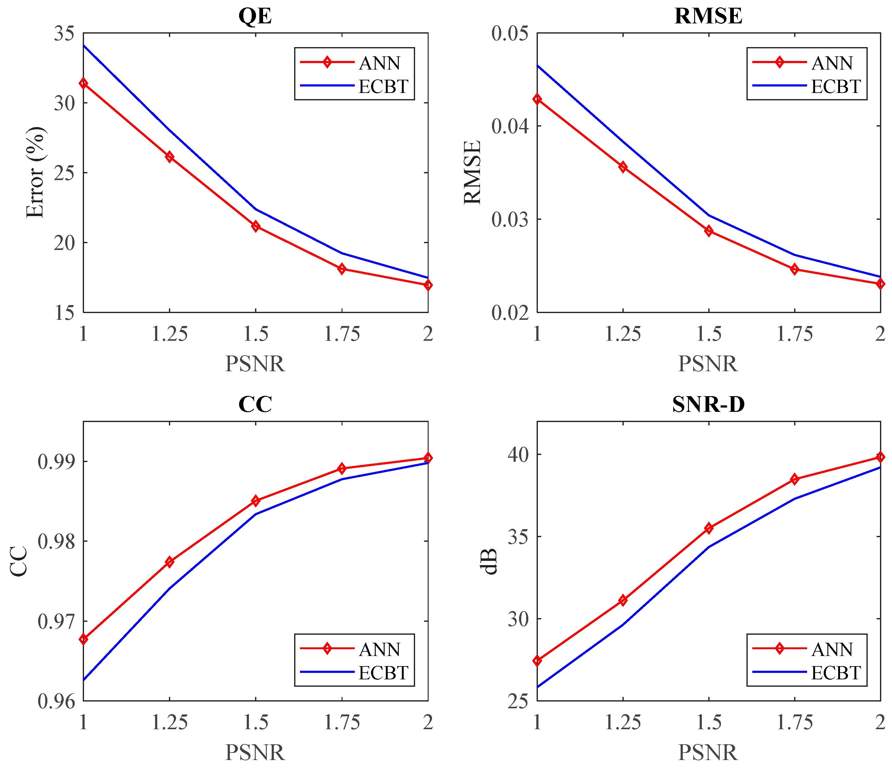
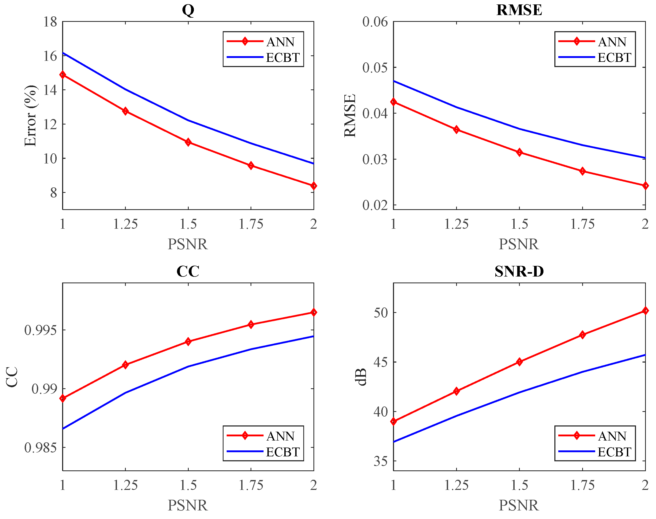
In this section, the RF signals are polluted with white noise at different levels, with PSNR ranging from 1 to 2 with steps of 0.25. Moreover, the obtained results from denoising with the proposed method as well as the wavelet-based method are presented. In Figure 8, the result for the first type of RF signal generated from a crack for a severe noise (PSNR = 1) is shown. Additionally, the denoising evaluation factors—including QE, RMSE, CC, and SNRD—are exploited in order to compare the proposed method with ECBT in the different values of PSNR, as depicted in Figure 9. It is evident that ANN-based denoising technique showed a better performance than ECBT in all calculated parameters. These investigations are repeated for other RF signals, namely internal void, and sharp point types, as well; hence, denoising results for the most severe noise are, respectively, depicted in Figure 10 and Figure 11 for the named damaged types mentioned above. In addition, the proposed method is compared with ECBT in cases of various PSNR, for both RF signals including internal void and sharp point types, as shown in Figure 12 and Figure 13, respectively. As depicted, the proposed method demonstrates its superiority in RF signal denoising.
It is noteworthy that, in ECBT, the proposed method by authors in [10], exploitation of a pre-defined lookup table in the process of denoising is imperative, due to the fact that there is no noise-free original signal for the implementation of the method in the real situation. Whereas, in this work, the noise-free RF signals are exploited instead of using the pre-defined lookup table. That means the proposed method is compared to ECBT with the highest possible performance, being probably too optimistic. Additionally, there is no idea about the optimum number of decomposition levels for DWT, likely to vary for each PD signal. Here, we performed denoising with ECBT in various decomposition levels, including 1 to 8 levels and the optimum results are obtained for the case of 5 levels, utilized in ECBT for denoising of these RF signals.
4.2. Consideration of Denoising for Combining Two RF Signals
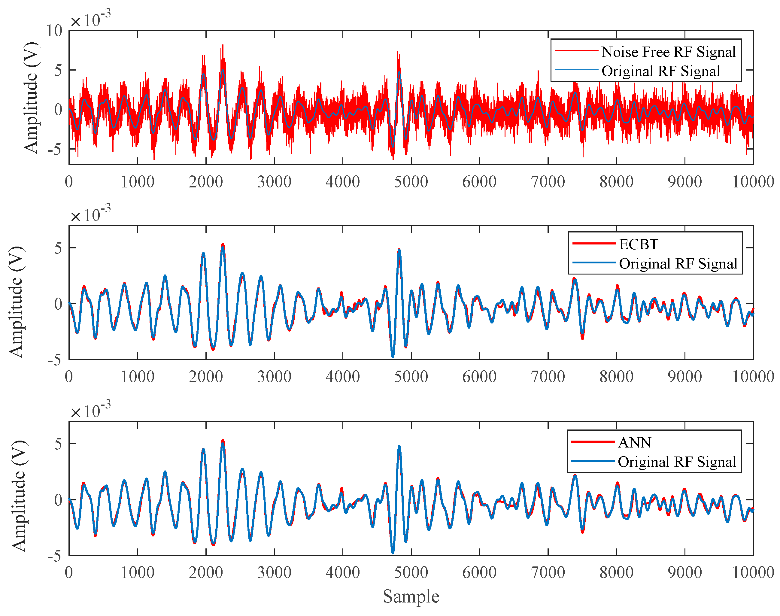
This subsection seeks to consider the performance of the denoising methods in the case of a combination of two RF signals. In fact, it is assumed that in the process of PD signals measuring, two PD sources generate RF signals, simultaneously, and the horn antenna captures both. Thus, the measured signal, for instance, the combination of ‘sharp’ and ‘internal’ types, are utilized for comparing the proposed method and ECBT in various noise levels. Hence, the denoising results for severe noises (PSNR = 1) are shown in Figure 14 and the comparison in various noise level is given in Figure 15.
5. Conclusions
In this paper, an ANN-based approach is introduced for white noise suppression. The paper investigates the influence of the main ANN parameters on the performance of the proposed method, namely the appropriate number of neurons and the optimization method for the structure of ANN. Moreover, WT-based algorithm called ECBT is used for comparison, as one of the most popular algorithms for PD signal denoising. The performance of the proposed method is examined by the laboratory-measured RF signals emitted from different PD sources, namely crack, internal void, and hardware sharp points. The RF signals are contaminated with white noise at various levels, with the PSNR ranging from 1 to 2 with the step of 0.25. In all tested cases, the evaluation factors prove a significant superiority of the proposed method for denoising of PD RF signals compared to ECBT. In addition to the ANN superior performance, it is noteworthy that using WT-based algorithms still suffers from other restrictions like mother wavelet selection, determination of the number of decomposition levels, and thresholding procedure. Moreover, to get high performance of WT-based methods, prior knowledge of the signal is needed; whereas, the proposed method is implemented simply without exploiting any prior knowledge.
Author Contributions
Conceptualization, A.A.S. and A.E.-H.; methodology, A.A.S.; software, A.A.S.; validation, A.A.S.; formal analysis, A.A.S.; investigation, A.A.S. and A.E.-H.; resources, A.A.S. and A.E.-H.; data curation, A.E.-H.; writing—original draft preparation, A.A.S.; writing—review and editing, A.E.-H.; visualization, A.A.S. and A.E.-H.; supervision, A.E.-H.; project administration, A.E.-H.
Funding
This research received no external funding.
Conflicts of Interest
The authors declare no conflicts of interest.
References
- Hussein, R.; Shaban, K.B.; El-Hag, A. Denoising different types of acoustic partial discharge signals using power spectral subtraction. High Volt. 2018, 1, 44–50. [Google Scholar] [CrossRef]
- Ghorat, M.; Gharehpetian, G.B.; Latifi, H.; Hejazi, M.A. A new partial discharge signal denoising algorithm based on adaptive dual-tree complex wavelet transform. IEEE Trans. Inst. Meas. 2018, 67, 2262–2272. [Google Scholar] [CrossRef]
- Carvalho, A.T.; Lima, A.C.S.; Cunha, C.F.F.C.; Petraglia, M. Identification of partial discharges immersed in noise in large hydro-generators based on improved wavelet selection methods. Measurement 2015, 75, 122–133. [Google Scholar] [CrossRef]
- Kopf, U.; Feser, K. Rejection of narrow-band noise and repetitive pulses in on-site PD measurements. IEEE Trans. Dielectr. Electr. Insul. 1995, 6, 1180–1191. [Google Scholar] [CrossRef]
- Sriram, S.; Nitin, S.; Prabhu, K.; Bastiaans, M. Signal denoising techniques for partial discharge measurements. IEEE Trans. Dielectr. Electr. Insul. 2005, 12, 1182–1191. [Google Scholar] [CrossRef]
- Ashtiani, M.B.; Shahrtash, S.M. Feature-oriented denoising of partial discharge signals employing mathematical morphology filters. IEEE Trans. Dielectr. Electr. Insul. 2012, 19, 2128–2136. [Google Scholar] [CrossRef]
- Soltani, A.A.; Shahrtash, S.M. Self-adaptive morphological filter for noise reduction of partial discharge signals. In Proceedings of the 33rd Power System Conference, Tehran, Iran, 22–24 October 2018. [Google Scholar]
- Wu, Z.; Huang, N.E. Ensemble empirical mode decomposition: A noise-assisted data analysis method. Adv. Adapt. Data Anal. 2009, 1, 1–41. [Google Scholar] [CrossRef]
- Jin, T.; Li, Q.; Mohamed, A.M. A novel adaptive EEMD method for switchgear partial discharge signal denoising. IEEE Access 2019, 7, 58139–58147. [Google Scholar] [CrossRef]
- Hussein, R.; Shaban, K.B.; El-Hag, A. Energy conservation based thresholding for effective wavelet denoising of partial discharge signals. IET Sci. Meas. Technol. 2016, 10, 813–822. [Google Scholar] [CrossRef]
- Anjum, S.; Jayaram, S.; El-Hag, A.; Jahromi, A.N. Detection and classification of defects in ceramic insulators using RF antenna. IEEE Trans. Dielectr. Electr. Insul. 2017, 24, 183–190. [Google Scholar] [CrossRef]
- Najafipour, A.; Babaee, A.; Shahrtash, S.M. Comparing the trustworthiness of signal-to-noise ratio and peak signal-to-noise ratio in processing noisy partial discharge signals. IET Sci. Meas. Technol. 2012, 7, 112–118. [Google Scholar] [CrossRef]
- Mortazavi, S.; Shahrtash, S. Comparing denoising performance of DWT, WPT, SWT AND DT-CWT for partial discharge signals. In Proceedings of the 43rd International Universities Power Engineering Conference, Padova, Italy, 1–4 September 2008. [Google Scholar]
- Li, J.; Jiang, T.; Grzybowski, S.; Cheng, C. Scale dependent wavelet selection for denoising of partial discharge detection. IEEE Trans. Dielectr. Electr. Insul. 2010, 17, 126–137. [Google Scholar] [CrossRef]
- Budiman, F.N.; Khan, Y.; Malik, N.H.; Al-Arainy, A.A.; Beroual, A. Utilization of artificial neural network for the estimation of size and position of metallic particle adhering to spacer in GIS. IEEE Trans. Dielectr. Electr. Insul. 2013, 20, 2143–2151. [Google Scholar] [CrossRef]
Figure 1.
Laboratory setup for simultaneous electrical and RF signals measurement from the source of partial discharge, defected insulator disc.
Figure 1.
Laboratory setup for simultaneous electrical and RF signals measurement from the source of partial discharge, defected insulator disc.

Figure 2.
The schematic diagram of the process of denoising by wavelet transform, including decomposition with DWT, thresholding, and inverse DWT.
Figure 2.
The schematic diagram of the process of denoising by wavelet transform, including decomposition with DWT, thresholding, and inverse DWT.

Figure 3.
Structure of the ANN in the proposed method.

Figure 4.
Curve fitting in the procedure of optimization by ANN to achieve the least square error.

Figure 5.
Three RF signals emitted from the different sources of partial discharge in the insulator discs including crack, internal void, and sharp point types and their frequency spectrum both in noisy and noise free conditions.
Figure 5.
Three RF signals emitted from the different sources of partial discharge in the insulator discs including crack, internal void, and sharp point types and their frequency spectrum both in noisy and noise free conditions.

Figure 6.
Considering the suitable number of neurons for the three different RF signals.

Figure 7.
Results of denoising, the factor RMSE, in the various sampling rates of RF signals.

Figure 8.
Denoising of RF signal, ‘crack’ type, in the case of PSNR = 1.

Figure 9.
Results of denoising from RF signal in different noise levels where PSNR ranges from 1 to 2 by steps of 0.25, in the case of ‘crack’ type.
Figure 9.
Results of denoising from RF signal in different noise levels where PSNR ranges from 1 to 2 by steps of 0.25, in the case of ‘crack’ type.

Figure 10.
Denoising of RF signal, ‘internal void’ type, in the case of PSNR = 1.

Figure 11.
Denoising of RF signal, ‘sharp point’ type, in the case of PSNR = 1.

Figure 12.
Results of denoising from RF signal in different noise levels where PSNR ranges from 1 to 2 by steps of 0.25, in the case of ‘internal void’ type.
Figure 12.
Results of denoising from RF signal in different noise levels where PSNR ranges from 1 to 2 by steps of 0.25, in the case of ‘internal void’ type.

Figure 13.
Results of denoising from RF signal in different noise levels where PSNR ranges from 1 to 2 by steps of 0.25, in the case of ‘sharp point’ type.
Figure 13.
Results of denoising from RF signal in different noise levels where PSNR ranges from 1 to 2 by steps of 0.25, in the case of ‘sharp point’ type.

Figure 14.
Denoising of RF signal, combination of ‘sharp point’ and ‘internal void’ types, PSNR = 1.
Figure 14.
Denoising of RF signal, combination of ‘sharp point’ and ‘internal void’ types, PSNR = 1.

Figure 15.
Results of denoising from RF signal in different noise levels where PSNR ranges from 1 to 2 by steps of 0.25, in the case of combination of ‘sharp point’ and ‘internal void’ types.
Figure 15.
Results of denoising from RF signal in different noise levels where PSNR ranges from 1 to 2 by steps of 0.25, in the case of combination of ‘sharp point’ and ‘internal void’ types.


Table 1.
The results of denoising, the factor RMSE, by five optimization methods and in the cases of three levels of noise (PSNR) including 1, 1.5, and 2
Table 1.
The results of denoising, the factor RMSE, by five optimization methods and in the cases of three levels of noise (PSNR) including 1, 1.5, and 2
| Optimization Method | PSNR | ||
|---|---|---|---|
| 1 | 1.5 | 2 | |
| Levenberg–Marquardt | 0.04102 | 0.02899 | 0.02258 |
| Bayesian Regularization | 0.04387 | 0.02966 | 0.02263 |
| BFGS Quasi-Newton | 0.04236 | 0.03041 | 0.02261 |
| Resilient Back Propagation | 0.04296 | 0.02918 | 0.02283 |
| Scaled Conjugate Gradient | 0.04165 | 0.03039 | 0.02276 |
© 2019 by the authors. Licensee MDPI, Basel, Switzerland. This article is an open access article distributed under the terms and conditions of the Creative Commons Attribution (CC BY) license (http://creativecommons.org/licenses/by/4.0/).
Share and Cite
MDPI and ACS Style
Soltani, A.A.; El-Hag, A. Denoising of Radio Frequency Partial Discharge Signals Using Artificial Neural Network. Energies 2019, 12, 3485. https://doi.org/10.3390/en12183485
AMA Style
Soltani AA, El-Hag A. Denoising of Radio Frequency Partial Discharge Signals Using Artificial Neural Network. Energies. 2019; 12(18):3485. https://doi.org/10.3390/en12183485
Chicago/Turabian StyleSoltani, Amir Abbas, and Ayman El-Hag. 2019. "Denoising of Radio Frequency Partial Discharge Signals Using Artificial Neural Network" Energies 12, no. 18: 3485. https://doi.org/10.3390/en12183485
Note that from the first issue of 2016, this journal uses article numbers instead of page numbers. See further details here.