A Workflow for Optimization of Flow Control Devices in SAGD

1
School of Mining & Petroleum Engineering Department of Civil & Environmental Engineering, University of Alberta, Edmonton, AB T6H 1G9, Canada
2
Department of Geoscience, University of Calgary, Calgary, AB T2N 1N4, Canada
*
Author to whom correspondence should be addressed.
Energies 2019, 12(17), 3237; https://doi.org/10.3390/en12173237
Submission received: 8 July 2019
/
Revised: 15 August 2019
/
Accepted: 19 August 2019
/
Published: 22 August 2019
(This article belongs to the Special Issue Reservoir Simulation and Prediction of Gas, Oil and Coal Mine)
Abstract
:In McMurray Formation, steam assisted gravity drainage is used as the primary in-situ recovery technique to recover oil sands. Different geological reservoir settings and long horizontal wells impose limitations and operational challenges on the implementation of steam-assisted gravity drainage (SAGD). The dual-string tubing system is the conventional completion scheme in SAGD. In complex reservoirs where dual-string completion cannot improve the operation performance, operators have adopted flow control devices (FCDs) to improve project economics. FCDs secure more injection/production points along the horizontal sections of the SAGD well pairs, hence, they maximize ultimate bitumen recovery and minimize cumulative steam-oil ratio (cSOR). This paper will focus on the optimization of outflow control devices (OCDs) in SAGD reservoirs with horizontal wellbore undulations. We present the detailed optimization workflow and show the optimization results for various scenarios with well pair trajectory undulation. Comparing the results of the optimized OCDs case with a dual-string case of the same SAGD model shows improvements in steam distribution, steam chamber growth, bitumen production, and net present value (NPV).
1. Introduction
The Canadian oil sands found in the prairie province of Alberta have over 165 billion barrels of oil (Alberta’s Energy Reserves and Supply/Demand Outlook Report 2017), ranking Canada as the third largest country in oil reserves in the world. The extremely viscous nature of the bitumen makes it a challenging issue to unlock those proven reserves and bring them to surface. Besides open-pit mining that contributes to only 10% of the total recovery, steam-assisted gravity drainage (SAGD) has been adopted and developed as an in-situ recovery technique for bitumen production [1].
In SAGD operations, the dual-tubing-string system is the conventional well completion scheme. The well pairs are completed with a short tubing landed at the heel section of the well, and a long tubing is extended all the way to the toe. This completion design offers two injection points in the well and leads to a better steam chamber development along the horizontal well compared to a single point production and injection. The dual tubing completion, however, leads to a non-uniform steam chamber growth, owing to factors such as the reservoir heterogeneity and variations in the reservoir structure [2,3,4].
Additional factors that impact the overall SAGD performance include wellbore undulations (i.e., undesired deviations in well pair trajectories that have been unintentionally generated during drilling operations), bottom and top water, top gas, point bar deposits that contain inclined heterolithic stratification (IHS), mud drapes, vertical permeability baffles, abandoned mud channels and regional low reservoir ceiling [5,6]. The direct impact of these factors is heat losses to the cap rock and a waste of steam energy that is reflected in low bitumen recovery efficiency and a higher cumulative steam-oil ratio (cSOR), leading to suboptimal project economics.
In SAGD operations, flow control devices (FCDs) offer great flexibility in controlling the injection and production operations along the horizontal wells. Some SAGD operators have adopted FCDs to improve project economics, maximizing the ultimate bitumen recovery, and minimizing the cSOR [7]. A variety of FCDs are commercially available in the oil and gas industry [8]. The devices have been successfully used in the conventional reservoirs for several years to control water and gas breakthrough [9]. The application of FCDs in SAGD well design is relatively new.
ConocoPhillips’s first use of FCDs was in Surmont field SAGD project in 2009 [2]. Suncor implemented its first FCDs pilot in Suncor’s MacKay River project in 2011 [10]. Further examples include Cenovus Pelican Lake in 2012, Husky Tucker in 2011 and 2012, Devon Jackfish in 2011, Nexen Long Lake in 2013, and Shell Orion in 2012 [11].
A few researchers have focused on optimizing FCDs design and design parameters. Sidahmed et al. [12] have presented details about the construction of the wellbore-reservoir simulation model and performed grid size sensitivity analysis and implemented local grid refinement to improve simulation accuracy in FCDs design optimization. Kyanpour and Chen (2014) [6], also used coupled wellbore-reservoir simulation to determine optimum size and position of FCDs in heterogeneous reservoirs. Nejadi et al. [5], incorporated geological details of meander belt deposits in their simulations and utilized the trust region algorithm for optimal FCDs placement.
This paper presents a workflow to optimize the placement and number of ports of outflow control devices (OCDs). The main objective is to overcome the deficiencies brought about by wellbore undulations on SAGD performance. The analysis deploys a coupled wellbore-reservoir simulation model where CMG’s FlexWell for wellbore hydraulics modeling is linked with CMG-STARS for thermal reservoir simulations. CMOST toolbox is utilized in the optimization workflow.
2. Optimization Workflow
The optimization steps follow an optimization workflow as shown in Figure 1.
The simplified net present value (NPV) objective function shown in Equation (1) is implemented and linked to the optimization algorithm. The equation provides NPV estimates for different solutions during the optimization process.
where Qo is oil production rate, Qw is steam injection rate, ro is oil price, rw is steam cost, tref is reference time, and Tp is the project life time.
The objective function in Equation (1) is a simplified version of a more detailed equation that accounts for fixed capital expenses, including the cost of installed OCDs, which is assumed to be negligible in the research work of this paper [13]. In the calculations, the oil price is assumed to be $50 per barrel, steam cost is assumed to be $8/bbl cold water equivalent (CWE), and discount factor (D) is assumed to be 0.1 per year.
The SAGD models were allowed to continue until the daily increment of the NPV became zero; i.e., (ΔNPV/Δt = 0). The NPV function formula is designed to perform automatic termination of the SAGD process when daily incremental NPV of the project becomes nil.
Details of this optimization workflow are discussed next.
2.1. Optimization Parameters
It is essential to set reasonable ranges for optimization parameters because of limited computational resources and time, and because the parameters involved in the optimization work are highly non-linear. For the work in this paper, the aim is to optimize OCD’s number of ports for each OCD in the range 0–70 with a fixed increment of five. Hence, the total number of optimization variables is 60. The optimization study in this paper involves over 50,000 possible combinations (154 = 50,625 cases). However, this enormous number of possible combinations imposes the need for an automatic optimization tool.
Restriction-style OCDs (e.g., orifice type) were adopted throughout this paper. The maximum number of OCDs per well in the optimization work in this paper is set at four. However, this number can be reduced depending on the optimization results.
Generally, the number and size of OCD ports (orifice diameter) vary from one manufacturer to another, and standard port sizes of inflow control devices (ICDs) are usually less than those for OCDs. In this paper, a typical OCD port size of 10 mm is used [7,14,15]. Additionally, the maximum number of ports per single OCD is assumed to be 70 ports with fixed increments of five; i.e., (5, 10, 15, etc.). When the optimized number of ports is high, several OCD joints can be used in a row (with every single joint having a maximum of 35 ports).
This study assumes that the toe of long-tubing strings is fully open to the flow. Table 1 summarizes all fixed parameters of the optimization workflow.
2.2. Optimization Tool
The default optimization engine that has been adopted in the optimization work of this paper is the CMG CMOST DECE engine. The term DECE stands for designed exploration and controlled evolution.
A DECE is a two-stage iterative optimizer. In the first stage (designed exploration), the optimizer explores the parameter space and gathers the maximum amount of information about the solution space. Using experimental design techniques, the algorithm rejects and prevents poor performance candidates from being used in the next designed exploration stage. Estimated NPV is the criterion to select and promote candidate models. Controlled evolution algorithm is further applied in the second stage. Candidate values of each parameter (number of ports in each FCD in our case) are examined for a better chance to improve the possible solution quality.
To minimize the risk of getting trapped in local optima, the DECE algorithm keeps an eye on banned candidate values and examines them on a regular basis to check whether the banned decision is still valid or not. If the banned decision is valid, banned candidate values will stay banned. If not, those banned candidate values will be recalled and utilized in the exploration stage again.
2.3. Design of Experiments
We consider the input model parameters as random variables and model the uncertainty about the values. The forward model, which is the reservoir simulator, transforms the inputs with a known probability distribution. In the case of SAGD optimization, the transformation function solves the multiphase fluid flow in porous media and consists of mass, momentum, and the energy conservation equation. The problem is solved using finite difference, and it incurs huge computation costs to the optimization problem. We implemented the design of experiments in the first stage of optimization to explore the solution space and filter out proposals with poor performance.
Several algorithms are available in the literature for parameter sampling and design of experiments [16]. We implemented Latin hypercube sampling (LHS) in our optimization workflow as it explores the complete parameters space with limited number of points. Unlike Monte Carlo sampling, in which the samples are independent from each other, LHS partitions the probability distribution into intervals of equal probability and spreads the samples more evenly across the probability density function.
Dealing with more than 50,000 possible optimum cases during the optimization study makes it difficult to pick the optimum case by running only 500 cases out of those 50,000 cases (less than 1% of total possible cases). Although the CMOST DECE optimization tool is reliable in picking the optimum case out of those 50,000 possible optimum cases, running some preselected cases prior to automatic generation of possible optimum cases using the optimization tool helps in exploring the possible optimum cases and improving chances of determining the search direction to be followed by the optimization tool. The process of selecting those exploratory cases is called “design experimental sampling”. The term “experimental” refers to a single simulation case that has been created based on selected sample values for each parameter; the selected set of experiments is called “design,” and “sampling” simply means selection; and it is done with a known design space that depends on parameters (number of OCD’s) and sample values (number of ports).
2.3.1. Short-Term Optimization
All simulation cases during this step are run for a short period (three years) of project life time, which represents the early-stage SAGD performance. This step aims at optimizing the number of ports in each of the installed OCDs in relatively fast simulations. We examined the performance of 500 cases over three years. The proposals are ranked based on the calculated NPV. Cases with the highest NPV are accepted for the full SAGD project life and are analyzed in the next step.
Setting the lower bound for the number of ports at zero allows optimizing the locations and number of required OCDs within the maximum considered number. If there is unnecessary OCD at a specific location, its number of ports will converge to zero or a small number.
2.3.2. Long-Term Optimization
After ranking the short-term simulation results, the simulation durations of the top 50 cases are extended and allowed to run until the end of the SAGD project life. The case that yields the highest NPV is considered to be the optimum case; i.e., the case with the optimum locations, and the number of ports for OCDs. Table 2 shows Optimization steps one and two.
3. Case Study
3.1. Dynamic Reservoir Model
The 3D model dimensions were set based on average dimensions of a typical SAGD well pair-length and operating volume dimensions in the MacKay River project [10]. The model has a length of 1000 m along the horizontal well pair directions (J-direction), a width of 34 m (I-direction) and a height of 30 m (K-direction). The model was discretized into 10,200 grid blocks. The horizontal length in J-direction was divided into 20 blocks with each grid block having a length of 50 m. The grid blocks, which are connected to the injection and production wells, were divided into smaller grid blocks using local grid refinement (LGR). The 34 m in I-direction was divided into 17 grid blocks with each grid block having 2-m length. The 30 m in K-direction was divided into 30 grid blocks with each grid block having 1-m length. Sidahmed (2018) [13] performed a grid size sensitivity analysis and proposed the optimal grid sizes for SAGD simulation, considering both simulation run time, and accuracy.
The reservoir model is constructed from the MacKay River SAGD project located approximately 60 km northwest of the city of Fort McMurray, AB, Canada. Table 3 shows the average reservoir properties used in the model. Constant reservoir rock properties, together with orthogonal simulation grids, greatly improves the simulation runtime, which is favorable for parameter optimization. Being a trade-off, it affects the geological realism of the model and simulation accuracy. Including detailed geology of the point bar deposits of the Lower Cretaceous McMurray Formation reduces the uncertainties and improves the predictive capabilities of modeling [5].
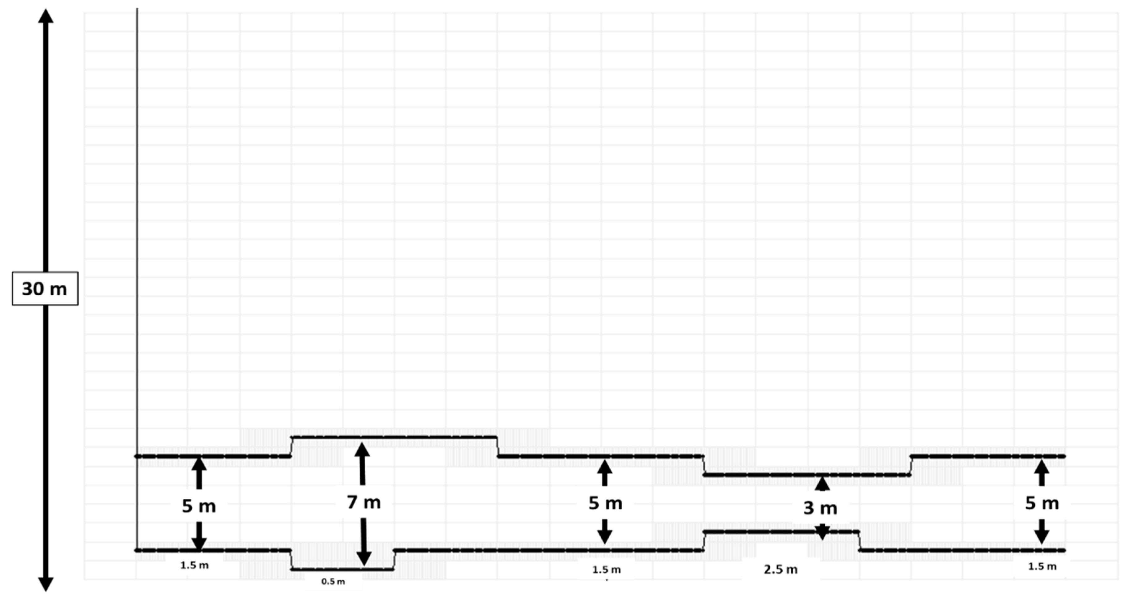
In this model, the producer and injector follow complex trajectories with variable lateral separating distances ranging from three meters at the narrowest point to seven meters at the widest point. The dual-string base case has two injection points and two production points (heel and toe). The optimized OCD’s case will have OCDs deployed along the injector long tubing, while the producer maintains its original dual-string completion system.
The dual-string completion scheme is shown in Figure 2, where 4 1/2″ short and long tubing strings are packed into a 9 5/8″ slotted liner.
3.2. Optimization Analysis with OCD Deployment
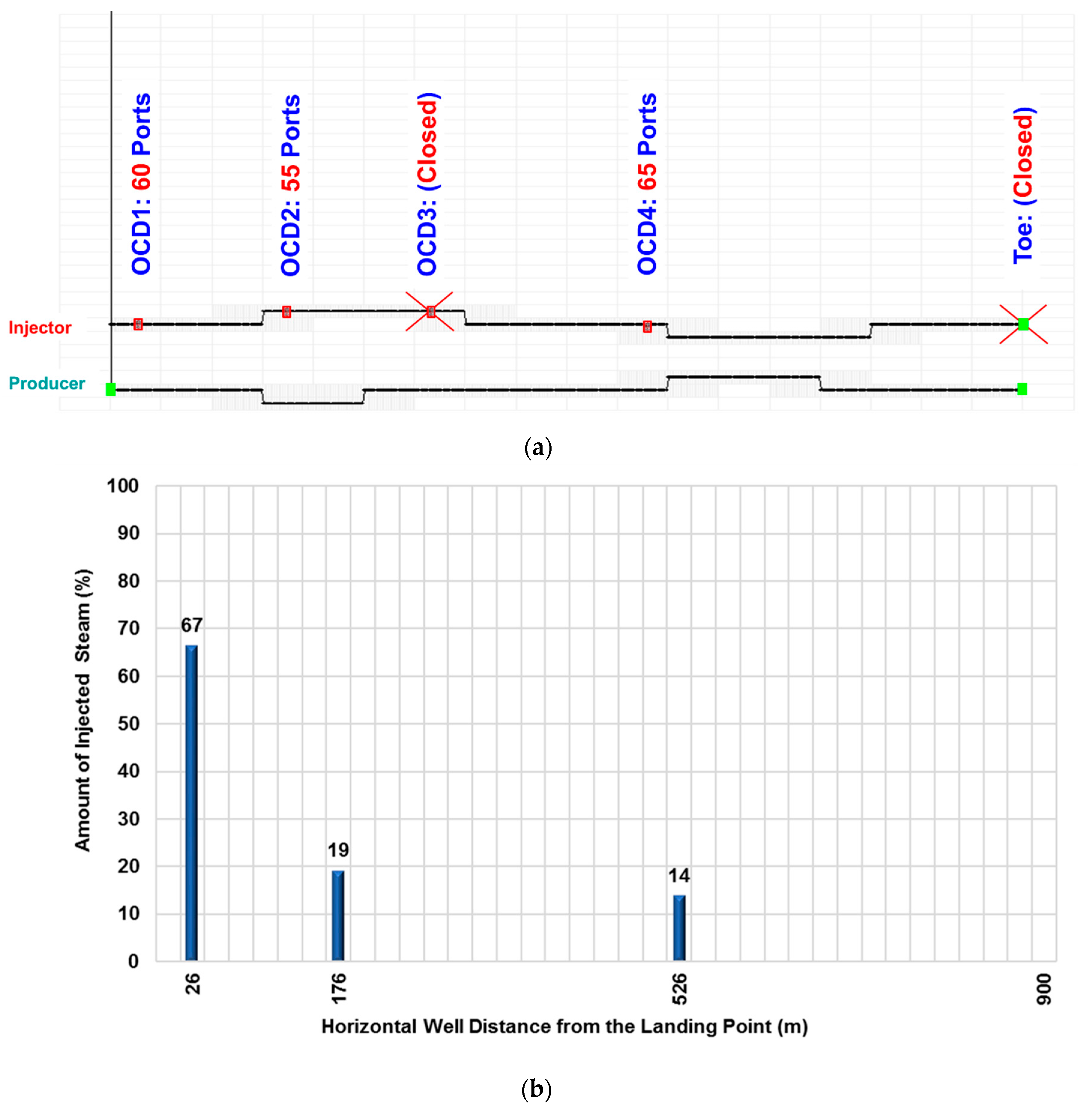
For the optimization work, four OCD’s were deployed along the long tubing of the injector at 26 m, 176 m, 326 m and 526 m away from the landing point (Figure 3). Another injection point is the fully open-to-flow toe. The producer maintained its original dual-string completion scheme.
3.2.1. Short-Term Optimization of Number of Ports
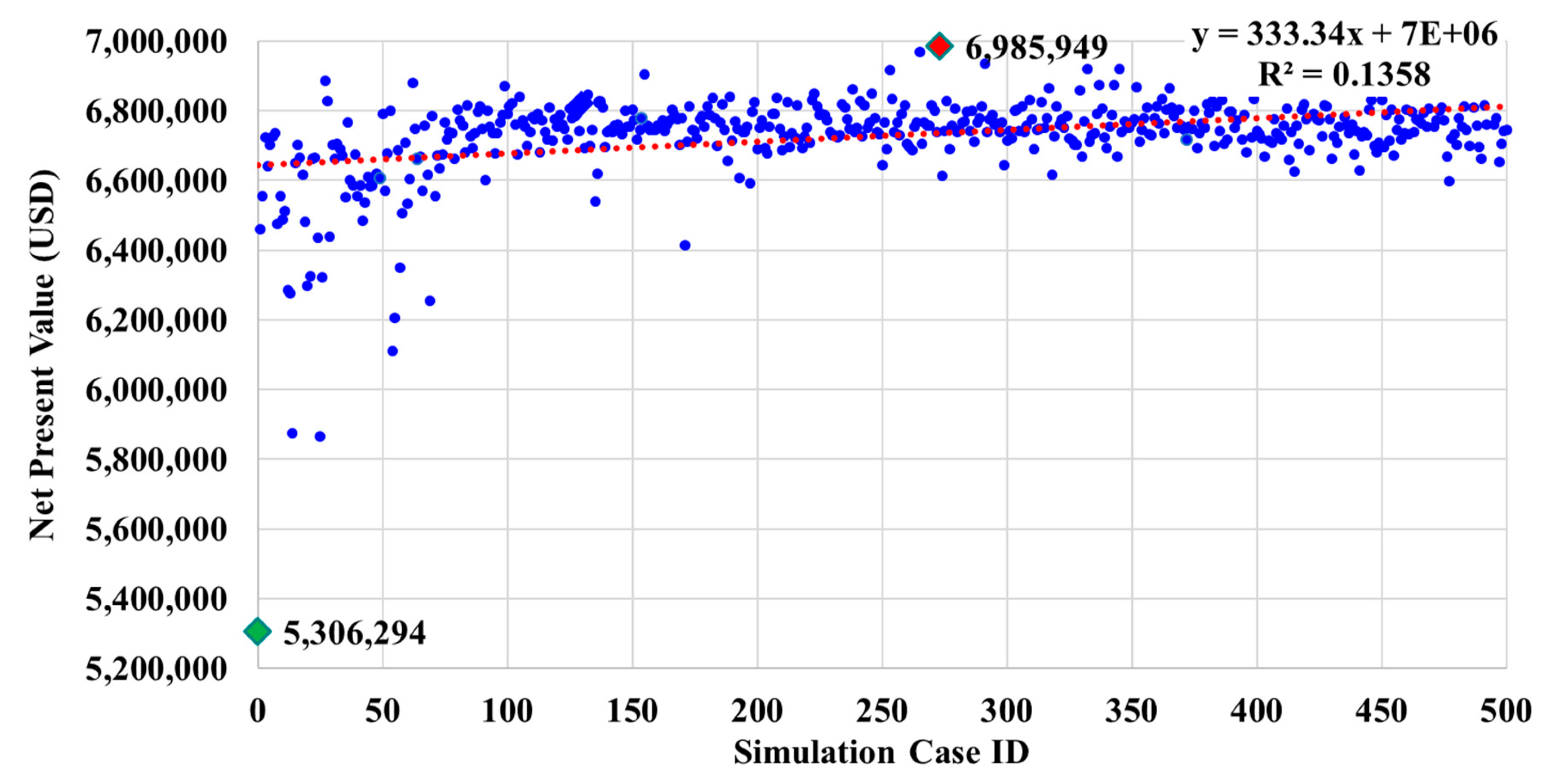
Short-term optimization results are shown in Figure 4. The conventional dual-string case has an NPV of $5,306,924, while the optimum case has a $6,985,949 NPV; that is, more than a 31% increment in NPV.
3.2.2. Long-Term Optimization of Number of Ports
The top 50 short-term cases were simulated for longer periods. Results reveal that the optimum case has a nil number of ports for OCD#3. Furthermore, the open toe does not contribute to flow. The remaining OCDs have 60, 55, and 65 ports for OCD#1, OCD#2, and OCD#4, respectively. As shown in Figure 5, the NPV of the optimum case is $21,730,098, and that is about 5% higher than the conventional dual-string well completion.
Simulation cases beyond the top 50 cases were run until the end of SAGD project life to confirm the decreasing trend of the NPV for long-term simulations according to the short-term NPV ranking. Results are shown in Figure 6. Negative general solutions trend line can be noticed indicating that increment of NPV is proportional to the case order.
Figure 7 shows the completion scheme of the wellbore trajectories with the OCD locations and number of ports.
3.2.3. Optimum Number of Ports
Figure 8 presents the number of ports for the top five optimum cases. In this figure, yellow squares are number of ports for OCD#1 that range from 60–70, red diamonds OCD#2 range from 55–65, green triangles OCD#3 range from 0–20, and blue circles OCD#4 range from 50–65. Results show that the number of ports for each OCD is relatively close for these optimum solutions, which indicate that the algorithm has converged towards the global optimum.
3.3. Results Analysis
3.3.1. Steam Distribution Using OCDs
Figure 9 shows the contribution of each single OCD to the total amount of steam injected at the end of the SAGD stage. A total of 65% of the steam has been injected at the heel section of the well (via OCD#1), 19% via OCD#2, and 14% via OCD#4.
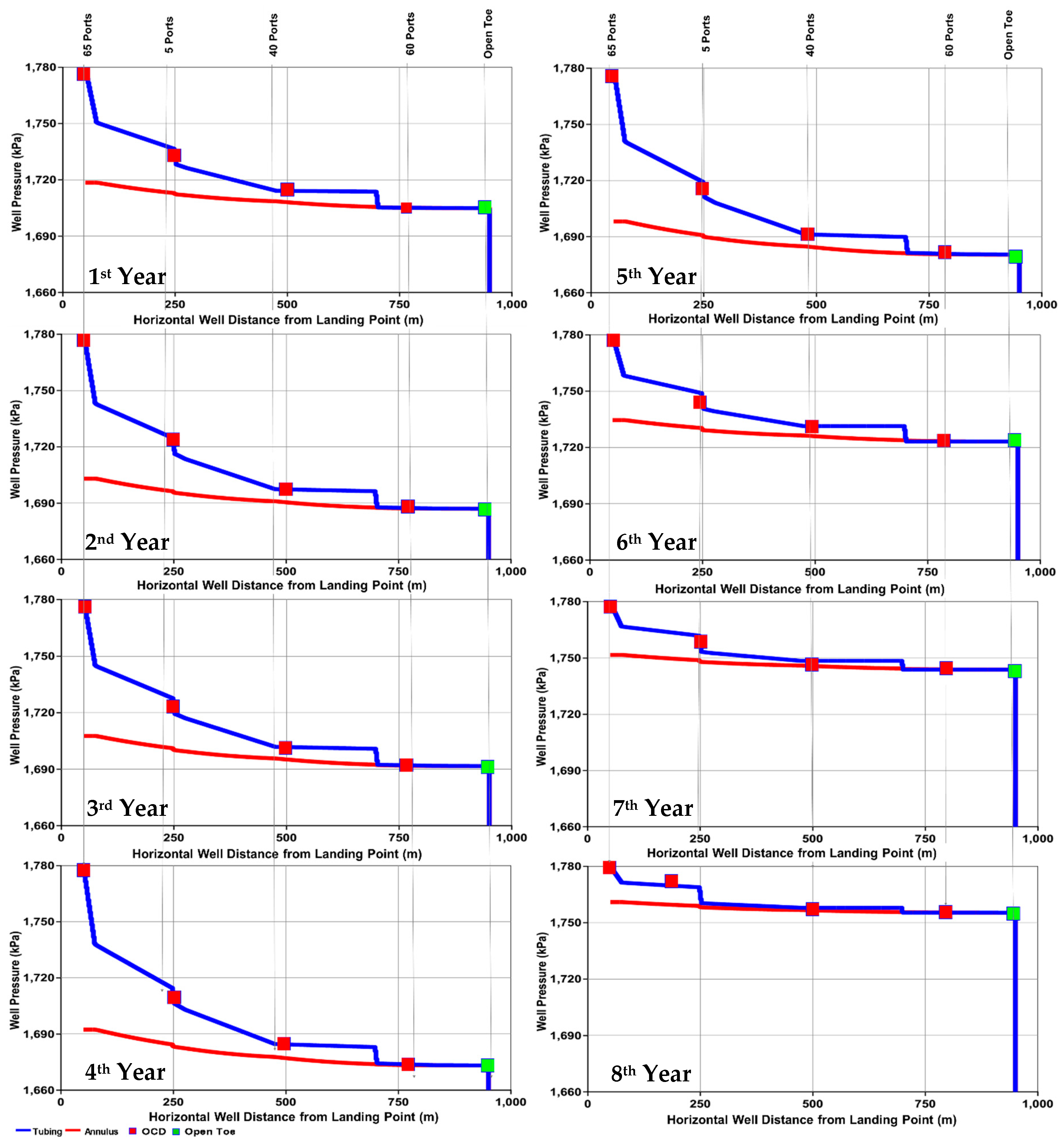
3.3.2. Injector Tubing/Annulus Pressure Profiles
Figure 10 shows tubing/annulus pressure profiles for the optimum OCD case. The largest amount of steam has been injected via OCD#1. The reduction in pressure drop at later SAGD stages reduced the contribution of OCD#2 and OCD#4 over time.
3.3.3. Comparison with Dual-String Case
• Pressure Profiles
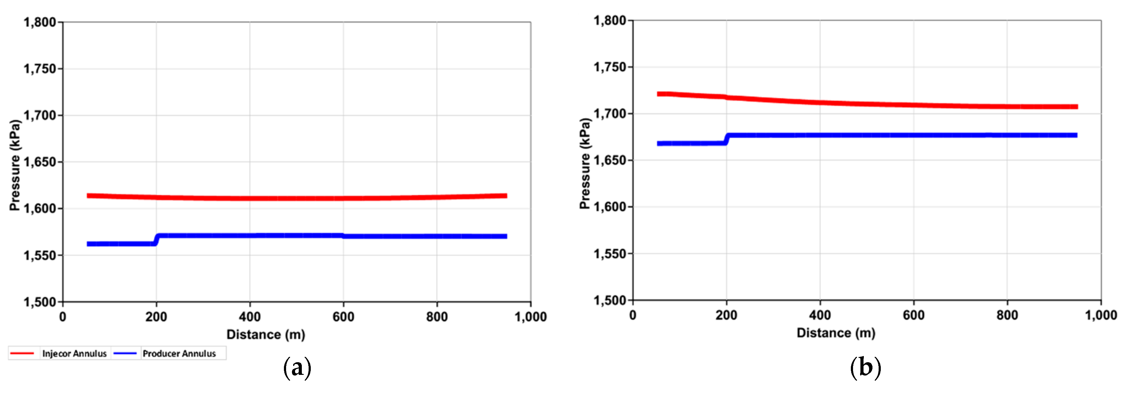
Figure 11 shows pressure profiles of the optimized OCD and dual-string cases inside the injector long tubing at the end of the third year. Results indicate 175 kPa frictional pressure losses from the heel to toe of the injector for the dual-string case, while it is only about 85 kPa for the optimized OCD model. Also, pressure profiles inside the long injector for both cases are affected by the wellbore trajectory excursions. The outcome, as shown in Figure 12, is higher annular pressures for the optimized OCD’s case (Figure 12b) resulting in an enhancement in the overall SAGD operating conditions compared to dual string case (Figure 12a).
• Steam Chamber Growth
Figure 13 depicts temperature maps for the optimized OCD and dual-string cases for three years. A more uniform and consistent steam chamber growth can be noticed for the optimized OCD case. Furthermore, it can be observed that the injected steam at the toe section of the dual-string case has no efficient heating effect during the first 1.5 years, and that is consistent with the optimized OCD’s case where the toe section does not contribute to the steam injection.
• Steam Distribution
Figure 14 shows steam injection distributions for three different cases at the end of the first year of SAGD. In the first case (Figure 14a), 100% of the injected steam is delivered at the toe. The distribution of injected steam and the temperature map in the reservoir indicates little steam penetration at the heel and toe segments, hence, a low SAGD performance. However, steam chamber will preferentially develop in the regions with minimum vertical separation distance between the horizontal sections.
The second case is with dual-string completion scheme (Figure 14b), which shows a better steam distribution along the well and a more enhanced steam chamber compared to the previous case. However, results still indicate little steam penetration at the toe segment.
In the third case (Figure 14c), where OCD’s have been deployed, results indicate 66% steam delivery through OCD#1 at the heel, 19% through OCD#2, and 12% through OCD#4. The outcome is a more even steam chamber growth and steam delivery into the formation. The segment with 7-m separation still demonstrates a poor performance compared to other segments. However, this segment will be swept by steam as SAGD continues beyond the first year. Figure 14d–f represents the cumulative steam injected into the formation through the annulus for the three cases (single tubing, dual-string and OCD cases), whereas Figure 14g–i represents the cumulative steam injected into the annulus through the long tubing or the OCDs for the three cases.
• Production Data
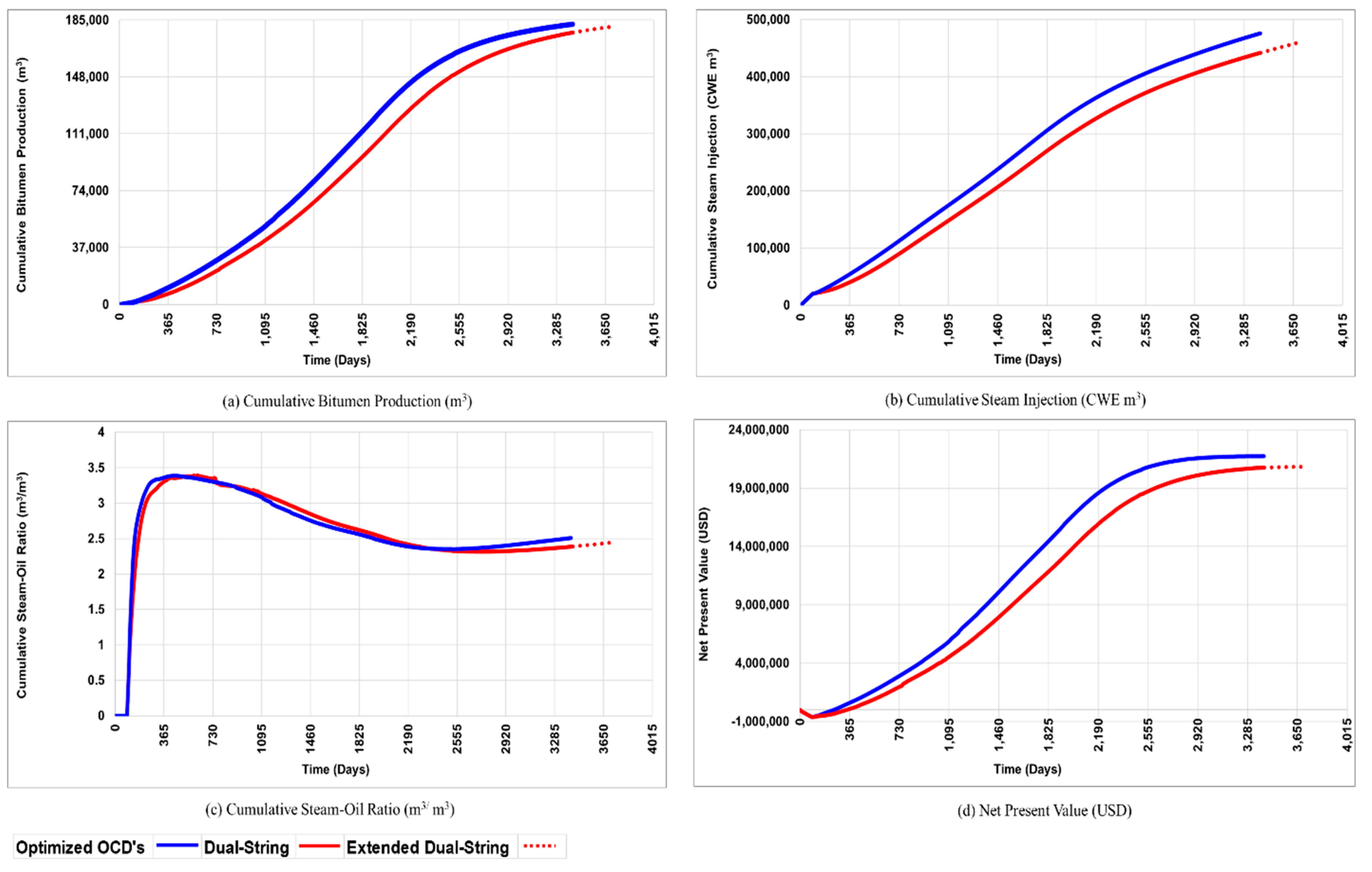
Figure 15 compares the performances of the models with the optimized OCD and dual tubing. For both cases, SAGD simulation runs have been terminated after the daily NPV increment becomes zero (ΔNPV/Δt = 0). The dual-string case was terminated after 3628 days (9.9 years) of SAGD operation, while the optimized OCD’s case was terminated after 3316 days (nearly 9.1 years). The optimized OCD case shows a 4% enhancement in NPV compared to the corresponding dual-string case; that is, equivalent to more than $900,000 positive cash flow. A comparison of SAGD performance data of both cases at the same termination time (9.1 years) indicates a better NPV enhancement for the optimized case by as much as 5%.
4. Discussion
Temperature maps in dual-string completion case show a poor steam chamber growth and a higher liquid level at the toe and 7-m vertical separating sections. Furthermore, steam does not stay at a high separating distance and toe sections due to gravity.
Optimization results show 60 ports for OCD#1, 55 ports for OCD#2, zero ports for OCD#3 and 65 ports for OCD#4, in addition to a nil contribution from the open toe. 67% of the total amount of steam is injected at the heel section (OCD#1), and the remaining 33% is distributed at different sections along the well pair via OCD#2 and OCD#4 only. The vast majority of steam injected via tubing (67%) enters the injector annulus via OCD#1 and then travels to other sections of the injector through the large annular space. The remaining amount of steam (25%) is injected at different sections of the injector OCD#2 and OCD#4. Additionally, the optimization work has shown that there is no need to inject steam via OCD#3 and toe sections.
It is observed that in the optimal number of ports in this specific case study with wellbore undulations, OCD#1 is the major contributor to the total amount of steam injected. This is due to the large annular cross-sectional area between the slotted liner and the tubing compared to the tubing diameter. The slotted liner has 9 5/8″ diameter (72.6 in2 cross-sectional area), and the tubing has 4 1/2″ diameter (15.9 in2 cross-sectional area), and that means the annular space between the slotted liner and the tubing is more than 3.5 times larger in cross-sectional area (56.9 in2) compared to the same for the tubing. The injected steam tends to take the path that has the least resistance to flow.
In real-life applications, SAGD well pairs are not perfectly horizontal; and wellbore undulations reduce production performance. Similarly, heterogeneities in reservoir rock properties between the horizontal well pairs, together with permeability variations in the reservoir and flow baffles, impact steam chamber development. In this study, which includes undesired deviations in well pair trajectories, results show that optimal placement and design of flow control devices significantly improves production performance compared to conventional dual string configuration.
5. Conclusions and Recommendations for Future Work
Improvements of SAGD performance in the optimized OCD cases are mainly achieved by increasing overall amounts of injected steam, and delivering steam to areas that have poor sweep efficiencies and elevated SAGD operating conditions (producer and injector annulus pressure) due to minimized pressure losses to friction. For those reasons, all optimized OCD’s cases have slightly higher cumulative injected steam and terminal cSOR (compared to their corresponding dual-string injection cases). However, they are still considered as optimum cases because they have higher cumulative oil production and NPV.
The optimum number of ports in each OCD for the optimized case mainly depends on the available pressure drop across the OCD between the injector tubing and annuls, in addition to the vertical separating distance between the horizontal well pairs and other reservoir and wellbore parameters. The scope of this paper was limited to the improvement of the SAGD process’s performance by optimization of design and placement of OCD’s along the injector. However, the involvement of IC’s on the producers, simultaneously with OCDs may yield more improvements in SAGD operations.
Performance of other SAGD reservoirs with different geological settings can also be enhanced by properly-optimized placement of OCDs/ICDs. Some of the different reservoir types that have not been covered in this research include SAGD reservoirs with bottom water, gas cap, low reservoir ceiling, mud channels, heterogeneous geological properties or a combination of all or some of those different settings. Besides, single well pair models do not capture the effect of steam chamber interactions. Steam chamber development along accretion packages of point bar deposits play an important role in the interaction between multiple well pairs and need further investigation. However, reservoir simulation run time and costs limit studies on the well pad scale that include geological details.
Author Contributions
Conceptualization, A.S., S.N., and A.N.; methodology, A.S.; software, A.S.; validation, A.S.; formal analysis, A.S.; investigation, A.S.; resources, A.S. and A.N.; data curation, A.S.; writing—original draft preparation, A.S., S.N., and A.N.; writing—review and editing, S.N.; visualization, A.S.; supervision A.N.; project administration, A.S. and A.N.; funding acquisition, A.N.
Funding
This research was jointly funded by Natural Sciences and Engineering Research Council of Canada (NSERC) and RGL Reservoir Management Inc., through a Collaborative Research and Development (CRD) funding program.
Acknowledgments
The authors would like to acknowledge Computer Modeling Group (CMG) company and its technical team for securing necessary software packages and their support.
Conflicts of Interest
The authors declare no conflict of interest.
Symbols
| Rt | Revenue, ($) |
| Et | Operation expenses, ($) |
| D | Annual discount factor |
| Tp | Project life time, years |
| tp | Project time step, years |
| Qo | Oil production rate, (STB⁄D) |
| Qw | Steam injection rate, (bbl of CWE⁄D) |
| ro | Oil price, ($⁄STB) |
| rw | Steam cost, ($/CWE bbl) |
| tk | Simulation time step |
| tref | Reference time, days |
| P | Pressure |
| T | Temperature |
Abbreviations
| 3D | Three-Dimensional |
| CMG | Computer Modeling Group |
| cSOR | Cumulative Steam-Oil Ratio |
| CWE | Cold Water Equivalent |
| DECE | Designed Exploration & Controlled Evolution |
| FCDs | Flow Control Devices |
| ICDs | Inflow Control Device |
| IHS | Inclined Heterolithic Stratification |
| LGR | Local Grid Refinement |
| LHS | Latin Hypercube Sampling |
| OCDs | Outflow Control Devices |
| SAGD | Steam-Assisted Gravity Drainage |
References
- Butler, R.M. Thermal Recovery of Oil and Bitumen; Prentice Hall: Englewood Cliffs, NJ, USA, 1991; pp. 1–528. [Google Scholar]
- Stalder, J. Test of SAGD Flow-Distribution-Control Liner System in the Surmont Field, Alberta, Canada. J. Can. Pet. Technol. 2013, 52, 95–100. [Google Scholar] [CrossRef]
- Stone, T.W.; Bailey, W.J. Optimization of Subcool in SAGD Bitumen Processes. In Proceedings of the 2014 World Heavy Oil Congress, New Orleans, LA, USA, 5–7 March 2014. Paper No. WHOC14-271. [Google Scholar]
- Medina, M. Design and Field Evaluation of Tubing-Deployed Passive Outflow-Control Devices in Steam-Assisted-Gravity-Drainage Injection Wells. Soc. Pet. Eng. 2015, 30, 283–292. [Google Scholar] [CrossRef]
- Nejadi, S.; Hubbard, S.M.; Shor, R.J.; Gates, I.D.; Wang, J. Optimization of Placement of Flow Control Devices under Geological Uncertainty in Steam Assisted Gravity Drainage. In Proceedings of the SPE Thermal Well Integrity and Design Symposium, Banff, AB, Canada, 27–29 November 2018; Society of Petroleum Engineers: Richardson, TX, USA, 2018. [Google Scholar]
- Kyanpour, M.; Chen, Z. Design and Optimization of Orifice based Flow Control Devices in Steam Assisted Gravity Drainage: A Case Study. In Proceedings of the SPE Heavy and Extra Heavy Oil Conference, Medellín, Colombia, 24–26 September 2014; Society of Petroleum Engineers: Richardson, TX, USA, 2014. [Google Scholar]
- Noroozi, M.; Melo, M.; Montoya, J.; Neil, B. Optimizing Flow Control Devices in SAGD Operations: How Different Methodologies are Functional. In Proceedings of the SPE Thermal Well Integrity and Design Symposium, Banff, AB, Canada, 23–25 November 2015; Society of Petroleum Engineers: Richardson, TX, USA, 2015. [Google Scholar]
- Banerjee, S.; Hascakir, B. Design of flow control devices in steam-assisted gravity drainage (SAGD) completion. J. Pet. Explor. Prod. Technol. 2018, 8, 785–797. [Google Scholar] [CrossRef]
- Riel, A.; Burton, R.C.; Vachon, G.P.; Wheeler, T.J.; Heidari, M. An Innovative Modeling Approach to Unveil Flow Control Devices Potential in SAGD Application. In Proceedings of the SPE Heavy Oil Conference, Calgary, AB, Canada, 10–12 June 2014; Society of Petroleum Engineers: Richardson, TX, USA, 2014. [Google Scholar]
- Suncor Energy. Suncor MacKay River Project 2014 AER Performance Presentation: Subsurface Commercial Scheme Approval No. 8668. AER. Available online: https://www.google.com.hk/url?sa=t&rct=j&q=&esrc=s&source=web&cd=1&ved=2ahUKEwjs74DUwpXkAhXDy4sBHfyDBS0QFjAAegQIBhAC&url=https%3A%2F%2Fwww.aer.ca%2Fdocuments%2Foilsands%2Finsitu-presentations%2F2014AthabascaSuncorMacKaySAGD8668.pdf&usg=AOvVaw0bDFH_wPpnTN_Clw5XI1Yo (accessed on 8 July 2019).
- Ghesmat, K.; Zhao, L. SAGD Well-Pair Completion Optimization Using Scab Liner and Steam Splitters. J. Can. Pet. Technol. 2015, 54, 387–393. [Google Scholar] [CrossRef]
- Sidahmed, A.; Nouri, A.; Kyanpour, M.; Nejadi, S.; Fermaniuk, B. Optimization of Outflow Control Devices Placement and Design in SAGD Wells with Trajectory Excursions. In Proceedings of the SPE International Heavy Oil Conference and Exhibition, Kuwait City, Kuwait, 10–12 December 2018; Society of Petroleum Engineers: Richardson, TX, USA, 2018. [Google Scholar]
- Sidahmed, A. Optimization of Outflow Control Devices Design in Steam-Assisted Gravity Drainage Models with Wellbore Trajectory Excursions. Master’s Thesis, University of Alberta, Edmonton, AB, Canada, November 2018. [Google Scholar]
- Becerra, O.; Kearl, B.; Sanwoolu, A. A Systematic Approach for Inflow Control Devices Testing in Mackay River SAGD Wells. In Proceedings of the SPE Heavy Oil Conference, Calgary, AB, Canada, 10–12 June 2014; Society of Petroleum Engineers: Richardson, TX, USA, 2014. [Google Scholar]
- Jones, C.; Morgan, Q.; Beare, S.; Awid, A.; Parry, K.; Design, T. Qualification and Application of Orifice Type Inflow Control Devices. In Proceedings of the International Petroleum Technology Conference, Doha, Qatar, 7–9 December 2009; Society of Petroleum Engineers: Richardson, TX, USA, 2009. [Google Scholar]
- McKay, M.D.; Beckman, R.J.; Conover, W.J. A comparison of three methods for selecting values of input variables in the analysis of output from a computer code. Technometrics 2000, 42, 55–61. [Google Scholar] [CrossRef]
Figure 1.
Outflow control devices’ (OCDs’) number of ports optimization process workflow.

Figure 2.
Well completion scheme for the base case.

Figure 3.
Well completion scheme for tubing-deployed OCDs.

Figure 4.
OCD’s optimization results (short-term).

Figure 5.
Long-term optimization results.

Figure 6.
Long-term net present value (NPV) calculations.

Figure 7.
Optimum OCD cases.

Figure 8.
Optimum number of ports for top five designs.

Figure 9.
Distribution of injected steam among OCDs at the end of the SAGD’s project life. (a) SAGD well pair; (b) cold water equivalent (CWE) of cumulative steam injected through injector OCDs at the end of SAGD (CWE m3).
Figure 9.
Distribution of injected steam among OCDs at the end of the SAGD’s project life. (a) SAGD well pair; (b) cold water equivalent (CWE) of cumulative steam injected through injector OCDs at the end of SAGD (CWE m3).

Figure 10.
Optimum OCD’s case injector tubing/annulus pressure profiles.

Figure 11.
Injector long tubing pressure profiles, optimized OCDs (blue line), and dual-string cases (red line).
Figure 11.
Injector long tubing pressure profiles, optimized OCDs (blue line), and dual-string cases (red line).

Figure 12.
Annular pressure profiles. (a) Dual-string case; (b) optimized OCD case.

Figure 13.
Steam chamber growth of the optimized OCD and dual-string cases.

Figure 14.
Distribution of injected steam at different points after one year of SAGD. (a) Temperature map (single tubing); (b) temperature map (dual-string); (c) temperature map (OCDs); (d) cumulative steam injected into the formation through the annulus (single tubing); (e) cumulative steam injected into the formation through the annulus (dual-string); (f) cumulative steam injected into the formation through the annulus OCDs (OCDs); (g) cumulative steam injected into the formation through long tubing (single tubing); (h) cumulative steam injected into the formation through long and short tubing (dual-string); (i) cumulative steam injected into the formation through long tubing OCDs (OCDs).

Figure 15.
SAGD performance data of optimized OCDs and dual-string cases.


Table 1.
Fixed parameters in the optimization process.
| Item | Value |
|---|---|
| SAGD Process Termination Criteria | ΔNPV/Δt = 0 |
| OCD’s Port Size (mm) | 10 |
| Number of OCDs per Well (Max.) | 4 |
| Number of Ports per OCD (Min.) | 0 |
| Number of Ports per OCD (Max.) | 70 |
| Number of Ports Increment | 5 |
Table 2.
OCD’s optimization steps.
| Step -1 | Step -2 |
|---|---|
| Short-Term Optimization | Long-Term Optimization |
| Duration: 3 Years | Duration: (SAGD project life, i.e.,: ΔNPV/Δt = 0) |
| Number of OCD’s: 4 | Number of OCD’s: 4 |
| OCD’s Port Size: 10 mm | OCD’s Port Size: 10 mm |
| Injector Completion: Tubing-Deployed OCD’s (Long Tubing + OCD’s) | Injector Completion: Tubing-Deployed OCD’s (Long Tubing + OCD’s) |
| Producer Completion: Dual-String (Long Tubing + Short Tubing) | Producer Completion: Dual-String (Long Tubing + Short Tubing) |
Table 3.
Steam assisted gravity drainage (SAGD) 3D model reservoir properties.
| Property | Unit | Value |
|---|---|---|
| Depth | m | 110 |
| Initial Reservoir Pressure | kPa | 400 |
| Initial Reservoir Temperature | °C | 7 |
| Horizontal Permeability | md | 1500 |
| Vertical Permeability | md | 825 |
| Average Porosity | % | 32 |
| Net-to-Gross Ratio | % | 95 |
| Average Oil Saturation | % | 85 |
© 2019 by the authors. Licensee MDPI, Basel, Switzerland. This article is an open access article distributed under the terms and conditions of the Creative Commons Attribution (CC BY) license (http://creativecommons.org/licenses/by/4.0/).
Share and Cite
MDPI and ACS Style
Sidahmed, A.; Nejadi, S.; Nouri, A. A Workflow for Optimization of Flow Control Devices in SAGD. Energies 2019, 12, 3237. https://doi.org/10.3390/en12173237
AMA Style
Sidahmed A, Nejadi S, Nouri A. A Workflow for Optimization of Flow Control Devices in SAGD. Energies. 2019; 12(17):3237. https://doi.org/10.3390/en12173237
Chicago/Turabian StyleSidahmed, Anas, Siavash Nejadi, and Alireza Nouri. 2019. "A Workflow for Optimization of Flow Control Devices in SAGD" Energies 12, no. 17: 3237. https://doi.org/10.3390/en12173237
Note that from the first issue of 2016, this journal uses article numbers instead of page numbers. See further details here.