Hot Metal Temperature Prediction at Basic-Lined Oxygen Furnace (BOF) Converter Using IR Thermometry and Forecasting Techniques


Polytechnic School of Engineering, University of Oviedo, 33204 Gijón, Spain
*
Author to whom correspondence should be addressed.
Energies 2019, 12(17), 3235; https://doi.org/10.3390/en12173235
Submission received: 18 June 2019
/
Revised: 20 July 2019
/
Accepted: 14 August 2019
/
Published: 22 August 2019
Abstract
:In oxygen steelmaking, the charge calculation strongly depends on hot metal temperature prediction. Although a hot metal temperature drop from the blast furnace in a steel plant may be too complex to be accurately modeled in detail, the combined use of sensors and statistical models can improve temperature estimation and result in better cost, quality and productivity, as well as lower emissions. In order to develop a simple but robust method for hot metal temperature forecasting, the suitability of infrared thermometry and time series forecasting has been studied. Simultaneous infrared thermometer measurement and video recording was used for designing the processing of the thermometer signal. The resulting temperature estimations are in good agreement with disposable thermocouple measurements giving an error of 11 °C with 60% reliability (chances of obtaining a successful output). Conversely, the time series approach was based mainly on the AutoRegressive Integrated Moving Average (ARIMA) model in which five additional process variables were introduced as exogenous predictors, as well as using a moving window of past observations for continuous model training. The resulting error was 15 °C with more than 90% reliability. Combining measuring and modeling approaches reduced the error to 13 °C with 100% reliability, thereby providing a hybrid procedure that has long-term stability and is self-adaptive to varying production scenarios.
1. Introduction
Despite its 70 years of history, oxygen steelmaking still faces continuous challenges regarding productivity, quality, cost and environment. Consequently, a combination of breakthrough process innovations, along with incremental improvements in sensors and control models, have been addressed in recent years.
Oxygen steelmaking process begins at the blast furnace (BF), where iron ore is reduced into a carbon-rich molten iron called hot metal. A second stage takes place in a basic-lined oxygen furnace (BOF), wherein the hot metal is mixed with steel scrap and transformed into liquid steel by blowing in oxygen and making use of inert gases and other additives. It is a batch process where around 200 t of hot metal are used to produce 300 t of liquid steel, approximately. Each batch is often called “a heat”; therefore, this term will be used hereinafter. Oxidation of hot metal impurities such as C, Si or P inside the BOF provides enough energy for heating up and melting the scrap and raising the temperature of the melt from initial conditions of around 1200 °C up to a final temperature target above 1600 °C. A joint overview of BF and BOF processes is provided by Ghosh [1], while a detailed analysis of the BOF process can be found in Miller [2].
Hot metal is usually transported by railway from the BF to the BOF using a special lined vessel, called torpedo car or, succinctly, torpedo. At the BOF shop, the process computer runs a charge model in order to calculate the amounts of hot metal and scrap that must be loaded into the BOF to produce the required target steel in terms of mass, composition and temperature. For a given target steel, the hot metal to scrap ratio mainly depends on hot metal temperature and composition. However, by using suitable exo- or endothermic additives, a wide range of hot metal ratios can satisfy both mass and energy balances. Hence, an optimum hot metal ratio, regarding cost, quality, productivity or emissions, can be found by the charge model. Since the raw materials account for a significant part of steel cost, the performance of the charge model, which in turn depends on the accuracy of hot metal temperature prediction, is essential for the steelmaker.
While hot metal composition remains rather stable from BF to BOF, its temperature undergoes a variable drop, so its exact value is not known at charge model runtime, only being measured later, just before loading the BOF. This uncertainty could be only partially overcome by direct measurement of the hot metal temperature in advance. Nevertheless, this approach presents certain practical disadvantages and therefore, a more or less rough estimation is used instead.
Hot metal operations inside an integrated steel mill can be quite complex since they may comprise several BFs, BOFs together with associated pretreatment facilities as well as numerous transport vessels as torpedoes and ladles. However, the main sub-processes concerning the scope of this research are outlined in Figure 1. Management of the BF-BOF connection is key for steelmaking costs on account of its impact on raw materials, energy and emissions. Therefore, its optimization has received much attention and has been usually approached from a holistic perspective [3,4]. On the contrary, existing research on hot metal temperature tends to focus on the individual sub-processes, aimed at understanding or predicting its behavior.
From a BF perspective, temperature of tapped hot metal is predicted and monitored as a mean to describe the thermal conditions inside the hearth of the furnace. Temperature is controlled with the aid of advanced mathematical models in an attempt to achieve an approximate knowledge of its complex behavior [5,6]. Usually, the actual hot metal temperature is intermittently measured by an operator using disposable thermocouples. Since this method only provides partial information, continuous determination of temperature by means of combined modeling and indirect measurements is a growing area of interest in BF [7,8,9,10], but comparable efforts for BOF have not yet been reported [11,12].
Heat transfer in torpedo car has attracted the attention of researchers due to its effects on the thermomechanical behavior of the refractory lining and on molten iron metallurgy [13,14,15]. There are also some studies on the optimum scheduling of torpedo cycling, in which thermal losses are identified as an important part of the cost structure, being a function of the elapsed time between pick up and drop of the hot metal [16] and also the empty time [17]. Concerning the effect of heat transfer on hot metal temperature at BOF shop, both theoretical [18] and experimental [19] research has been carried out, but a complete model, such as those for steel ladles [20], has not yet been published.
Thus, the evolution of hot metal temperature from BF to BOF appears to be highly complex for modeling accurately in real time, since it is an intermittent process in which each BF iron batch is divided among torpedoes and then remixed at the BOF shop with additional hot metal that could have come from a different BF and have undergone a totally different process. Moreover, regarding hot metal temperature drop, there are many relevant phenomena that are difficult to properly measure or even characterize. For instance, heat lost in the soaking out of the lining during filling is a function of the thermal state of the lining prior to filling, which depends mainly on its thickness and past thermal history. Provided that the lining thickness is known, the thermal state could be calculated for a completely cold or for a totally soaked torpedo car, but the same would be very hard for intermediate cases, especially bearing in mind that a significant amount of heat is lost in re-melting solid iron and slag remnants inside the vessel [19]. Moreover, it is also difficult to characterize the heat losses in open streams during hot metal pouring and only approximate estimations can be formulated, on account of their variable shape and velocity [18].
Although the temperature evolution of hot metal between BF and BOF is always important, it is crucial in sites of complex layout with several BFs feeding distinct and distant BOF shops and many operating torpedo cars and ladles [19,21,22,23]. In these cases, prediction and control of temperature during hot metal transportation becomes critical, but it may be also more difficult to address, since the scarcity of important data, or missing or wrong data, and greater uncertainties are more likely to occur.
The aim of this research is to obtain a simple procedure for hot metal temperature forecasting at the BOF shop from available existing plant data. This temperature estimation will be used as an input for the charge model; since an accurate prediction is not feasible, an enhanced estimation would at least reduce the charge model error and result in environmental, productivity and cost improvements [24,25,26].
In this study, the feasibility of infrared thermometry as an early estimator of actual hot metal temperature at BOF shop is investigated and its accuracy and reliability are assessed. Moreover, after selecting suitable predictor variables, the modeling approach is presented by comparing several alternatives of increasing complexity and accuracy. Finally, since the different measuring and modeling approaches are found to be complementary, a combined methodology of indirect measurement and statistical forecasting is proposed for providing the best available hot metal temperature prediction to be used by the charge model.
2. Materials and Methods
As already mentioned, the hot metal temperature must be estimated before calculating how much hot metal is required for the BOF process. The better this prediction, the more accurate the BOF charge model calculation. At first glance, four main approaches could be envisaged to improve temperature determination: direct measurement, indirect measurement, mechanistic modeling, and data-driven modeling. Direct measurement using dip thermocouples before completing hot metal preparation at the BOF shop will incur in time and productivity losses. By contrast, an early indirect measurement during hot metal transfer could provide a reliable temperature assessment in advance.
2.1. Infrared Thermometry
From an accuracy point of view, a direct measurement with disposable dip thermocouples [27] seems to be the best option. However, this measurement can only be performed when the torpedo is very close to the transfer point. This implies that hot metal charge calculation should wait until the last minute, delaying the scrap preparation and the whole BOF process, resulting in important productivity losses. Moreover, if the existing measurement equipment were to be used, it may be necessary to pour a minimum quantity of hot metal into the ladle, then move it to the measurement position, and finally, move it back to the transfer position to complete the hot metal transfer while simultaneously completing the scrap preparation. As a side effect, the resulting temperature would not be as accurate as a straight measurement just before loading the converter. Conversely, indirect measurement using infrared (IR) thermometry at the beginning of hot metal pouring from torpedo to ladle (TIR in Figure 1) would allow an early temperature estimation avoiding interferences, and hence, productivity losses.
In order to assess the feasibility of IR thermometry for contactless estimation of the hot metal temperature, a LAND-MZ IR thermometer with 0.55 μm wavelength, 1200 to 1700 °C temperature range and manual focus from 0.5 m to infinity was used. The IR device was placed aimed at the hot metal stream from a distance of about 11 m, covering different orientations and two hot metal transfer positions, as depicted in Figure 2. Emissivity compensation was adjusted to 0.4 and focal length was fixed to infinity, which corresponded to a field of view (FOV) of 200:1, providing a measurement spot with less than 100 mm in diameter on the hot metal stream surface. An output signal of 4–20 mA was sampled at 5 sps, A/D converted and stored. The acquisition started with the first reading above 1201 °C and ended after 150 consecutive samples below 1201 °C. A digital video camera was mounted in the thermometer viewfinder, recording the hot metal stream at 30 fps. The obtained frames were compared with instantaneous IR temperature readings.
The following complementary data were acquired from process databases for correlating the indirect measurements with actual temperatures: initial and final time of each partial pouring, partial mass transferred from each torpedo, total hot metal mass loaded into the ladle, and actual hot metal temperature and time of measurement in the ladle.
2.2. Time Series Forecasting
A fundamental detailed model attempting to describe the underlying phenomena appears to be unpractical here, since several of the required input variables and parameters would be more difficult to obtain than the variable to be modeled itself. However, statistical modeling should be capable of extracting improved knowledge and provide useful forecasts from readily available data. However, while data-driven models allow for obtaining predictions that can fit well with observations, this approach may present serious issues regarding generalization and long-term stability [28,29]. For this reason, a continuous updating process is applied to the model parameters in order to guarantee that prediction error is kept as low as possible in the following forecasts.
In this section, the most adequate predictor variables are selected before testing several simple forecasting methods. Later, more complex forecasting models are considered. The purpose of this approach is twofold: firstly, a simple model provides a useful benchmark for more sophisticated models; secondly, it can be used as a backup procedure by the plant process computer in absence of any of the data required by more complex models.
2.2.1. Variable Selection and Normalization
Among the different available variables in process databases, only six that were judged relevant and with no more than 10% missing data points were taken into account. They are represented in Figure 1 and described in this section.
The initial hot metal temperature T0, is obtained from discrete measurements performed in the iron runner at the exit of the tap hole during blast furnace tapping [30]. In general, three measurements are taken by cast: firstly, just after piercing the tap hole; secondly, when the slag starts to flow out; and finally, about the end of the cast. Hot metal temperature measurement obtained at the beginning of the tapping tends to be lower than the successive measurements, since the first hot metal comes from the lower part of the hearth, which is colder. As tapping time progresses, hot metal comes straight from the ore melting and it is hotter. The measured tapping temperature along with its timestamp is essential for BF process control, and therefore, it can be considered a robust variable. It must be kept in mind that neither the tapping rate nor the time when the tapping hole is open are regular. Moreover, the number and instant of temperature measurements taken in a cast may be irregular too. Temperature is assigned to the corresponding torpedo by time interpolation between consecutive measurements.
The elapsed time between temperature measurements in the BF and in the BOF ladle t, was taken as the effective transport time. Instead of taking three different time intervals, corresponding to torpedo car transport, pouring at BOF shop, and ladle holding, the total time was considered as a single input variable. Since hot metal pouring may extend over a significant time period, it was not always possible to clearly determine the limit between torpedo and ladle. Considering that heat losses in torpedo and ladle were found to be similar, as will be explained later, the proposed simplification worked well in practice.
At the pretreatment station, the total injection time of desulfurizing agent td, was taken as the representative variable for including the effect of this sub-process on thermal losses. Considering that mass flowrates of desulfurizing agent and inert gas are essentially constant, the main differentiating variable is the effective treatment time, which is a robust variable. Possible differences between agents were neglected, assuming that the main effect on temperature drop is caused by hot metal stirring.
The actual value of the predicted variable, the final hot metal temperature T, is measured in the ladle just before BOF loading. The hot metal in the ladle comes from two or more different torpedo cars, possibly from different BFs and having very different histories. The actual measured temperature T, is a robust variable, since it is required for running the second BOF process model (static model) and adjust the actual oxygen and the required endo- or exothermic additions [31]. The real values of this variable will be compared to the predicted ones, in order to evaluate the model performance.
The time while the torpedoes and ladle remained empty since the previous cycle tc, and tl, respectively, were chosen as a simplified but robust way of describing their initial thermal state. Other relevant aspects, such as actual lining thickness or the amounts of solidified slag and iron, could not be included because of poor data availability and inconsistencies. Moreover, the preheating of refractory lining was found to be not adequately measured since burners efficiency varied depending on several factors not fully described with the available data. Considering that the number of cases with previous preheating was less than 5%, those cases were left outside the scope of the model.
Due to the fact that hot metal in a ladle comes from two or more different torpedoes, the mass-weighted mean of the different torpedo-wise variables was taken into account for each ladle:
where x is the resulting variable value for the ladle, and mi and xi are the mass and the variable value for each torpedo, respectively.
In order to adjust the different dimensions and ranges of variables to an easily interpretable common scale and to avoid numerical instabilities, variables were pre-scaled to the interval [0,1]. It is well-known that widely different values and scales can cause instabilities that could affect the quality of the final model. Feature scaling was used to bring all values into the unit interval using the min–max normalization:
where X represents the original variable, x its standardized version, and min/max(X) are the observed limits of the historic register in the whole process database, as summarized in Table 1.
2.2.2. Simple Reference Methods
Very simple forecasting methods are often employed as a benchmark for other more complex models and can provide a fast prediction in the absence of detailed process data [32]. For example, it is a common practice to set a Standard Value (SV) for assuring, at least, a basic operating guidance in the event of model or process computer failure. For this case, temperature prediction is a constant standard value:
where cSV is usually the mean of historic observations, since it is expected to minimize the prediction error. The most cost-effective model is the Naïve Forecasting (NF), wherein the predicted value is equal to the last available observation, which may not be the immediately previous one:
where is the temperature forecast at current time index t and yt−w is the last observed temperature, and w is the lag index. Usually w = 1, but it can be greater when the immediate previous temperature could not be measured or stored.
Provided that the BOF process computer stores, at least, all of the previously measured temperatures, averaging the last w values should be a better approach. This method is known as Moving Average Smoothing (MAS):
2.2.3. Time Series Methods
Both stochastic and machine learning methods are often applied to time-series forecasting and, consequently, several studies have compared these two families of methods for specific case studies. A deep and extensive comparison between the two modeling cultures performed by Papacharalampous et al. [33] concluded that stochastic and machine learning methods may produce equally useful forecasts when applied to long-term studies. In this study, stochastic forecasting is applied to hot metal temperature prediction while machine learning based methods will be addressed in separated publications.
In a multiple regression model, the variable of interest is forecast using a linear combination of predictors. In an autoregressive model (AR), the variable of interest is forecast using a linear combination of past values of the variable while a moving average model (MA) uses past forecast errors in a regression-like model. An initial differencing step (I) is usually applied one or more times to eliminate the non-stationarities of the series. When differencing is combined with an autoregressive and a moving average model, a non-seasonal ARIMA model is obtained. ARIMA is an acronym for AutoRegressive Integrated Moving Average, where “integration” is the reverse of differencing [34]. ARIMA models aim to describe the autocorrelations in the data using the following general expression:
where c is a constant, ϕi are the regression coefficients for the autoregressive part, which is based in the p previous observations of the variable, and θi are the regression coefficients for the moving average part, which is based on the q past forecast errors. Hence, a generic model is noted as ARIMA (p, d, q), where p and q indicate the order of the AutoRegressive (AR) and Moving Average (MA) parts, respectively, and d is the order of the differencing step. In order to choose the optimum values for p, d and q, the Box-Jenkins method [35] is usually applied, as well as the Hyndman-Khandakar [34] algorithm.
It is important to note that, in the standard version of the ARIMA model shown in Equation (6) the coefficients c, ϕi and θi are kept constant for the successive forecasts, i.e., for every t. Here, by contrast, an improved approach is used instead, for ensuring model long-term performance in terms of stability and consistency:
where the (t,w) superscripts in the coefficients of Equation (7) indicate that for each new temperature forecast , the model is fitted again with the w previous observations of y; therefore, c, ϕi and θi are a function of yt−1, …, yt−w. The resulting model will be denoted as ARIMA (w, p, d, q), i.e., moving ARIMA based in the w previous observations.
When the five previously selected explanatory variables x1, … x5, (see Table 1) are introduced as eXogenous predictors in the ARIMA model, an ARIMAX model can be obtained [36]:
where βi are the regression coefficients for the explanatory variables xi.
However, in this research, the ARIMAX (w, p, d, q) model was fitted with the w previous observations, resulting in a moving ARIMAX model, i.e., ARIMAX (w, p, d, q):
3. Results
3.1. Infrared Thermometry
During a series of preliminary tests carried out on 30 hot metal ladles distributed over two weeks, IR temperature measurements together with video images where registered. The emissivity compensation was set at 0.4, as recommended by Mihalow [37] for this thermometer wavelength. Figure 3 shows a representative IR thermometer output obtained during the pouring of 150 t of hot metal from a torpedo into a ladle. It is a somewhat noisy curve in which, regardless of an important number of irregular drops and some peaks, several steady readings around 1370 °C can be identified. The 85th and 95th percentile of sampled temperatures are depicted with dashed lines at 1364 and 1369 °C.
Video recordings allowed us to identify the most common causes of signal fluctuation and perturbation and to understand under what circumstances the IR signal provided better information. As can be seen in Figure 4a, the stream was very thin during the initial 10 s of pouring and many sparks were produced resulting in no useful data. From t = 15 s to t = 30 s a much steadier reading was obtained, although some peaks and valleys can be observed in a short interval corresponding to the pouring of liquid slag (bright streaks in Figure 4b) and solid slag (dark spots in Figure 4c), respectively. Besides those perturbations, a reading around 1370 °C was obtained when the stream was almost clean as in Figure 4d. The narrow valley at t = 23 s corresponds to a hole produced in the stream, as can be seen in the frame sequence in Figure 4f–j. From t = 30 s onwards there is a much noisier signal due to the intermittent pouring of hot metal, caused by the final adjustment to weight set point. Under these circumstances the stream was often very narrow and contained many streaks of liquid slag, as seen in Figure 4e, when fumes were often produced.
From an initial set of 60 partial discharges of torpedoes, those with fewer useful samples were discarded resulting in 50 valid discharges, which correspond to 17 complete ladles. Sometimes the same torpedo was poured into two or three different ladles and the last discharge was not usually valid due to the very thin stream of hot metal. If this was the case, then the temperature was calculated from the previous discharge value and corrected for the temperature drop in the torpedo during the elapsed time with a coefficient CT (°C/min) that was taken as a parameter in temperature fitting. Total hot metal temperature was calculated as the mass-weighted mean of discharge temperatures on the ladle as indicated in Equation (1), with x = TIR, the effective hot metal infrared temperature for the ladle, and mi and xi = TIRi, the mass and the temperature for each of the N partial torpedo discharges, respectively. This temperature was corrected with a coefficient CL (°C/min), also taken as a parameter in temperature fitting, to account for the temperature drop in the ladle during the elapsed time from IR measurement to final temperature measurement with thermocouple.
Actual temperatures were measured in hot metal ladles using disposable type-K thermocouples. Linear regression was applied to fit TIR data to the actual temperature values together with parameters CT and CL. Results are shown in Table 2 and in Figure 5. Different statistical measures of IR temperature were assayed in order to filter the adverse effect of sparks, holes, solid slag spots and liquid slag streaks. The best fit was obtained when considering the 85–95th percentile of sampled temperatures for each partial discharge. The optimized values for CL and CT where found to be about 0.9–1.0 °C/min, which agreed very well with additional measurements performed in torpedo and ladle during the tests and also with the values reported by Du [21].
In order to assess the actual performance of a standalone IR thermometry industrial system, a second and more extensive trial was carried out in two different transfer positions over 168 heats. From this set, 63 measurements were not valid, mainly due to the fact that the FOV of the IR device not always matched stream location. Finally, 51 and 54 temperature predictions where obtained for transfer position 1 and transfer position 2, respectively. The settings for the IR sensor and signal processing were not modified with regard to the first trial: emissivity at 0.4, focus to infinity, sampling rate at 5 sps, percentile 95 as summary statistics, and CL = 0.9 °C/min. Since only heats with a complete discharge dataset were taken into account for this trial, a correction for torpedo holding time was not necessary.
Results of the second trial are summarized in Figure 6, where a good correspondence between IR and actual temperatures is observed for both transfer positions. The mean absolute error of linear fit with regard to actual temperatures is 9.4 °C. Additionally, when this linear fit calibration was used for estimating hot metal temperature of 100 new ladles an error of 10.7 °C was obtained, which can be considered the expected accuracy for of the industrial IR thermometry system.
3.2. Time Series Forecasting
The six different forecasting methods of increasing complexity described in Section 2.2.2 and Section 2.2.3 were applied to a dataset comprised of 12,195 heats, which correspond to one production year. The dataset includes actual hot metal temperatures and the value of the five selected predictors summarized in Table 1. The values of these variables are shown in Figure 7 in which the min–max interval and the average for groups of 30 heats are shown for clarity. This grouping size corresponds roughly to one production day. The first 10,000 heats were used for model training and testing while the last 2195 heats were used for validation of the final models.
Figure 7 shows that the time evolution of the initial and final temperatures (curves x1 and y, respectively), present a similar shape. Both of them show daily mean values around 0.6 as well as typical daily maximums and minimums of about 0.8 and 0.3, respectively. Higher maximum or lower minimum values are seldom reached. Related features of y and x1 reflect the expected correlation between both variables. However, some features of y do not match well with corresponding features of x1, as for instance the drop in y that can be observed in the vicinity of the heat number 10000. This indicates that other predictors, x2 in this case, are also important. Variables indicating hot metal holding or empty vessel times (x2, x4, and x5) have lower daily average values, indicating that normal production times are usually short with occasional longer times. Pretreatment time x3, has a much more centered distribution as can be expected from prescribed desulfurization requirements. It is worth noting that heats without pretreatment (x3 = 0) are not rare.
The complete dataset comprising 12,195 heats was divided into three subsets. The first 2000 heats were reserved for initializing the fitting window with a maximum of 2000 heats and, consequently, the model was not evaluated at that point. The remaining 10,195 heats were divided into two subsets: the first 8000 data points (78%) were used for fitting model coefficients and optimizing the model hyper-parameters; finally, the last 2195 points (22%) were kept as a holdout dataset for final model testing.
The mean absolute error (MAE) of predictions was used for comparing and assessing the quality of tentative and final models because of its direct meaning in terms of hot metal consumption that can be translated to economic or environmental figures [25,26].
The optimum training window was obtained by comparing the resulting error when each model was applied to the training dataset using w values from 1 to 2000. The results are summarized in Figure 8 where it can be seen that for Standard Value (SV) method, a constant MAE of 0.0908 was obtained, appearing as a horizontal curve in Figure 8 since this simple model does not require any parameter. For the Naïve Forecast (NF), a minimum MAE of 0.0864 was obtained for w = 1, but rapidly increased for larger lag indexes. In the case of the Moving Average Smoothing (MAS) the resulting MAE depends highly on the width of the training window w, as shown in Figure 8. It can be observed that, obviously, for w = 1 MAS is reduced to the Naïve Forecast (NF), whereas the error rapidly decreases for higher w values, reaching a minimum of 0.0715 for w = 5. For wider w, higher errors are obtained and the MAS method tends asymptotically to the SV method.
Regarding models based on Auto-Regressive and Moving Average model with Integration (ARIMA), the application of the Box-Jenkins method for the training dataset resulted in an ARIMA (0, 1, 2) which is equivalent to a Damped Holt’s model [32]. The same hyperparameters were obtained when the Hyndman-Khandakar [33] algorithm for parameter selection was applied for comparison purposes. Three ARIMA based models were tested corresponding to none, three or five exogenous predictors; the resulting MAEs of their forecasts are plotted against w in Figure 8. The basic moving ARIMA model without predictors gives a MAE of 0.0704 for w > 1000. The introduction of the five available exogenous variables provides a further error reduction resulting in a MAE of 0.0689. When only the most three significant variables in terms of t-statistic are used an intermediate MAE of 0.0694 is obtained. The three ARIMA based models gave good results for w > 1000 in Equations (7) and (9), while higher training window widths gave only marginal error reduction, as can be seen in Figure 8.
Figure 8 allows us to appreciate what is the best expected method in terms of MAE, depending on data availability. When no temperature data are available (w = 0) then the standard value is the only possible choice, but if just one previous temperature is known and it is one or two heats old (0 < w < 3), then this value will be a better predictor than the standard value. By contrast, if the only available previous observation is older than two heats (w > 2), the standard value will be a better choice. Furthermore, if the last two to five temperatures are known (1 < w < 6), then the average of these values is always a better predictor; on the contrary, using more than five previous observations results in greater prediction error. Moving ARIMA is advantageous when at least the last 100 observations are available. When previous temperatures and exogenous predictors are available for the previous 200 heats or more ARIMAX is more convenient. Moreover, MAE is further reduced as w increases, although fitting those models with more than 1000 observations produces no relevant reduction in MAE. Finally, the shaded area in Figure 8 represents the minimum error that can be attained combining the different models as a function of the available data window.
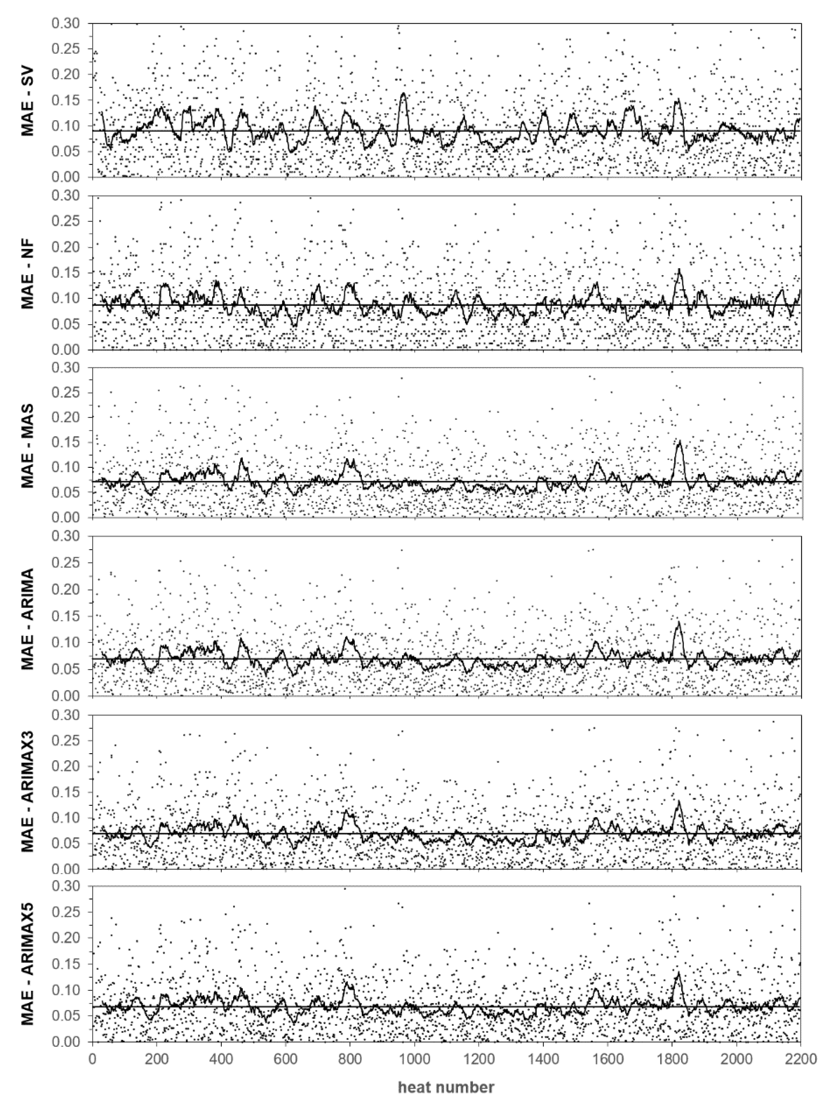
Based on the previous discussion, the optimum w values were applied to the final evaluation of each method. The resulting absolute errors are shown in Figure 9 in which each dot represents one of the 2195 heats in the test dataset. It can be seen that absolute errors are always lower than 0.3. Moreover, the daily MAE of the temperature prediction is also represented in Figure 9 with a solid curve for clarity. It can be seen that daily MAE tends to fall in the 0.05–0.15 band. The global resulting MAE is 0.0910, 0.0875, 0.0721, 0.0700, 0.0695, and 0.0685 for SV, NF, MAS, ARIMA, ARIMAX3 and ARIMAX5, corresponding to 20.0, 19.3, 15.9, 15.4, 15.3, and 15.1 °C, respectively. These values are consistent with those previously obtained during hyperparameter w optimization.
4. Discussion
4.1. Infrared Thermometry
The plant trials performed over more than 220 heats allowed to understand the connection between the IR signal and the features of the hot metal stream, while showing the feasibility of IR thermometry as hot metal temperature estimator. However, the reliability of the method, i.e., the probability of obtaining a usable output, was not higher than 60% due to the variability of stream shape and position. Regardless, since the trials were carried out under actual plant conditions, an absolute error of approximately 11 °C can be expected for such a measurement system. This temperature error corresponds to a normalized value of 0.050 as indicated by Equation (2). The adopted hot metal emissivity and IR sensor settings proved to be adequate since IR temperature estimations and actual temperatures were comparable, with the difference fully explained by a temperature drop of the hot metal in the stream. As shown in Figure 6, the departure of linear fit of IR temperature from actual values is a constant of about 50 °C, which corresponds to the expected temperature drop during hot metal pouring [21] and this was confirmed by additional measurements performed during the trial. Regarding IR device location and orientation, an 11 m height with up-down orientation was preferred for practical reasons during the trials, but a sensor placed at ground level aimed at the intrados of the stream would be a better choice. Although dust and maintenance work are expected to increase, fume and slag interferences would be greatly reduced.
4.2. Time Series Forecasting
The modeling results evidence a time component in hot metal temperatures that can be attributed to BF trends and to changes in the BF-BOF interface. These effects may propagate along time. However, time series forecasting is badly affected by missing data and other noisy factors [38]:
- Hot metal pretreatment or unexpected changes in BF-BOF interface cannot be time-predicted
- Hot metal can arrive at the BOF in different order as tapped in BF (shuffled data)
- Hot metal can arrive at the BOF from different BFs (mixed data)
- Hot metal from a BF can go to another BOF or just be poured into a pit (unnoticed missing data)
- Hot metal loaded to the BOF is actually a mix of hot metal with different process history (time averaged data)
Nevertheless, time series forecast improves temperature prediction when compared to standard value or naïve forecasting and is very easy to implement, since it only requires recalling previous temperature observations from the BOF process computer. For example, if the initially existing plant model consists of the moving average smoothing of the 20 previous temperatures, then this method results in a MAE of 0.079 that can be easily reduced to 0.072 just by changing w from 20 to 5, as shown in Figure 8. Further improvement is obtained by applying an ARIMA based model which reduces MAE to 0.069.
4.3. Combined Process and Model Development
Based on the previous results it can be realized that the different modeling and measuring approaches are not mutually exclusive but complementary [39,40]. Therefore, process and model developments can be combined for providing the BOF charge model with the best available temperature prediction at every particular process circumstance.
The main features of the involved methods are summarized in Table 3, where they are ordered by decreasing MAE but also by increasing complexity and decreasing reliability (i.e., the chances of obtaining a successful output). Attending to all these properties, the process computer will estimate a final hot metal temperature by applying each method as early as possible in the following order: SV, NF, MAS, ARIMA, ARIMAX, and IR. The final executive temperature forecast to be used by the charge model will depend on the runtime success of each method and on the moment in which the forecast is finally obtained.
The reliability, i.e., the runtime success of the modeling approach, depends mainly on the amount of required data, as evidenced by results in Table 3. The higher the number of variables and past observations required, the higher the chances of missing data. Furthermore, industrial tests of the IR approach showed that actual reliability was not much higher than 60%, as explained before.
The expected MAE of a combined procedure in which the best available method is used can be calculated as 0.0574 assuming that the reliabilities for the different methods are statistically independent: 0.0574 = 0.6 × 0.05 + (1 − 0.6) × (0.91 × 0.0685 + (1 − 0.91) × (0.92 × 0.0695 +….
The moment at which forecasts are available depends mostly on both the computing time and the earliest time at which the required input data are available. Considering that BOF time between heats is typically about 30 min and that computing time is always below 1.4 s for a regular consumer laptop, it can be concluded that computing time will not be a limiting factor. By contrast, there are relevant differences between methods regarding the earliest time at which each procedure can be applied. With the exception of the simplistic SV that is always ready, the modeling approach requires actual values of temperature and predictors from the previous heat, which are usually known about 10 min before execution of the BOF charge model for the actual heat. On the contrary, the IR method requires pouring at least part of the hot metal before running the charge model and afterwards to complete hot metal pouring and scrap preparation. In practice, this will cause a delay of 10 min or more with reference to a normal heat scheduling.
However, the strength of the combined method ensures that when a heat is scheduled with more available time, then IR temperature can be used and will overwrite the previous temperature estimation. Moreover, the actual forecast scheme is self-adaptive to changing production scenarios or even different sites. In a high production scenario, an early approximate estimate is enough, whereas in low production or hot metal shortage scenarios prediction accuracy can be improved at the tolerable cost of certain delay on BOF load preparation.
Nevertheless, any further improvement in temperature modeling will always provide additional hot metal savings. In the present study, the contribution of exogenous predictors to forecast improvement was only about 0.33 °C, much lower than expected. This low performance can be attributed to the simple way in which predictors are included in the ARIMA model. On the basis of these observations, the authors are currently researching improved modeling techniques [41], in order to expand the linear global transverse modeling of this research to a nonlinear segmented transverse modeling.
5. Conclusions
Although the evolution of hot metal temperature from BF to BOF is a complex process that cannot be accurately modeled in detail, the combined use of IR thermometry and time series forecasting allows for an improved temperature estimation that can be advantageously used in BOF charge calculation for improving cost, quality, productivity and emissions.
Simultaneous IR temperature measurement and video recording proved to be a useful method for understanding the behavior of the hot metal stream and to find the best IR settings and signal processing. The temperature measured with the IR thermometer was correlated with thermocouple measurements with a resulting MAE of 0.0500 (11 °C) with 60% of reliability.
Despite some limitations that are being addressed in the ongoing research, time series forecasting is easy to implement and provides a MAE of 0.0685–0.0721 (15–16 °C), higher than IR, but with a much better reliability of 91–98%. For these models, the moving window approach is key to gaining long-term stability without being affected by major changes in the process. Hence, modifications in the desulfurization process, or in the vessel cleaning practice, or in the insulation of torpedoes and ladles, would not affect the model performance while routine tuning of the model is not required.
The developed method can be seen as a hybrid procedure because it does not only combine sensors and modeling but also for nesting very simple models with more advanced ones. The combined model makes use of a moving window of past observations for continuous updating, and exploits the introduction of exogenous predictors for complementing the time series component. The proposed hybrid procedure has long-term stability but is also self-adaptive to varying production scenarios with an expected MAE of 0.0574 (13 °C) with 100% reliability. Therefore, the accuracy is improved by a 34%, taking Naïve Forecasting as a reference or by a 27% when compared to the initial modeling situation (MAS with w = 20).
Finally, it is necessary to further improve the regressive part of the model in order to take full advantage of the information provided by exogenous predictors. The authors are currently developing this part of the model.
Author Contributions
Conceptualization, J.D. and F.J.F.; methodology, J.D., F.J.F. and I.S.; software, J.D., F.J.F. and I.S.; validation, J.D., F.J.F. and I.S.; formal analysis, J.D. and F.J.F.; investigation, J.D.; resources, F.J.F. and I.S.; data curation, J.D.; writing—original draft preparation, J.D. and F.J.F.; writing—review and editing, J.D., F.J.F. and I.S.; visualization, J.D.; supervision, F.J.F.; project administration, J.D.; funding acquisition, F.J.F. and I.S.
Funding
This research received no external funding.
Acknowledgments
The authors would like to thank ArcelorMittal colleagues for their support and the valuable suggestions they provided. Their professional commitment has been the best stimulus for this contribution. The authors would like also to thank I. Araquistain (Land Instruments) for supporting the initial IR thermometry tests.
Conflicts of Interest
The authors declare no conflict of interest.
References
- Ghosh, A.; Chatterjee, A. Iron Making and Steelmaking: Theory and Practice; PHI Learning Pvt. Ltd.: New Delhi, India, 2008. [Google Scholar]
- Miller, T.W.; Jimenez, J.; Sharan, A.; Goldstein, D.A. Oxygen Steelmaking Processes. In The Making, Shaping, and Treating of Steel, 11th ed.; Fruehan, R.J., Ed.; The AISE Steel Foundation: Pittsburgh, PA, USA, 1998; pp. 475–524. [Google Scholar]
- Ryman, C.; Larsson, M. Reduction of CO2 emissions from integrated steelmaking by optimised scrap strategies: Application of process integration models on the BF–BOF system. ISIJ Int. 2006, 46, 1752–1758. [Google Scholar] [CrossRef]
- Ryman, C.; Larsson, M. Adaptation of process integration models for minimisation of energy use, CO2-emissions and raw material costs for integrated steelmaking. Chem. Eng. Trans. 2007, 12, 495–500. [Google Scholar]
- Jiménez, J.; Mochón, J.; de Ayala, J.S.; Obeso, F. Blast furnace hot metal temperature prediction through neural networks-based models. ISIJ Int. 2004, 44, 573–580. [Google Scholar] [CrossRef]
- Martín, R.D.; Obeso, F.; Mochón, J.; Barea, R.; Jiménez, J. Hot metal temperature prediction in blast furnace using advanced model based on fuzzy logic tools. Ironmak. Steelmak. 2007, 34, 241–247. [Google Scholar] [CrossRef]
- Jiang, Z.H.; Pan, D.; Gui, W.H.; Xie, Y.F.; Yang, C.H. Temperature measurement of molten iron in taphole of blast furnace combined temperature drop model with heat transfer model. Ironmak. Steelmak. 2018, 45, 230–238. [Google Scholar] [CrossRef]
- Sugiura, M.; Shinotake, A.; Nakashima, M.; Omoto, N. Simultaneous Measurements of Temperature and Iron–Slag Ratio at Taphole of Blast Furnace. Int. J. Thermophys. 2014, 35, 1320–1329. [Google Scholar] [CrossRef]
- Pan, D.; Jiang, Z.; Chen, Z.; Gui, W.; Xie, Y.; Yang, C. Temperature Measurement Method for Blast Furnace Molten Iron Based on Infrared Thermography and Temperature Reduction Model. Sensors 2018, 18, 3792–3806. [Google Scholar] [CrossRef]
- Pan, D.; Jiang, Z.; Chen, Z.; Gui, W.; Xie, Y.; Yang, C. Temperature Measurement and Compensation Method of Blast Furnace Molten Iron Based on Infrared Computer Vision. IEEE Trans. Instrum. Meas. 2018, 1–13. [Google Scholar] [CrossRef]
- Usamentiaga, R.; Molleda, J.; Garcia, D.F.; Granda, J.C.; Rendueles, J.L. Temperature measurement of molten pig iron with slag characterization and detection using infrared computer vision. IEEE Trans. Instrum. Meas. 2012, 61, 1149–1159. [Google Scholar] [CrossRef]
- Usamentiaga, R.; Venegas, P.; Guerediaga, J.; Vega, L.; Molleda, J.; Bulnes, F. Infrared thermography for temperature measurement and non-destructive testing. Sensors 2014, 14, 12305–12348. [Google Scholar] [CrossRef]
- Jin, S.; Harmuth, H.; Gruber, D.; Buhr, A.; Sinnema, S.; Rebouillat, L. Thermomechanical modelling of a torpedo car by considering working lining spalling. Ironmak. Steelmak. 2018, 1–5. [Google Scholar] [CrossRef]
- Nabeshima, Y.; Taoka, K.; Yamada, S. Hot metal dephosphorization treatment in torpedo car. Kawasaki Steel Tech. Rep. 1991, 24, 25–31. [Google Scholar]
- Frechette, M.; Chen, E. Thermal insulation of torpedo cars. In Proceedings of the Association for Iron and Steel Technology (Aistech) Conference Proceedings, Charlotte, NC, USA, 9–12 May 2005. [Google Scholar]
- Goldwaser, A.; Schutt, A. Optimal torpedo scheduling. J. Artif. Intell. Res. 2018, 63, 955–986. [Google Scholar] [CrossRef]
- Wang, G.; Tang, L. A column generation for locomotive scheduling problem in molten iron transportation. In Proceedings of the 2007 IEEE International Conference on Automation and Logistics, Jinan, China, 18–21 August 2007. [Google Scholar]
- Verdeja, L.F.; Barbes, M.F.; Gonzalez, R.; Castillo, G.A.; Colas, R. Thermal modelling of a torpedo-car. Rev. Metal. Madrid 2005, 41, 449–455. [Google Scholar] [CrossRef] [Green Version]
- Niedringhaus, J.C.; Blattner, J.L.; Engel, R. Armco’s Experimental 184 Mile Hot Metal Shipment. In Proceedings of the 47th Ironmaking Conference, Toronto, ON, Canada, 17–20 April 1988. [Google Scholar]
- He, F.; He, D.F.; Xu, A.J.; Wang, H.B.; Tian, N.Y. Hybrid model of molten steel temperature prediction based on ladle heat status and artificial neural network. J. Iron Steel Res. Int. 2014, 21, 181–190. [Google Scholar] [CrossRef]
- Du, T.; Cai, J.J.; Li, Y.J.; Wang, J.J. Analysis of Hot Metal Temperature Drop and Energy-Saving Mode on Techno-Interface of BF-BOF Route. Iron Steel 2008, 43, 83–86, 91. [Google Scholar]
- Liu, S.W.; Yu, J.K.; Yan, Z.G.; Liu, T. Factors and control methods of the heat loss of torpedo-ladle. J. Mater. Metall. 2010, 9, 159–163. [Google Scholar]
- Wu, M.; Zhang, Y.; Yang, S.; Xiang, S.; Liu, T.; Sun, G. Analysis of hot metal temperature drop in torpedo car. Iron Steel 2002, 37, 12–15. [Google Scholar]
- Ares, R.; Balante, W.; Donayo, R.; Gómez, A.; Perez, J. Getting more steel from less hot metal at Ternium Siderar steel plant. Rev. Metall. 2010, 107, 303–308. [Google Scholar] [CrossRef]
- Bradarić, T.D.; Slović, Z.M.; Raić, K.T. Recent experiences with improving steel-to-hot-metal ratio in BOF steelmaking. Metall. Mater. Eng. 2016, 22, 101–106. [Google Scholar] [CrossRef] [Green Version]
- Díaz, J.; Fernández, F.J. The Impact of Hot Metal Temperature on CO2 Emissions from BOF Steelmaking. Proceedings 2018, 2, 1502. [Google Scholar] [CrossRef]
- Kozlov, V.; Malyshkin, B. Accuracy of measurement of liquid metal temperature using immersion thermocouples. Metallurgist 1969, 13, 354–356. [Google Scholar] [CrossRef]
- Mazumdar, D.; Evans, J.W. Elements of mathematical modeling. In Modeling of Steelmaking Processes, 1st ed.; CRC Press: Boca Raton, FL, USA, 2010; pp. 139–173. [Google Scholar]
- Sickert, G.; Schramm, L. Long-time experiences with implementation, tuning and maintenance of transferable BOF process models. Rev. Metall. 2007, 104, 120–127. [Google Scholar] [CrossRef]
- Geerdes, M.; Toxopeus, H.; van der Vliet, C. Casthouse Operation. In Modern Blast Furnace Ironmaking: An Introduction, 1st ed.; Verlag Stahleisen GmbH: Düsseldorf, Germany, 2015; pp. 97–103. [Google Scholar]
- Williams, R.V. Control of oxygen steelmaking. In Control and Analysis in Iron and Steelmaking, 1st ed.; Butterworth Scientific Ltd.: London, UK, 1983; pp. 147–176. [Google Scholar]
- Hyndman, R.J.; Athanasopoulos, G. The forecaster’s toolbox. In Forecasting: Principles and Practice, 2nd ed.; OTexts: Melbourne, Australia, 2018; pp. 47–81. [Google Scholar]
- Papacharalampous, G.A.; Tyralis, H.; Koutsoyiannis, D. Comparison of stochastic and machine learning methods for multi-step ahead forecasting of hydrological processes. Stoch. Env. Res. Risk A 2019, 33, 481–514. [Google Scholar] [CrossRef]
- Hyndman, R.J.; Athanasopoulos, G. ARIMA models. In Forecasting: Principles and Practice, 2nd ed.; OTexts: Melbourne, Australia, 2018; pp. 221–274. [Google Scholar]
- Box, G.E.; Jenkins, G.M.; Reinsel, G.C.; Ljung, G.M. Model identification. In Time Series Analysis: Forecasting and Control, 5th ed.; John Wiley & Sons, Inc.: Hoboken, NJ, USA, 2015; pp. 179–208. [Google Scholar]
- ARIMA. Model Including Exogenous Covariates. Available online: https://es.mathworks.com/help/econ/arima-model-including-exogenous-regressors.html (accessed on 20 July 2019).
- Mihalow, F.A. Radiation thermometry in the steel industry. In Theory and Practice of Radiation Thermometry, 1st ed.; DeWitt, D.P., Nutter, G.D., Eds.; John Wiley & Sons, Inc.: Hoboken, NJ, USA, 1988. [Google Scholar]
- Tresp, V.; Hofmann, R. Nonlinear time-series prediction with missing and noisy data. Neural Comput. 1998, 10, 731–747. [Google Scholar] [CrossRef] [PubMed]
- McLean, A. The science and technology of steelmaking—Measurements, models, and manufacturing. Metall. Mater. Trans. B 2006, 37, 319–332. [Google Scholar] [CrossRef]
- Szekely, J. The mathematical modeling revolution in extractive metallurgy. Metall. Trans. B 1988, 19, 525–540. [Google Scholar] [CrossRef]
- Díaz, J.; Fernandez, F.J.; Gonzalez, A. Prediction of hot metal temperature in a BOF converter using an ANN. In Proceedings of the IRCSEEME 2018: International Research Conference on Sustainable Energy, Engineering, Materials and Environment, Mieres, Spain, 25–27 July 2018. [Google Scholar]
Figure 1.
Hot metal flow diagram inside an integrated steel mill, from blast furnace (BF) to basic-lined oxygen furnace (BOF), where the main aspects considered in this study are summarized. Hot metal sub-processes comprise BF tapping, pretreatment, transport, transfer, and BOF loading. Involved relevant variables are tapping temperature T0, final temperature T, total holding time t, desulfurization time td, empty torpedo time tc, empty ladle time tl, mi mass transferred from torpedo i, infrared sensor temperature TIR, torpedo preheating time tpc, and ladle preheating time tpl. Torpedo number nc, and ladle number nl, must be tracked in order to get their thermal histories from process databases.

Figure 2.
Hot metal transfer positions and infrared (IR) device locations used in this study. Orientations (a) and (b) were used in preliminary tests while (c) and (d) were adopted for final industrial trial. The distance between IR device and hot metal stream, and consequently sight spot diameter, are equivalent for the four options.
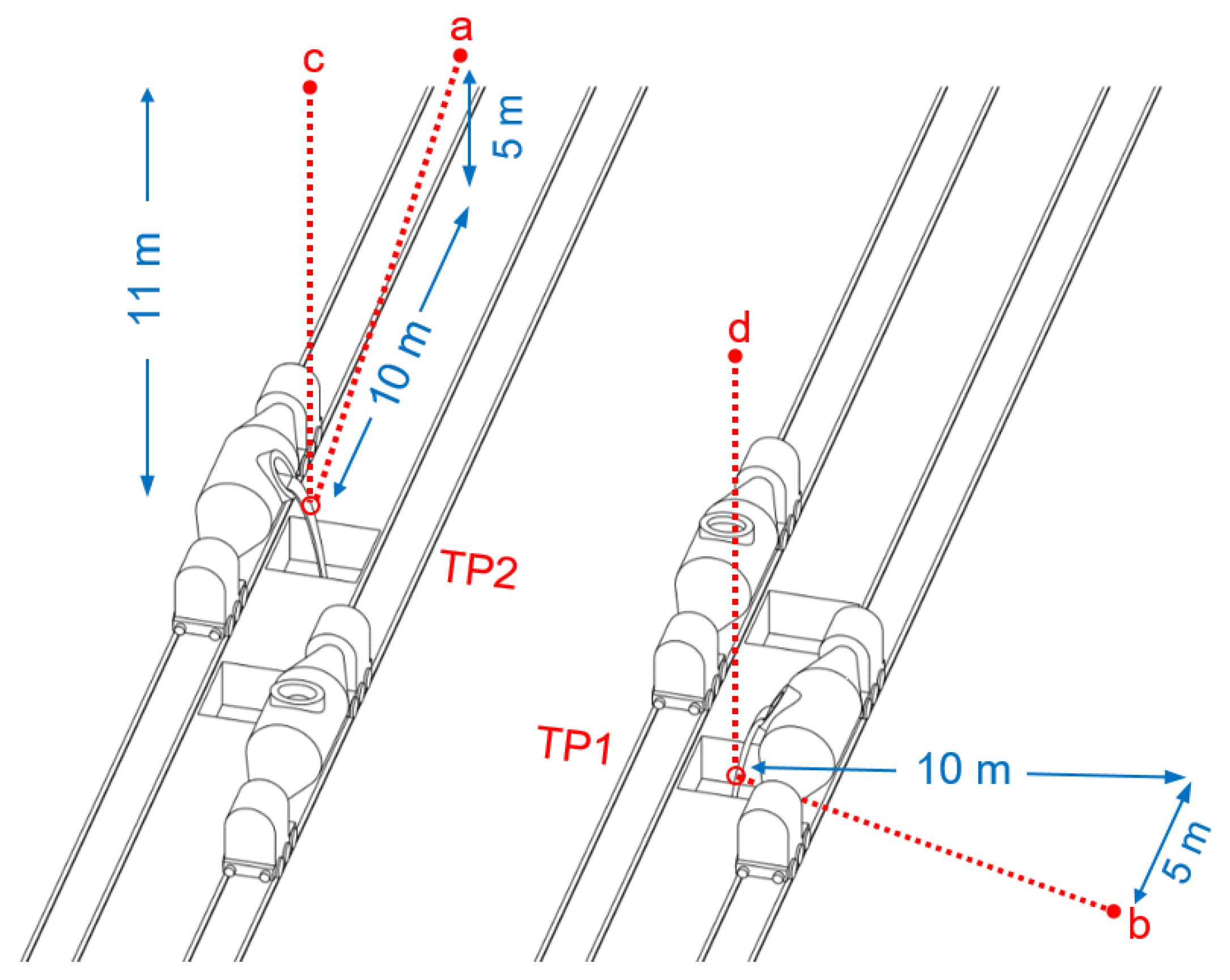
Figure 3.
IR thermometer output obtained during the pouring of 150 t of hot metal from a torpedo into a ladle. Dashed lines at 1364 and 1369 °C correspond to 85th and 95th percentile of sampled values. Letters a–j correspond to typical stream features summarized in Figure 4.
Figure 3.
IR thermometer output obtained during the pouring of 150 t of hot metal from a torpedo into a ladle. Dashed lines at 1364 and 1369 °C correspond to 85th and 95th percentile of sampled values. Letters a–j correspond to typical stream features summarized in Figure 4.

Figure 4.
Selected video frames showing relevant features of the hot metal stream as identified in Figure 3: initial narrow shape with high slag content (a), presence of liquid slag streaks (b), presence of solid slag spots (c), almost clean stream with hot metal exposed (d), final narrow shape with liquid slag streaks (e), shallow stream resulting in discontinuities (frame sequence f–j). The images were acquired through the IR device’s viewfinder in the orientation indicated as TP2-a in Figure 2. The circle in the center of the viewfinder indicates the location and size of the measurement spot.

Figure 5.
Scatterplot showing correlation between actual temperatures, and values predicted from percentile 85 (a) and percentile 95 (b) of IR thermometer readings for the first trial. Each dot corresponds to a hot metal ladle while the linear regression fit is marked with a solid line. Departure of TIR from actual values can be appreciated by referencing to the dashed line.
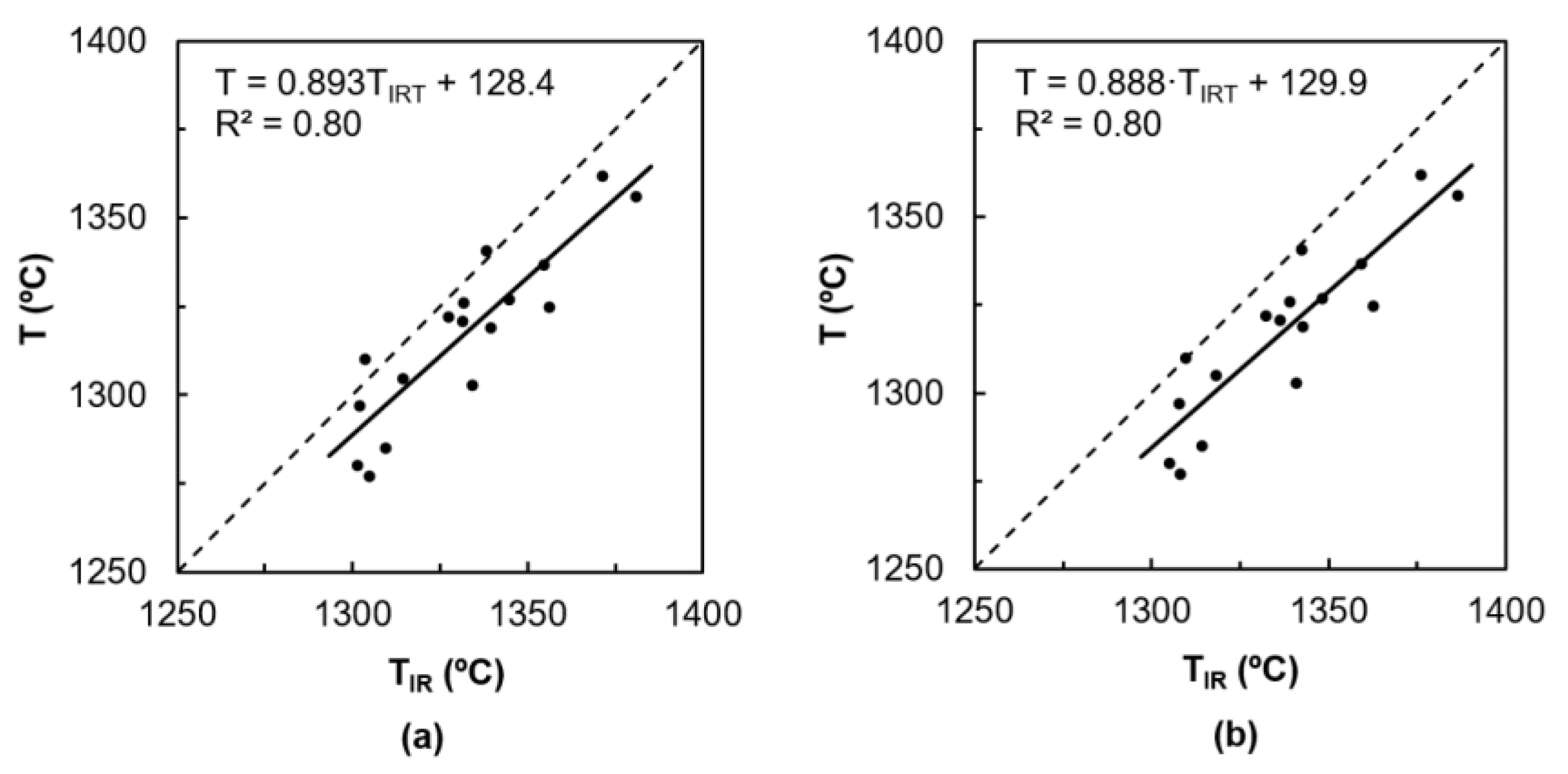
Figure 6.
Scatterplot showing the correlation between actual temperatures and values predicted from percentile 95 of IR temperature readings for the second trial, where each data point corresponds to a hot metal ladle. The two different hot metal transfer positions are represented with circles and crosses and the linear regression fit is depicted with a solid line. Departure of TIR from actual temperature values can be appreciated by referencing to the dashed line.

Figure 7.
Graphical overview of the normalized dataset used in this study which is composed of 12,195 heats (one production year). The min–max interval and the moving average for groups of 30 heats (approximately one production day) are shown for clarity. The first 10,000 heats were used for model training and testing while the last 2195 heats were used for validation of the final models.

Figure 8.
Comparison of the resulting mean absolute error (MAE) for hot metal temperature prediction as a function of the window width w, when applied to the training dataset. The lowest MAE (0.069) was obtained for moving AutoRegressive Integrated Moving Average with 5 exogenous predictors (ARIMAX5) for w above 1000 observations.
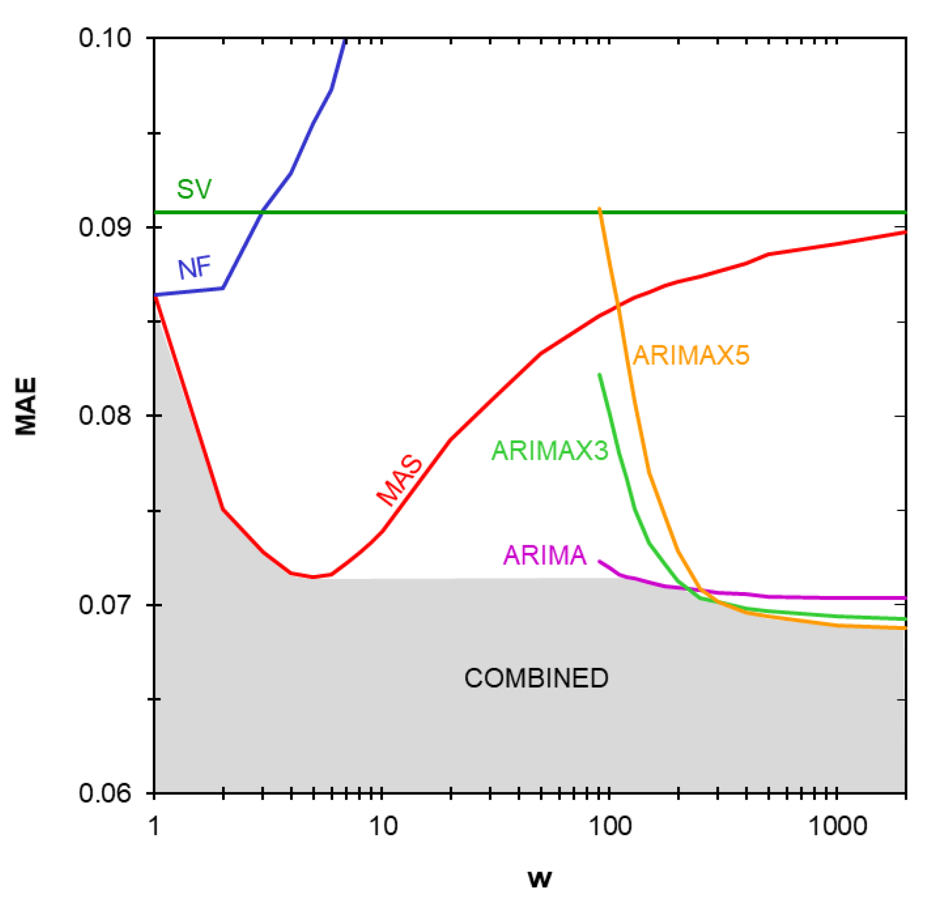
Figure 9.
Absolute errors obtained in the final testing of the six methods of temperature prediction. Each dot represents one of the 2195 heats in the test dataset. Solid curve represents the daily MAE (30 heat grouping). Solid horizontal line represents the overall MAE for SV, NF, MAS, ARIMA, ARIMAX3, and ARIMAX5 models which are 0.0910, 0.0875, 0.0721, 0.0700, 0.0695, and 0.0685, respectively.

Table 1.
Original and normalized model variables.
| Variable | Original | Normalized | |||
|---|---|---|---|---|---|
| Symbol | Min | Max | Unit | ||
| Initial temperature | T0 | 1400 | 1540 | °C | x1 |
| Elapsed time | t | 2 | 20 | h | x2 |
| Desulfurization time | td | 0 | 40 | min | x3 |
| Empty torpedo time | tc | 1 | 16 | h | x4 |
| Empty ladle time | tl | 0 | 8 | h | x5 |
| Final temperature | T | 1200 | 1420 | °C | y |
Table 2.
Optimum temperature correction coefficients for losses in torpedo and ladle, and resulting determination coefficients between TIR and T, with and without correction, when adopting different summary statistics for IR signal characterization.
Table 2.
Optimum temperature correction coefficients for losses in torpedo and ladle, and resulting determination coefficients between TIR and T, with and without correction, when adopting different summary statistics for IR signal characterization.
| Summary Statistic | CT | CL | R2 (CT, CL) | R2 (CT = 0, CL = 0) |
|---|---|---|---|---|
| Mean | 0.0 | 1.0 | 0.75 | 0.60 |
| Mode | 1.2 | 1.0 | 0.73 | 0.50 |
| Median | 0.2 | 1.5 | 0.69 | 0.47 |
| Percentile 75 | 0.9 | 0.8 | 0.77 | 0.70 |
| Percentile 85 | 1.0 | 0.9 | 0.80 | 0.70 |
| Percentile 95 | 1.0 | 0.9 | 0.80 | 0.71 |
| Maximum | 1.2 | 0.6 | 0.70 | 0.52 |
Table 3.
Main features of the studied methods for hot metal temperature estimation.
| Method | MAE | Minimum Required w | Number of Input Variables | Reliability (%) | Running Time (s) | Earliest Run in Advance (min) |
|---|---|---|---|---|---|---|
| SV | 0.0910 | 0 | 0 | 100 | - | Inf. |
| NF | 0.0875 | 1 | 1 | 99 | 0.001 | 10 |
| MAS | 0.0721 | 5 | 1 | 98 | 0.001 | 10 |
| ARIMA | 0.0700 | 100 | 1 | 95 | 0.671 | 10 |
| ARIMAX3 | 0.0695 | 250 | 4 | 92 | 1.051 | 10 |
| ARIMAX5 | 0.0685 | 300 | 6 | 91 | 1.396 | 10 |
| IR | 0.0500 | 1 | 1 | 60 | - | −10 |
© 2019 by the authors. Licensee MDPI, Basel, Switzerland. This article is an open access article distributed under the terms and conditions of the Creative Commons Attribution (CC BY) license (http://creativecommons.org/licenses/by/4.0/).
Share and Cite
MDPI and ACS Style
Díaz, J.; Fernández, F.J.; Suárez, I. Hot Metal Temperature Prediction at Basic-Lined Oxygen Furnace (BOF) Converter Using IR Thermometry and Forecasting Techniques. Energies 2019, 12, 3235. https://doi.org/10.3390/en12173235
AMA Style
Díaz J, Fernández FJ, Suárez I. Hot Metal Temperature Prediction at Basic-Lined Oxygen Furnace (BOF) Converter Using IR Thermometry and Forecasting Techniques. Energies. 2019; 12(17):3235. https://doi.org/10.3390/en12173235
Chicago/Turabian StyleDíaz, José, Francisco Javier Fernández, and Inés Suárez. 2019. "Hot Metal Temperature Prediction at Basic-Lined Oxygen Furnace (BOF) Converter Using IR Thermometry and Forecasting Techniques" Energies 12, no. 17: 3235. https://doi.org/10.3390/en12173235
Note that from the first issue of 2016, this journal uses article numbers instead of page numbers. See further details here.