Optimization of Radio Interference Levels for 500 and 600 kV Bipolar HVDC Transmission Lines ^†

Abstract

In this work, a method to compute the radio interference (RI) lateral profiles generated by corona discharge in high voltage direct current (HVDC) transmission lines is presented. The method is based on a transmission line model that considers the skin effect, through the concept of complex penetration depth, in the conductors and in the ground plane. The attenuation constants are determined from the line parameters and the bipolar system is decoupled by using modal decomposition theory. As application cases, ±500 and ±600 kV bipolar transmission lines were analyzed. Afterwards, parametric sweeps of five variables that affect the RI levels are presented. Both the RI and the maximum electric field were calculated as a function of sub-conductor radius, bundle spacing, and the number of sub-conductors in the bundle. Additionally, the RI levels were also calculated as a function of the soil resistivity, and the RIV (radio interference voltage) frequency. Following this, vector optimization was applied to minimize the RI levels produced by the HVDC lines and differences between the designs with nominal and optimal values are discussed.

1. Introduction

High voltage direct current (HVDC) transmission systems are being studied and developed in several countries around the world. In Mexico and Turkey, the future installation of HVDC transmission lines is planned because of the advantages this kind of technology presents over HVAC transmission lines, mostly in energy transmission over long distances [1]. During the design stage of an HVDC transmission system, it is necessary to carry out studies like insulation coordination, protections, and transient stability, among others [2,3,4].

Corona discharge appears at the surface of the conductors when a certain critical value of the electric field is reached, causing the ionization of the air surrounding the conductors. Some of the main consequences of corona are power loss, audible noise, and radio interference [5]. Radio interference (RI) can be any effect on the reception of a wanted radio signal due to an unwanted disturbance within the radio frequency spectrum [6]. Corona performance and radio interference are key issues during the design stage of both HVAC and HVDC transmission lines, usually as a part of electromagnetic compatibility studies (EMC) [7,8].

Concerning bipolar DC lines, corona in the positive pole is the dominant source of electromagnetic interference since the current pulses produced by this polarity have much higher amplitude than those from the negative pole. There is also a noteworthy difference between RI performance in AC and DC lines; in AC lines, the RI levels increase significantly in heavy rain weather while the RI levels in bipolar DC lines, by contrast, decrease in rain or wet snow [9,10].

There are still only a few analytical methods for calculating RI levels from DC lines, mainly due to difficulty in defining the RI excitation function through experimental studies. Based on measurements made on test lines, empirical formulas for predicting the RI levels for bipolar HVDC lines have been developed by different researching groups, some of which are described in [5,9,10]. In general, these kinds of formulas are defined for fair weather conditions, and they depend on the maximum voltage gradient, conductor diameter, and the distance between the conductor and the measuring point. Both the analytical methods presented in [5] and the empirical formulas mentioned above are only defined for horizontal configurations of bipolar lines. Also, they do not consider the soil resistivity which is a variable that affects the RI levels produced by corona in DC lines, as will be discussed later in this work.

In this paper, the computation of RI lateral profiles produced by corona discharge in HVDC transmission lines is presented. The proposed method has already been applied for calculating RI levels in HVAC lines in a previous work, where the results were very close to the measurements made on AC lines [11]. The proposed method, described in Section 2, considers a transmission line model where the skin effect is taken into consideration by using the concept of complex penetration depth in the pole conductors and in the ground plane. The soil resistivity is considered in the calculation of the complex penetration depth which, in turn, affects the series impedance of the line and the horizontal component of the magnetic field. Moreover, the attenuation constants are calculated from the line parameters and the multiconductor system is decoupled by using modal decomposition theory, which makes it possible to analyze not only horizontal bipolar lines but also any other configuration even hybrid transmission lines.

In Section 3, a comparison of computed values and measurements of RI reported in a previous publication for a DC test line of ±800 kV is also presented. In Section 4, parametric sweeps are presented in order to investigate the impacts of five important variables on RI levels and on the maximum bundle electric field. The variables are sub-conductor radius, bundle spacing, the number of sub-conductors in a bundle, soil resistivity, and the RIV (radio interference voltage) frequency.

Afterwards, Section 5 describes how vector optimization is applied in order to minimize the RI levels produced by two bipolar DC lines, one of ±500 kV and the other of ±600 kV. In the optimization study, three independent variables are considered, namely, sub-conductor radius, bundle spacing, and the number of sub-conductors in the bundle. Finally, RI lateral profiles computed with the optimal values are compared with those obtained with the nominal values.

2. Transmission Line Model for Corona Propagation Analysis

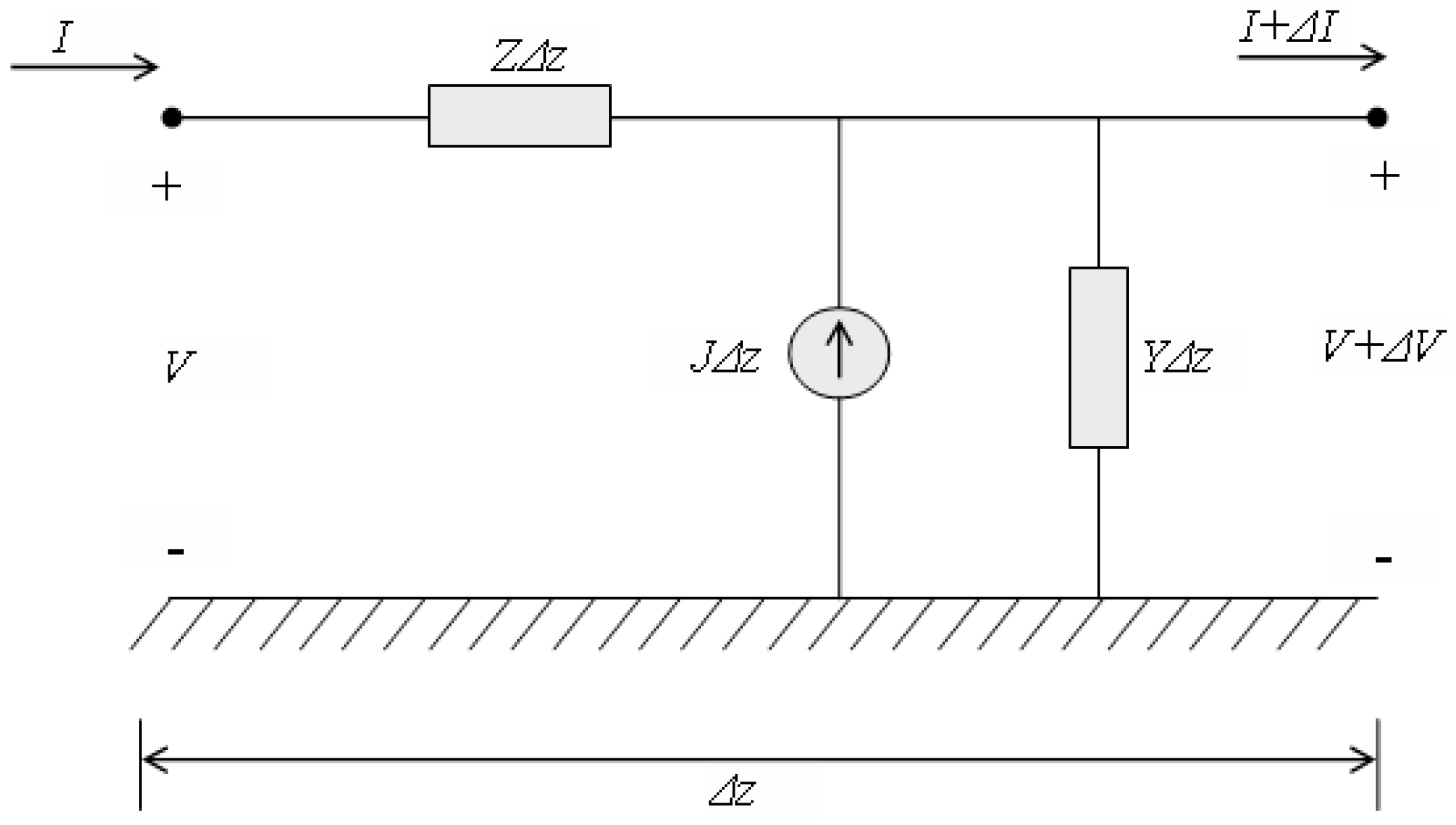
The line model used to simulate the propagation of the corona current along a multiconductor transmission line is derived from the per unit length equivalent circuit for a ∆z section, presented in Figure 1. The transmission line is considered to be infinitely long with uniform corona current density injections per unit length (J).

By applying circuit analysis, equations representing the RI propagation can be written in a matrix form including the corona current density source, as follows:

$$\frac{dV}{dz}=-ZI,$$

(1)

$$\frac{dI}{dz}=-YV+J,$$

(2)

where V and I are the voltage and the current at any point on the line, and J is the column vector of corona current densities injected into the conductors. Z and Y are square matrices that represent the series impedance and the shunt admittance per unit length of the line. These parameters are determined considering the skin effect, by using the concept of complex penetration depth in the conductors and in the ground return. They can be calculated using the formulas described in [12]. (1) and (2) represent n sets of equations for the voltage and the current for a transmission line with n pole conductors. Due to the inductive and capacitive coupling between the conductors, the n sets of equations are also coupled. The modal analysis is used to simplify Equations (1) and (2) into a number of uncoupled sets of equations which can each be solved as in the case of a single conductor line.

The modal transformation matrix M is defined by

$$\mathsf{\lambda }=M^{-1}ZYM,$$

(3)

where λ and M are the eigenvalue (diagonal) and eigenvector matrices of ZY product, respectively. The modal propagation constants Ψ and the modal attenuation constants α_m matrices are given as

$$\mathsf{\Psi }=\sqrt{\mathsf{\lambda }},$$

(4)

$${\mathsf{\alpha }}_m=\mathrm{Re}\left\{\mathsf{\Psi }\right\}.$$

(5)

The corona current density vector is obtained as

$$J=\frac{C}{2\pi {\epsilon }_0}\mathsf{\Gamma },$$

(6)

where C is the capacitance matrix of the line and Γ is the excitation function vector.

The excitation function formula obtained from [5] is

$$\Gamma ={\Gamma }_0+k_1(g_{\max }-g_0)+k_2{\log }_{10}\left(\frac{n_c}{n_0}\right)+40{\log }_{10}\left(\frac{d}{d_0}\right),$$

(7)

where:

• Γ is the RI excitation function in dB above $1\mu A/\sqrt{m}$;
• g_max is the maximum bundle electric field in kV/cm;
• n_c is the number of sub-conductors in the bundle;
• d is the sub-conductor diameter in cm;
• n₀, g₀, and d₀ are reference values given by n₀ = 6, d₀ = 4.064 cm and g₀ = 25 kV/cm.

The formula for the maximum bundle electric field for bipolar lines obtained from [13] is

$$g_{\max }=\frac{\left[1+(n_c-1)\frac{r}{R}\right]V}{n_{c}r\ln \left(\frac{2H}{{\left(n_{c}r{R}^{n-1}\right)}^{1/n}*{\left[{(2H/S)}^2+1\right]}^{1/2}}\right)},$$

(8)

where:

• V is the line to ground voltage in kV;
• r is the radius of each sub-conductor in cm;
• R is the bundle radius in cm;
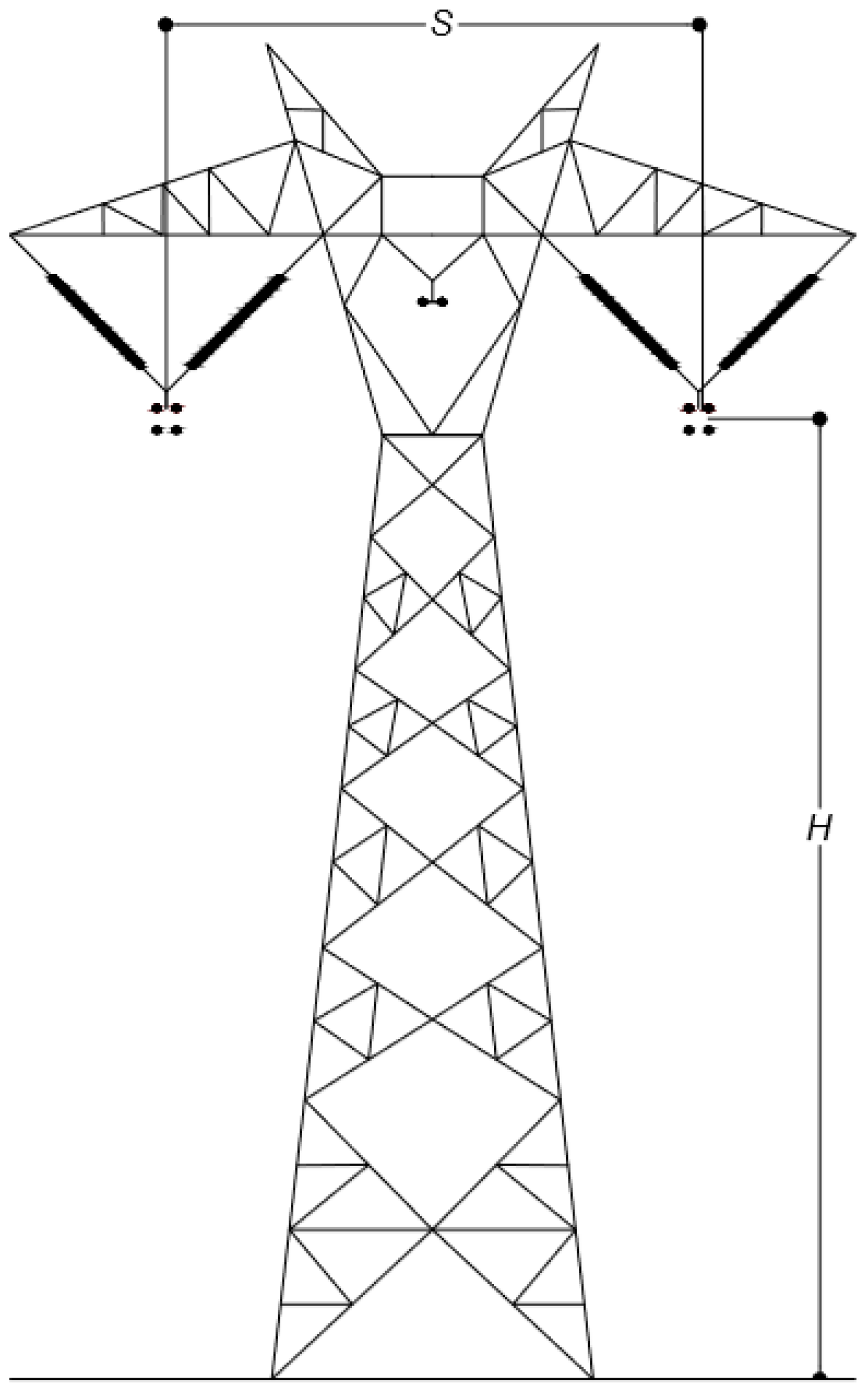
• H is the height of the poles;
• S is the distance between poles.

The reference value Γ₀ and the empirical constants k₁ and k₂ in (7) are given for all seasons in different weather conditions in [5]. Since the positive conductor of the bipolar line is considered the only source of RI, the vector Γ may be expressed as

$$\Gamma =\left[\begin{array}{c}{\Gamma }_{+}\\ 0\end{array}\right].$$

(9)

The modal corona current density vector is given by

$$J_m=M^{-1}J.$$

(10)

Using Equations (5) and (10), the modal components of current on the conductors are obtained as

$$I_m=\left[\begin{array}{c}\frac{J_{m1}}{2\sqrt{{\alpha }_{m1}}}\\ \frac{J_{m2}}{2\sqrt{{\alpha }_{m2}}}\end{array}\right],$$

(11)

where J_m1 and J_m2 are elements of the vector J_m, while α_m1 and α_m2 are the modal attenuation constants, elements of the diagonal matrix α_m. Then, the current in each conductor is obtained as

$$I=M{I}_m.$$

(12)

The current in each conductor is the sum of two modal components. By knowing the currents flowing in all the conductors of the line, the corresponding horizontal component of the magnetic field at any point (x, y) is calculated as

$$H_x={\displaystyle \sum _{i=1}^n\frac{I_i}{2\pi }}\left[\frac{h_i-y}{{(h_i-y)}^2+{(x_i-x)}^2}+\frac{h_i+y+2P}{{(h_i+y+2P)}^2+{(x_i-x)}^2}\right],$$

(13)

where:

• n is the number of poles;
• I_i is the current of the ith conductor;
• h_i is the ith conductor height;
• x_i is the ith conductor lateral distance from the center of the tower;
• x is the lateral distance of the measurement point from the center of the tower;
• y is the measurement point height above the ground;
• P is the complex depth of penetration for the ground return defined as

$$P=\sqrt{\frac{{\rho }_e}{j\omega {\mu }_e}},$$

(14)

where ρ_e and μ_e are the resistivity and permeability of the ground, respectively. The corresponding vertical component of the electric field is calculated, assuming a quasi-TEM propagation, as

$$E_y=Z_0{H}_x,$$

(15)

where the wave impedance of free space is Z₀ = 120π. After determining the electric field component, the resultant field is determined by an rms addition:

$$E_{y,total}=\sqrt{{\displaystyle \sum _{k=1}^n{\left|E_{y,k}\right|}^2}}.$$

(16)

The electric field due to corona E_y,total is usually expressed in dB above 1 μV/m using the following equation:

$$E_{y,total}(dB)=20 {\log }_{10}\frac{E_{y,total}(\mu V/m)}{1\mu V/m}.$$

(17)

3. Comparison of Measured and Computed RI Profiles of an HVDC Test Line

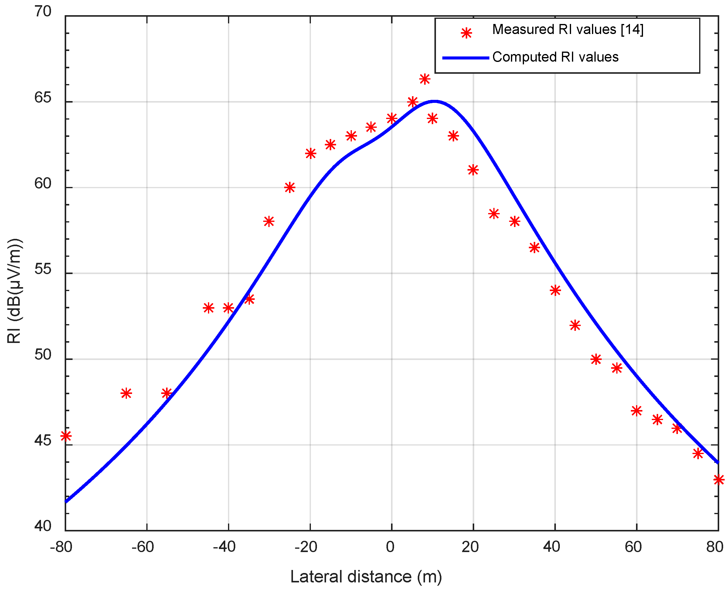
In this section, the RI values produced by an HVDC test line of ±800 kV are computed using the method described in the previous section. Then, the computed values are compared with measurements reported in [14,15]. This test line is located in the National Engineering Laboratory for UHV Technology in Kunming, China, with an altitude of 2100 m. The length of the test line is 800 m and the terminals are open ends. The measurement system consists of radio receivers connected to loop antennas with a height of 1.5 m and bandwidth of 9 kHz–30 MHz. Additionally, two wave trappers were installed between generators and the test line in order to suppress RI noises. The measuring frequency was 0.5 MHz and the measurements were made under good weather in fall. The measured RI levels are represented by quasi-peak values (QP). The data of the test line considered in the calculations are presented in

Table 1. Data of the high voltage direct current (HVDC) test line considered in the calculations.

Variable	Value
Voltage (V)	±800 kV
Number of poles (n)	2
Conductor height (H)	18 m
Distance between the poles (S)	22 m
Number of sub-conductors in the bundle (nc)	6
Bundle spacing (a)	45 cm
Sub-conductor radius (r)	1.68 cm
Ground resistivity (ρe)	100 Ωm
Measuring frequency (f)	500 kHz

.

The RI levels are given in dB with 1 μV/m as base magnitude. The profiles are plotted 80 m from each side of the center of the tower at 1.5 m above ground level. The altitude correction factor for HVDC lines proposed in [16] was applied.

In Figure 2, both measured and computed RI profiles are shown. The position zero of the horizontal axis corresponds to the center of the tower and the positive direction is towards the positive pole. It can be seen that the computed RI values are in good agreement with the measurements, principally for the measurements made on the direction of the positive pole. The maximum measured RI value is 66.3 dB while the maximum computed RI value is 65.03 dB, corresponding to a difference of 1.27 dB. Also, it can be observed the asymmetric shape of the profiles that confirms the assumption of the positive pole as the source of RI [9]. The biggest differences between measured and computed values (3–4 dB) appeared for distances longer than 60 m in the direction of the negative pole.

4. Computation of RI Levels in ±500 and ±600 kV HVDC Transmission Lines

4.1. Radio Interference Lateral Profiles

In this section, the RI lateral profiles of two bipolar HVDC transmission lines of ±500 and ±600 kV are presented. The method described in Section 2 was programmed in MATLAB in order to compute the RI levels expressed in dB with 1 μV/m as base magnitude. The RI profiles were plotted up to 50 m from each side of the center of the tower at 1 m above the ground. The tower geometry of a bipolar, quadrupole-bundle HVDC line is shown in Figure 3. Line and tower data are given in

Table 2. Data of the HVDC lines considered in the simulations.

Variable	Value
Voltage (V)	±500 or ±600 kV
Number of poles (n)	2
Conductor height of ±500 kV line (H)	27 m
Conductor height of ±600 kV line (H)	34 m
Distance between the poles (S) for both voltage levels	16 m
Number of sub-conductors in the bundle (nc)	4
Bundle spacing (a)	45 cm
Sub-conductor radius (r)	1.71 cm

.

The parameters used for the excitation formula (7) were those corresponding to fair weather condition in summer (Γ₀ = 27, k₁ = 1.83, and k₂ = 45.8), which is assumed to be the most critical condition for the generation of radio interference voltages in HVDC lines [5]. In the simulations, ground resistivity was considered with a value of 100 Ωm, and the RIV frequency was taken as 0.5 MHz, the frequency that is usually considered in the RI measurements [15,17].

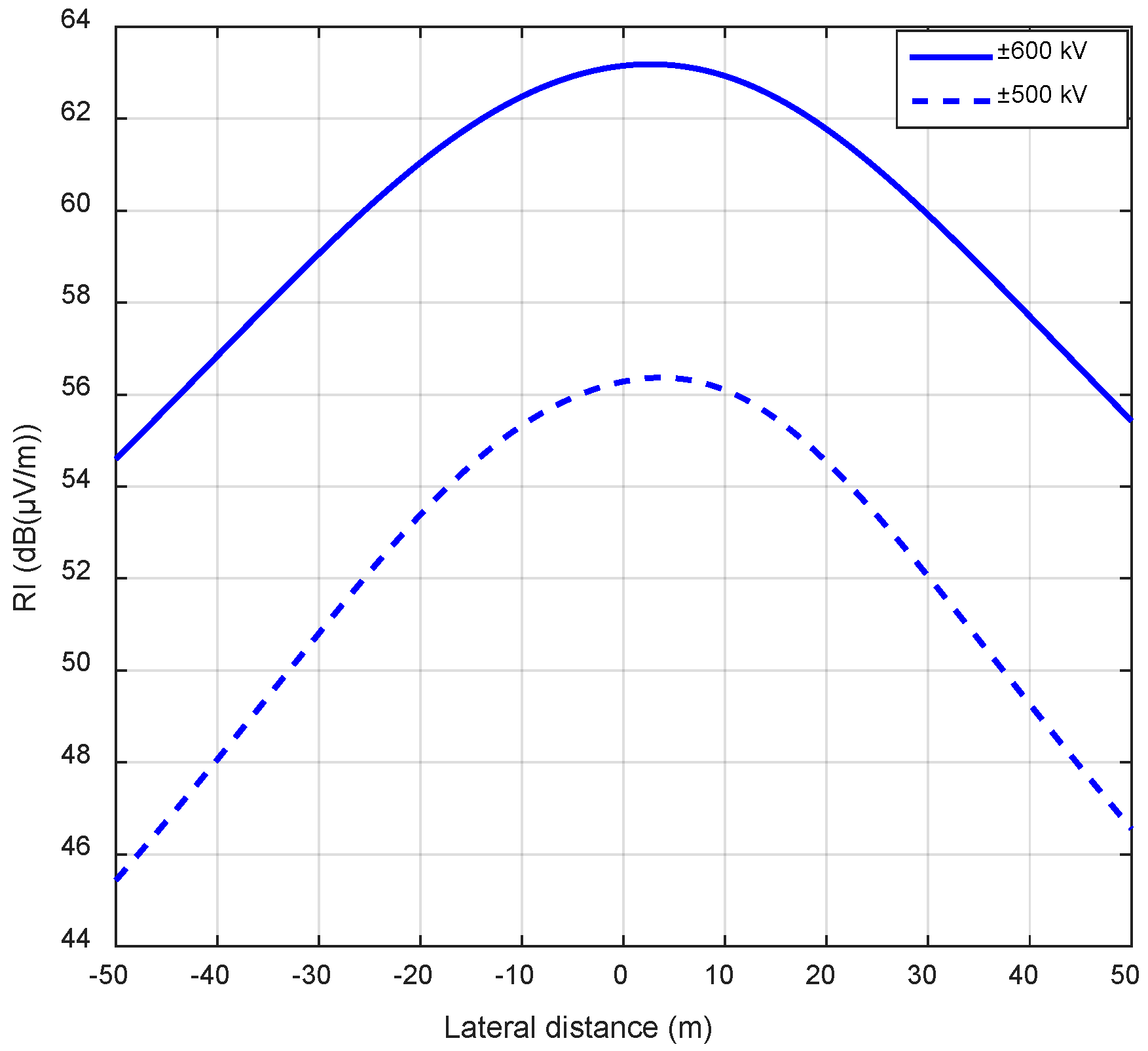
Simulated RI lateral profiles at rated conditions are shown in Figure 4 for both HVDC lines. The zero position of the horizontal axis corresponds to the center of the tower and the positive direction is towards the positive pole. The maximum values of RI for the bipolar lines of ±500 and ±600 kV are 56.37 and 63.19 dB, respectively.

As can be seen in Figure 4, the maximum values of RI are placed closer to the positive pole because of the higher amplitude of the positive streamers in comparison with the Trichel pulses in negative polarity. In fact, the streamer pulses from positive corona are considered as the dominant source of the RI in DC transmission lines [9].

Some details of the calculations are summarized in

Table 3. Results of the calculations for the bipolar HVDC lines.

Variable	Line of ±500 kV	Line of ±600 kV
Maximum bundle electric field (gmax)	19.93 kV/cm	23.83 kV/cm
Excitation function (Γ)	6.65 dB	13.79 dB
Maximum value of RI	56.37 dB	63.19 dB
RI at point (x, y) = (23 m, 1.0 m)	53.85 dB	61.27 dB

. Note that an additional measurement at a reference point (x, y) = (23 m, 1.0 m) is included in the table, and this value will be used for comparisons in the parametric sweep computations presented in the next section.

4.2. Parametric Sweeps

In this section, parametric sweeps of five variables that affect the RI levels are presented. Both the RI and the maximum bundle electric field (g_max) are calculated as a function of sub-conductor radius, bundle spacing, and the number of sub-conductors in the bundle and, additionally, the RI levels are also calculated as a function of the soil resistivity and RIV frequency. In the parametric sweeps, the reported RI level was computed considering a measurement point at (x, y) = (23 m, 1.0 m). The previous consideration is taken according to the Canadian Standards Association that specifies tolerable limits for RI in a reference point placed at 15 m from the outermost conductor of the power line [18]. For this case, the reference point is assigned as (23 m, 1.0 m), i.e., 23 m from the center of the tower and 1 m above the ground.

In Figure 5, it can be seen that both the RI and the maximum bundle electric field (g_max) tend to decrease as the sub-conductor radius increases. This behavior is observed for the two voltage levels, however, the decrease rate becomes smaller as the sub-conductor radius increases. Therefore, the sub-conductor radius is determined according to some other technical and economic considerations [1].

Figure 6 shows the impact of bundle spacing on RI and g_max values. At first glance, the RI levels present a minimum for a bundle spacing around 30 cm; whereas the optimum bundle spacing for g_max (with a minimum value) is between 30 and 40 cm. This behavior shows that the bundle spacing is a critical variable for RI and g_max levels. Therefore, it should be selected carefully around the aforementioned optimal values while taking into account some other technical and constructional constraints.

Simulation results show that the RI levels go through a minimum value for a certain number of conductors in the bundle (Figure 7a), whereas g_max decreases continuously with the increment in the number of conductors in the bundle (Figure 7b). The lowest RI value for the ±500 and ±600 kV lines are achieved with five and six sub-conductors in a bundle, respectively. The sensitivity of RI levels to the number of conductors in the bundle is lower around the optimal point in the ±600 kV lines, which provides flexibility in the choice of the number of conductors. In fact, the increment in the RI levels—observed when the number of sub-conductors in a bundle is higher than six—can be due to the reference value of n₀ = 6 used in the excitation function. It is clear that the third term in Equation (7) becomes positive for values of n_c greater than 6.

The effect of soil resistivity on RI levels is illustrated in Figure 8. The RI levels show a minimum for a soil resistivity value between 2000 and 5000 Ωm for both systems. The maximum bundle electric field, g_max, is not dependent on the soil resistivity.

Finally, the impact of RIV frequency on RI levels is illustrated in Figure 9. It can be seen how the RI values tend to decrease while the measuring frequency increases. This behavior is attributed to the increment in the modal attenuation constants with the frequency. g_max is not a function of the RIV frequency.

According to the aforementioned results, it seems that an optimum HVDC line design can be obtained by varying the geometrical dimensions. Both the soil resistivity and the measurement frequency are not considered adjustable parameters during the design process; therefore, they are not included in the optimization process that is presented below.

5. Optimization of Radio Interference Levels in HVDC Lines

In this section, vector optimization is applied in order to minimize the RI levels produced by each of the two HVDC lines described in the previous section. Only the three geometric parameters—sub-conductor radius, bundle spacing, and the number of sub-conductors in a bundle—are taken into account in the optimization process. The genetic algorithm solver of the MATLAB optimization toolbox is used. The RI value at the reference point (x, y) = (23 m, 1.0 m) is considered as the objective function. In

Table 4. Genetic algorithm parameters for the MATLAB optimization toolbox.

Parameter	Value
Population type	Double vector
Population size	100
Scaling function	Rank
Selection function	Stochastic uniform
Elite count	1.5
Crossover fraction	0.8
Mutation function	Constraint dependent
Crossover function	Constraint dependent
Migration direction	Forward
Migration fraction	0.2
Migration interval	20
Constraint initial penalty	10
Constraint penalty factor	100

, the parameters used in the optimization process for both ±500 and ±600 kV lines are shown.

Based on the previous simulations, lower and upper limits are specified for each independent geometric variable. Optimization results are presented together with the variable limits in

Table 5. Optimal geometric parameters for ±500 kV HVDC line.

Variable	Lower Bound	Upper Bound	Nominal Value	Optimal Value
Sub-conductor radius	1.04 cm 477 MCM	2.21 cm 2167 MCM	1.71 cm 1272 MCM	2.21 cm 2167 MCM
Bundle spacing	20 cm	80 cm	45 cm	42 cm
Number of sub-conductors	2	8	4	3
RI at (x, y) = (23 m, 1.0 m)			53.85 dB	50.23 dB
Total mass of the bundle			4 × 2135 = 8540 kg/km	3 × 3431 = 10,293 kg/km

and

Table 6. Optimal geometric parameters for ±600 kV HVDC line.

Variable	Lower Bounds	Upper Bounds	Nominal Values	Optimal Values
Sub-conductor radius	1.04 cm 477 MCM	2.21 cm 2167 MCM	1.71 cm 1272 MCM	2.21 cm 2167 MCM
Bundle spacing	20 cm	80 cm	45 cm	38 cm
Number of sub-conductors	2	8	4	4
RI at (x, y) = (23 m, 1.0 m)			61.27 dB	58.88 dB
Total mass of the bundle			4 × 2135 = 8540 kg/km	4 × 3431 = 13,724 kg/km

for the ±500 and ±600 kV HVDC lines, respectively.

According to the optimization results shown in Table 5 for the ±500 kV line, increasing the sub-conductor radius from 1.71 to 2.21 cm, reducing the bundle spacing from 45 to 42 cm, and reducing the number of sub-conductors from 4 to 3, the RI value calculated at the reference point (x, y) = (23 m, 1.0 m) is reduced from 53.85 dB with the nominal parameters to 50.23 dB with the optimal parameters. In Figure 10, the comparison of nominal and optimized RI lateral profiles for the ±500 kV line is shown. An almost constant reduction of 3.62 dB can be observed along the complete profile. Due to the increment in the sub-conductor radius, the total mass of the bundle increased from 8540 to 10,293 kg/km. The increment of 1753 kg/km should be evaluated from an economical point of view as well as from the strength of the tower to support this new load.

According to the optimization results for the ±600 kV line shown in Table 6, by increasing the sub-conductors radius from 1.71 to 2.21 cm, reducing the bundle spacing from 45 to 38 cm, and keeping the number of sub-conductors as 4, the RI value computed at the measuring point was reduced from 61.27 dB for the nominal parameters to 58.88 dB for the optimal parameters. In Figure 11, the comparison of nominal and optimized RI lateral profiles for the ±600 kV line is shown. The increment in the sub-conductor radius produces an increment in the total mass of the conductor bundle from 8540 to 13,724 kg/km. Similar to the ±500 kV line case, the increment of 5184 kg/km should be evaluated from the economical and mechanical point of view.

6. Discussion

With regard to the ±500 kV line, it is observed that this line presents an RI level (53.85 dB) below the maximum tolerable limit recommended by the relevant standards, which is usually 60 dB in the reference measuring point [18]. Nevertheless, optimization studies, such as the one applied in this case, allow for maintaining an acceptable RI performance of the line at even higher altitude regions. Considering an RI altitude correction factor of 1 dB/300 [19], the initial HVDC line design would exceed 60 dB at an altitude of 1900 m above the sea level; however, with the optimization applied, this line would present an acceptable RI performance (59.23 dB) until 2700 m above the sea level. On the other hand, even though the number of sub-conductors was reduced from 4 to 3, because of the increment in the sub-conductor radius, the total mass of the bundle increased from 8540 kg/km to 10,293 kg/km. This increment of 1753 kg/km (20.5%) in the total mass of the bundle should be evaluated from an economic point of view as well as from the strength of the tower to support this new load [20,21].

Regarding the ±600 kV HVDC transmission line, the RI value computed at the reference point (23 m, 1.0 m) is 61.27 dB, exceeding the limit of 60 dB for this voltage level. With the adjustments in the sub-conductor radius and bundle spacing derived from the optimization study, the RI value was reduced to 58.88 dB. This optimal case involves the use of larger conductors, increasing the total mass of the conductors by 5184 kg/km (60.7%), therefore, for this option, the adjustments derived from the optimization study seem to be feasible only in those cases that consist in the conversion of an AC line to DC operation, where one of the phases is removed.

In future work, it would be interesting to consider other variables, such as the height and the distance between the poles, a comparison of different configurations of the line (horizontal and vertical), and the inclusion of shielding wires in the model. Also, to determine the feasibility of the increment of the sub-conductor radius, it is necessary to consider the maximum mass that the towers can support as a constraint in the optimization study.

7. Conclusions

Radio interference lateral profiles in HVDC lines were computed using a method that considers a transmission line model which includes the skin effect in the conductors and in the ground plane. The attenuation constants were determined from the line parameters, and the bipolar system is decoupled using modal decomposition theory. As application cases, two HVDC bipolar transmission lines were analyzed, one of ±500 kV and the other of ±600 kV. The parametric sweeps of five prospective parameters revealed that, as expected, the RI levels decrease when increasing the sub-conductor radius. However, in the case of bundle spacing and the number of sub-conductors, the results show that these parameters should be carefully selected because these present a more complicated relationship with the magnitude of the RI level. Finally, vector optimization was applied to minimize RI levels and the feasibility of the obtained optimal designs discussed. This kind of electromagnetic compatibility study (EMC) can be used to estimate the magnitude of the impact on the environment in the vicinity of a transmission line during the design stage.

References

- Font, A.; Ilhan, S.; Ismailoglu, H.; Espino-Cortes, F.P.; Ozdemir, A. Design and Technical Analysis of 500–600 kV HVDC Transmission System for Turkey. In Proceedings of the 10th International Conference on Electrical and Electronics Engineering ELECO 2017, Bursa, Turkey, 30 November–2 December 2017. [Google Scholar]
- Rodrigues, E.; Pontes, R.S.T.; Bandeira, J.; Aguiar, V.P.B. Analysis of the Incidence of Direct Lightning over a HVDC Transmission Line through EFD Model. Energies 2019, 12, 555. [Google Scholar] [CrossRef]
- Pei, X.; Tang, G.; Zhang, S. A Novel Pilot Protection Principle Based on Modulus Traveling-Wave Currents for Voltage-Sourced Converter Based High Voltage Direct Current (VSC-HVDC) Transmission Lines. Energies 2018, 11, 2395. [Google Scholar] [CrossRef]
- Naeem, R.; Cheema, M.S.; Ahmad, M.; Haider, S.A.; Shami, U.T. Impact of HVDC grid segmentation topology on transient stability of HVDC-segmented electric grid. In Proceedings of the 2015 International Conference on Open Source Systems & Technologies (ICOSST), Lahore, Pakistan, 17–19 December 2015; pp. 132–136. [Google Scholar]
- Maruvada, P.S. Corona Performance of High-Voltage Transmission Lines; Research Studies Press Ltd.: Baldock, UK, 2000. [Google Scholar]
- Electric Power Transmission and the Environment: Fields, Noise and Interference. In CIGRE Technical Brochure; No. 74; National Grid Research and Development Centre: Paris, France, 2000.
- Tejada-Martinez, C.; Espino-Cortes, F.P.; Ilhan, S.; Ozdemir, A. Computation of Corona Radio Interference Levels in HVDC Transmission Lines. In Proceedings of the 10th International Conference on Electrical and Electronics Engineering ELECO 2017, Bursa, Turkey, 30 November–2 December 2017. [Google Scholar]
- Tejada-Martinez, C.; Espino-Cortes, F.P.; Ilhan, S.; Ozdemir, A. Optimization of Corona Radio Interference Levels in HVDC Transmission Lines. In Proceedings of the 2018 International Conference on High Voltage Engineering and Application, ICHVE 2018, Athens, Greece, 10–13 September 2018. [Google Scholar]
- Interferences Produced by Corona Effect of Electric Systems. In CIGRE Technical Brochure; No. 61; CIGRE Committee Report: Paris, France, 1996.
- Impacts of HVDC Lines on the Economics of HVDC Projects. In CIGRE Technical Brochure; No. 388; Task Force: Paris, France, 2009.
- Tejada-Martinez, C.; Gómez, P.; Escamilla, J.C. Computation of Radio Interference Levels in High Voltage Transmission Lines with Corona. IEEE Lat. Am. Trans. 2009, 7, 54–61. [Google Scholar] [CrossRef]
- Paul, C.R. Analysis of Multiconductor Transmission Lines, 2nd ed.; Wiley-Interscience: New York, NY, USA, 2008. [Google Scholar]
- Padiyar, K.R. HVDC Power Transmission Systems: Technology and System Interactions; Wiley: New York, NY, USA, 1990. [Google Scholar]
- Tian, F.; Yu, Z.; Zeng, R. Radio Interference and Audible Noise of the UHVDC test line under high altitude condition. In Proceedings of the 2012 Asia-Pacific Symposium on Electromagnetic Compatibility, Singapore, 21–24 May 2012; pp. 449–452. [Google Scholar]
- Yu, Z.; Zeng, R.; Li, M.; Li, R.; Liu, L.; Yang, D.; Zhang, Z.; Zhang, B.; Tian, F. Radio Interference of Ultra HVDC Transmission Lines in High Altitude Region. In Proceedings of the 2010 Asia-Pacific International Symposium on Electromagnetic Compatibility, Beijing, China, 12–16 April 2010; pp. 1672–1675. [Google Scholar]
- Zhao, L.; Cui, X.; Xie, L.; Lu, J.; He, K.; Ju, Y. Altitude Correction of Radio Interference of HVdc Transmission Lines Part II: Measured Data Analysis and Altitude Correction. IEEE Trans. Electromagn. Compat. 2017, 59, 284–292. [Google Scholar] [CrossRef]
- Baoquan, W.; Dichen, L.; Xiong, W.; Yao, L. The study on the radio interference from ±800kV Yun Guang UHVDC transmission line. In Proceedings of the 2006 International Conference on Power System Technology, Chongqing, China, 22–26 October 2006; pp. 1–5. [Google Scholar]
- Limits and Measurement Methods of EM Noise from AC Power Systems, 0.15–30 MHz; Standard CAN3-C108.3.1-M84; Canadian Standard Association: Toronto, ON, Canada, 2014.
- IEC TR, CISPR 18-3, Radio Interference Characteristics of Overhead Power Lines and High Voltage Equipment—Part 3: Code of Practice for Minimizing the Generation of Radio Noise; IEC: Geneva, Switzerland, 2010; pp. 30–31.
- Yang, J.; Wu, J.; Li, M.; Han, J. Structural Optimization for the China UHV Transmission Steel Tower. In Proceedings of the 2010 Asia-Pacific Power and Energy Engineering Conference, Chengdu, China, 28–31 March 2010; pp. 1–4. [Google Scholar]
- Vivek, K.S.; Nagendra, V. Optimized Design of Steel Transmission Line Tower by Limit State Methodology. Int. J. Mod. Eng. Res. IJMER 2015, 5, 81–100. [Google Scholar]
Figure 1.
Per unit length equivalent transmission line circuit with corona.
Figure 2.
Comparison of measured [14] and computed radio interference (RI) profiles.
Figure 3.
Tower geometry of a bipolar HVDC transmission line.
Figure 4.
RI lateral profiles of the two HVDC transmission lines.
Figure 5.
Parametric sweeps: (a) RI as a function of sub-conductor radius; (b) Maximum bundle electric field (gmax) as a function of sub-conductor radius.
Figure 6.
Parametric sweeps: (a) RI as a function of bundle spacing; (b) Maximum bundle electric field (gmax) as a function of bundle spacing.
Figure 7.
Parametric sweeps: (a) RI as a function of the number of sub-conductors in the bundle; (b) Maximum bundle electric field (gmax) as a function of the number of sub-conductors in the bundle.
Figure 8.
RI as a function of the soil resistivity.
Figure 9.
RI as a function of the RIV frequency.
Figure 10.
Comparison of nominal and optimized RI lateral profiles for ±500 kV line.
Figure 11.
Comparison of nominal and optimized RI lateral profiles for ±600 kV line.