Can Nighttime Light Data Be Used to Estimate Electric Power Consumption? New Evidence from Causal-Effect Inference

Abstract

Nighttime light data are often used to estimate some socioeconomic indicators, such as energy consumption, GDP, population, etc. However, whether there is a causal relationship between them needs further study. In this paper, we propose a causal-effect inference method to test whether nighttime light data are suitable for estimating socioeconomic indicators. Data on electric power consumption and nighttime light intensity in 77 countries were used for the empirical research. The main conclusions are as follows: First, nighttime light data are more appropriate for estimating electric power consumption in developing countries, such as China, India, and others. Second, more latent factors need to be added into the model when estimating the power consumption of developed countries using nighttime light data. Third, the light spillover effect is relatively strong, which is not suitable for estimating socioeconomic indicators in the contiguous regions between developed countries and developing countries, such as Spain, Turkey, and others. Finally, we suggest that more attention should be paid in the future to the intrinsic logical relationship between nighttime light data and socioeconomic indicators.

1. Introduction

In the field of the social sciences, we often use secondhand data released by the government or research institutions. When studying smaller administrative units, data are often not available. Meanwhile, data are often not timely, and their time span is often large [1]. Croft discovered that nighttime light data can be used as an indicator of human activities [2]. Recently, scientists began to use remote sensing data to estimate the data of social activities. Among these, the nighttime lighting data released by the U.S. National Oceanic and Atmospheric Administration (NOAA) is the most used. The data were collected by the Operational Linescan System (OLS) flown by the U.S. Air Force Defense Meteorological Satellite Program (DMSP) from 1992 to 2012. In 2013, Visible Infrared Imaging Radiometer Suite (VIIRS) data products replacing the DMSP and OLS appeared, with higher resolution and grayscale, effectively avoiding pixel mutation and saturation, and eliminating the interference of stray light, lightning, moonlight, and cloud cover [3].

Nighttime light data are an important symbol of human activity, and they are also the most direct feature of the urbanization of human society in the spatial dimension. The multidimensional and multiscale study of global and regional nighttime light data is helpful to understand the connection between global environmental change and the human environment. In recent years, nighttime light data have been increasingly used to aid the rapid assessment and comprehensive spatial analysis of key elements of urbanization, such as urban land cover, population estimates, and economic activity at global or regional scales [4]. Because of their global extent and standardized production and the relative ease with which DMSP nighttime light data can be accessed, they have been widely used as a proxy for other more difficult means of measuring these economic and social indicators [5]. The logic is that urban processes are highly correlated with each other [6]; if one process or activity can be measured well, it can be used to make reasonable estimates of others. In the existing research, the methods of estimation are linear regression, logic regression, and power regression. Finally, these models can achieve a very high coefficient of determination or coefficient of correlation. Some of them can reach 99%. However, this is also a signal of spurious regression in econometrics. Therefore, we want to know whether there is a causal relationship between nighttime light data and these social indexes, from the perspective of econometrics.

In this paper, we propose a causal-effect inference method to test whether nighttime light data is suitable to estimate socioeconomic indicators and select electric power consumption as the research object, and use econometric methods to test the relationship between nighttime light data and electric power consumption on a country level. First, in Section 2 we summarize the research results of estimating electric power consumption using light data. Then we introduce data resources and research objects, including countries and time span. The testing process is described in Section 3. The empirical results are shown in Section 4. In Section 5, we discuss the empirical results. Finally, the conclusions and suggestions are made in Section 6.

2. An Overview of the Literature

Nighttime lights have been used to map economic activity [7,8,9,10,11], energy production [12,13], energy consumption [14,15,16,17,18,19,20,21,22], carbon emissions [23,24,25,26,27], stocks of metals [28,29,30,31,32,33], and PM2.5 [34]. Research areas include the world, a particular region, or a specific country. Spatial scales include national, provincial, municipal, or even smaller ones. Estimation methods include linear regression, logical regression, and power regression [35]. These papers are summarized in

Table 1. Summary of nighttime light data application.

Authors	Objects	Region	Scale	Methods
Henderson et al. [9]	GDP	World	Country	Linear regression
Shi et al. [8]	GDP and electric power consumption	China	Province	Linear regression
Zhang and Seto [10]	Urbanization	India, China, Japan, and the United States	Country	Linear regression
Ma et al. [11]	Urbanization	China	City	Linear regression
Elvidge et al. [12]	Energy production	World	Country	Linear regression
Do et al. [13]	Energy production	Islamic State	Country	Linear regression
Letu et al. [21]	Energy production	13 Asian countries	Country and city	Cubic regression
Xiao et al. [14]	Energy consumption	China	Province	Spatiotemporal Geographically weighted regression
Shi et al. [16]	Energy consumption	the Belt and Road countries	Country	Power regression
He et al. [22]	Energy consumption	China	Province	Linear regression
Meng et al. [27]	Carbon emissions	China	City	Linear regression
Shi et al. [23]	Carbon emissions	China	Province	Panel econometrics
Shi et al. [25]	Carbon emissions	China	Country	Linear regression
Takahashi et al. [33]	Metal stock	Asian countries	Country	Linear regression
Hattori et al. [30]	Metal stock	World	Country	Linear regression
Liang et al. [28]	Metal stock	China	Province	Logistic regression
Liang et al. [29]	Metal stock	World	Country	Linear regression
Ji et al. [34]	PM 2.5	China	Province	Linear regression

.

Nighttime light intensity data were first used to estimate population, GDP, and electric power consumption [4,36,37]. It is important to test a regression model based on some information criteria, such as AIC, BIC, and so on. However, they did not care about these information criteria in existing papers except R Square. They made the prediction based on a high adjusted R Square. An adjusted R Square is the most important criterion. It is safe to interpret night lights as an indication of anthropogenic activity specifically attributable to the use of electric lighting. In previous years, due to the lack of statistical data, some scholars used light data to estimate energy consumption in poor countries and regions [4,12,13]. With the improvement of statistical data at the national level, scholars began to use light data to estimate the energy consumption of city-level or smaller units, mainly electric power consumption [8,14,20,22]. According to the existing literature, the relationship between nighttime light intensity and electric power consumption is the earliest and most studied. Therefore, we choose electric power consumption as the research object of this paper. The research process proposed in this paper can be used to test other objects, such as GDP, metal stocks, carbon emissions, and so on.

3. Materials and Methods

3.1. Method

A causal-effect inference method is proposed, and three kinds of econometric and statistical analysis will be performed, namely correlation analysis, cluster analysis, and causality analysis. First, we conducted correlation analyses on the time and space dimensions. Meanwhile, based on the results of the spatial dimension correlation analysis, a clustering analysis of samples was carried out. Then, we selected three kinds of panel data analysis methods: A panel unit root test [37,38,39,40], a panel cointegration test [40,41], and a panel causality test [42,43,44]. The test process can be seen in Figure 1 and contains seven steps in total. The software of the test process is mainly R and ArcGIS in this paper.

Step 1: First of all, we collected data of socioeconomic indicators from released statistical databases. Meanwhile, nighttime light data were downloaded from the NOAA website. According to the spatial scale of the socioeconomic indicators, the pre-processing of the nighttime light data was carried out. For example, if we all collect national annual data, the lighting data should also be aggregated into the national annual level (Equation (1)):

$$Nightligh{t}_{year}={\displaystyle \sum }_{i=1}^{n}nightligh{t}_i$$

(1)

Step 2: We calculated the correlation coefficient and tested spatial dependence between the two series. First, we calculated the annual correlation coefficient by using annual data from countries (Equation (2)). Then we used annual data from each country to calculate the country’s own correlation coefficient (Equation (3)). Then, the correlation results were analyzed.

$$R_t\left(X_t,Y_t\right)=\frac{Cov\left(X_t,Y_t\right)}{\sqrt{Var\left[X_t\right]Var\left[Y_t\right]}}$$

(2)

$$R_i\left(X_i,Y_i\right)=\frac{Cov\left(X_i,Y_i\right)}{\sqrt{Var\left[X_i\right]Var\left[Y_i\right]}}$$

(3)

where in Equations (2) and (3), Cov and Var represent the covariance matrix and the variance, respectively; R_t denotes the correlation coefficient between X and Y at time t; X_t denotes the data set vector of variable X at time t; Y_t denotes the data set vector of variable Y at time t; R_i denotes the correlation coefficient of the i-th country; X_i denotes the data set vector of the i-th country’s variable X; and Y_t denotes the data set vector of the i-th country’s variable Y.

Step 3: Meanwhile, we firstly tested the spatial dependence of the correlation coefficients based on spatial statistic methods [45]. The method for spatial dependence testing was GW statistics in this paper [46]. This step was optional. If it was independent of the spatial dimension, we jumped to Step 4. If there was spatial dependence, we needed to classify them. There are many methods of spatial clustering analysis. Which method to choose depended on the results of the correlation analysis. In this paper, we conducted a cluster analysis of the spatial dimension using a natural breaks classification method based on the GW correlation coefficient [46,47]. The number of clusters was determined by the algorithm itself. In all the next steps, we examined the whole sample and each cluster separately.

Step 4: Stationarity or cointegration is necessary for a causality test [44]. In the test process of non-stationarity panel data, Levin and Lin found that the limit distribution of these estimators must obey a Gaussian distribution. These results were also applied to heterogeneous panel data, and an early version of the panel unit root test was established. Later, after improvements by Levin et al., the Levin Lin and Chu (LLC) method of checking the unit root of the panel was put forward [39]. Levin et al. pointed out that this method allows for different intercepts and time trends, heteroscedasticity, and high-order series correlation, and is suitable for a panel unit root test for medium dimensions (time series between 25 and 250, cross-sectional numbers between 10 and 250). Lm et al. also proposed the Im Pesran and Shin (IPS) method to test the unit root of the panel [40], but Breitung found that the IPS method was very sensitive to the setting of restrictive trend, and proposed the Breitung method to test the unit root of the panel [48]. Maddala and Wu also proposed the unit root test method for ADF-Fisher and PP-Fisher panels [49]. So, which test method to choose depends on the panel data structure. After completing the stationarity test, the next step is shown in

Table 2. Step selection rules.

	X	Stationarity	No Stationarity
Y
Stationarity		Step 6	End
No Stationarity		End	Step 5

. When both X and Y were stationarity, we chose to go directly to Step 6. When both X and Y were not stationarity, we chose to proceed to Step 5. When either X or Y was stationarity, there was no causal relationship between them.

Step 5: If there is a cointegration relationship between two non-stationarity series, a causality test can still be carried out between them. Since Pedroni proposed the panel cointegration test [40], there have been plentiful research results using it. At present, Pedroni’s, Kao’s, and Johansen’s tests are the main methods of balancing panel data. In this paper, we chose three methods. If there was a cointegration relationship between X and Y, the next step was to proceed to Step 6. If there was no cointegration relationship between X and Y, we did not think there was a causal relationship between them.

Step 6: How to decide causality between two related variables is a difficult and important issue for economists [44]. Granger pointed out that the past and present may cause the future, but the future cannot cause the past [50]. Because the data in this paper are panel data, a panel Granger causality test method was adopted. Dumitrescu and Hurlin proposed a test of Granger noncausality for heterogeneous panel data models [43]. Lopez and Weber implemented a procedure proposed by Dumitrescu and Hurlin for detecting Granger causality in panel data sets [42]. In this paper, we chose this method to test causality between electric power consumption and nighttime light data. The original hypothesis and alternative hypothesis are as follows:

Original Hypothesis:

There is no causal relationship between X and Y.

Alternative Hypothesis:

There is causal relationship between X and Y.

The test equation is shown as Equations (4) and (5). For simplicity, the individual effects ${\alpha }_i$. are supposed to be fixed in the time dimension. Both individual processes $nightligh{t}_{i,t}$. and $socioeconomi{c}_{i,t}$. are given and observable. We assume that lag orders k are identical for all cross-section units of the panel and the panel is balanced. Besides, we allow the autoregressive parameters ${\gamma }_i^{\left(k\right)}$ and the regression coefficients slopes ${\beta }_i^{\left(k\right)}$ to differ across groups.

$$nightligh{t}_{i,t}={\alpha }_i+{\displaystyle \sum }_{k=1}^K{\gamma }_i^{\left(k\right)}nightligh{t}_{i,t-k}+{\displaystyle \sum }_{k=1}^K{\beta }_i^{\left(k\right)}socioeconomi{c}_{i,t-k}+{\epsilon }_{i,t}$$

(4)

$$socioeconomi{c}_{i,t}={\alpha }_i+{\displaystyle \sum }_{k=1}^K{\gamma }_i^{\left(k\right)}socioeconomi{c}_{i,t-k}+{\displaystyle \sum }_{k=1}^K{\beta }_i^{\left(k\right)}nightligh{t}_{i,t-k}+{\epsilon }_{i,t}$$

(5)

Step 7: By analyzing the empirical results, we made a judgment on the relationship between X and Y. The cause of noncausal judgment needs further analysis. At the same time, the results of this study provide some direction and reference for other studies.

3.2. Data

There have been some studies on the relationship between energy consumption and nighttime light data at the national level, provincial level, and city level [4,8,16,17,18,21]. Because there is a strong correlation between nighttime light and electric power consumption, these studies mainly use light data to estimate energy consumption. We want to evaluate the causal relationship between them. So, we must use statistical data. However, electric power consumption data are often available only at the national level. Statistical objects tend to be large-scale administrative units, such as countries, provinces, etc. Reliable statistics serve as the foundation and starting point for social science research of any country [1]. Considering the availability of data, we chose the national level as the test object. Based on the data released by BP [36], we finally selected 77 countries as samples. These 77 countries are the world’s major countries regarding electric power consumption, accounting for more than 90% of the world’s total consumption [36].

Meanwhile, nighttime light data is available on the NOAA website. In this paper, we use DMSP stable light data, obtained by averaging the annual visible and gray values after eliminating the impact of accidental noise, such as clouds and fire. With increased satellite lifetimes, sensor aging will occur, so old satellite sensors will be replaced every few years. Nighttime lighting data in this paper obtained from 1992 to 2012 were extracted from different satellites. Because of the replacement of old with new sensors, the data collected by the two satellites for one year were collected at the same time in some years. Because of different sensor settings, the data collected by different satellites in the same year are not always comparable. Therefore, we got nighttime light data from multiple satellites by different aging sensors in the same year. Such problems make it impossible for us to directly use unprocessed light data. The nighttime light data correction method proposed by Elvidge et al. was used to correct the light data [3]. Since the annual data are used in the electric power consumption data, the annual nighttime light sum was also used in the lighting data (Equation (1)).

4. Results

4.1. Correlation Analysis

We used annual data from 77 countries to calculate the correlation between global nighttime light intensity and electric power consumption. In the global results, there was indeed a high correlation between them. In the time dimension, the correlation coefficient between nighttime light intensity and electric power consumption decreased year by year (Figure 2). The correlation decreased from 0.98 in 1992 to 0.88 in 2012. From 1992 to 2005, the correlation decreased slightly, and increased in 1997 and 1999. After 2005, the correlation between global nighttime light intensity and electric power consumption decreased faster.

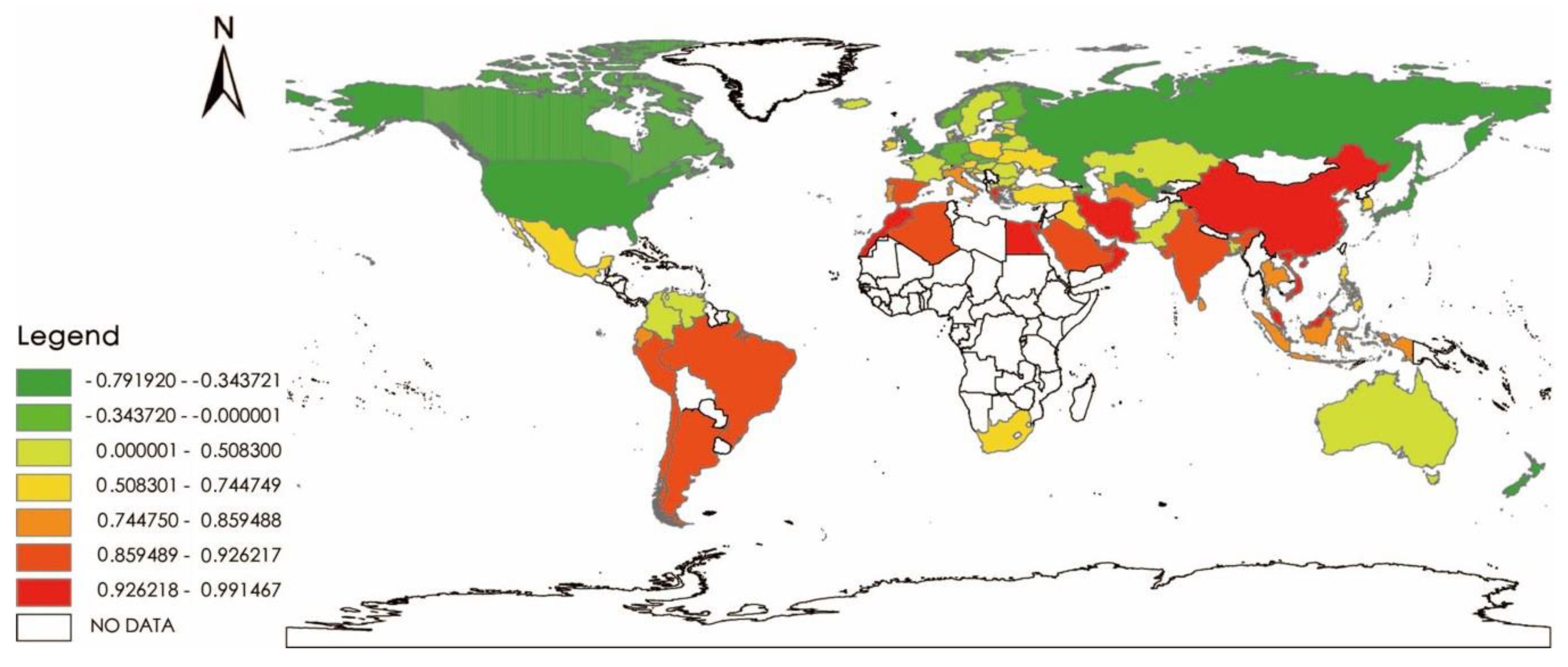
In the spatial dimension, the correlation between them also had spatial heterogeneity. In Southeast Asia, Africa, the Middle East, and South America, the relationship between them was positive. However, in North America and Europe, the relationship between them was negative. The correlation coefficients of developing countries were generally positive and high; China had the highest, at 0.9915. But developed countries were generally low or showed a negative correlation; Canada had the largest negative correlation, at −0.7919; Nordic countries were close to 0; and some European countries near Africa had higher correlation coefficients, such as Spain and Greece (

Table 3. Correlation coefficients of every country.

Country	Value	Group	Country	Value	Group	Country	Value	Group
China	0.9915 ***	1	Thailand	0.8035 ***	3	Romania	0.2108 *	5
Oman	0.9872 ***	1	Portugal	0.7689 ***	3	Belarus	0.2089 *	5
Morocco	0.9727 ***	1	Turkey	0.7447 ***	4	Bulgaria	0.1552 *	5
Egypt	0.9713 ***	1	Austria	0.7446 ***	4	Colombia	0.0855	5
Iran	0.9676 ***	1	South Africa	0.7339 ***	4	Sweden	0.0844	5
Qatar	0.9676 ***	1	Ireland	0.7324 ***	4	Hungary	0.0685	5
United Arab Emirates	0.9666 ***	1	Latvia	0.6990 ***	4	Luxembourg	0.0511	5
Vietnam	0.9599 ***	1	Kuwait	0.6969 ***	4	Denmark	0.0448	5
Malaysia	0.9549 ***	1	Ukraine	0.6908 ***	4	Norway	−0.0050	6
Cyprus	0.9439 ***	1	Croatia	0.6857 ***	4	Czech Republic	−0.0433	6
Greece	0.9402 ***	1	Iraq	0.6783 ***	4	Finland	−0.0636	6
Chile	0.9262 ***	2	Poland	0.6620 ***	4	Azerbaijan	−0.1328 *	6
Algeria	0.9229 ***	2	South Korea	0.6594 ***	4	Germany	−0.1357 *	6
Saudi Arabia	0.9206 ***	2	Mexico	0.6534 ***	4	Singapore	−0.1991 *	6
Argentina	0.9046 ***	2	Philippines	0.6467 ***	4	Slovakia	−0.2504 *	6
Trinidad & Tobago	0.9016 ***	2	France	0.5083 ***	5	Russian Federation	−0.3437 **	7
Spain	0.8933 ***	2	Kazakhstan	0.4710 **	5	Belgium	−0.3663 ***	7
India	0.8915 ***	2	Pakistan	0.4366 ***	5	New Zealand	−0.3758 **	7
Brazil	0.8905 ***	2	Venezuela	0.4212 ***	5	Netherlands	−0.4543 ***	7
Peru	0.8744 ***	2	Slovenia	0.3952 ***	5	Uzbekistan	−0.5882 **	7
Indonesia	0.8595 ***	3	Iceland	0.3653 ***	5	Lithuania	−0.6020 ***	7
Sri Lanka	0.8578 ***	3	Estonia	0.3219 **	5	United Kingdom	−0.6173 ***	7
Ecuador	0.8574 ***	3	Macedonia	0.3163 **	5	Japan	−0.6320 ***	7
Turkmenistan	0.8281 ***	3	Switzerland	0.2871 *	5	United States	−0.6602 ***	7
Israel	0.8139 ***	3	Australia	0.2566 **	5	Canada	−0.7919 ***	7
Italy	0.8125 ***	3	Bangladesh	0.2298 **	5

Note: * Denotes rejection of null hypothesis at 10% significance levels; ** Denotes rejection of null hypothesis at 5% significance levels; *** Denotes rejection of null hypothesis at 1% significance levels.

). Using to the spatial classification method [45], we divided the whole sample into seven groups. The results are shown in Figure 3.

The mean correlation coefficient of the whole sample was 0.4290; by analogy, Group 1 was 0.9658, Group 2 was 0.9028, Group 3 was 0.8252, Group 4 was 0.6945, Group 5 was 0.2589, Group 6 was −0.1186, and Group 7 was −0.5432 (

Table 4. Descriptive statistics of correlation results.

Statistics	All	Group 1	Group 2	Group 3	Group 4	Group 5	Group 6	Group 7
Number of samples	77	11	9	8	13	19	7	10
Mean	0.4290	0.9658	0.9028	0.8252	0.6945	0.2589	−0.1186	−0.5432
Max	0.9915	0.9915	0.9262	0.8595	0.7447	0.5083	−0.0050	−0.3437
Min	−0.7919	0.9402	0.8744	0.7689	0.6467	0.0448	−0.2504	−0.7919
Standard deviation	0.5148	0.0158	0.0175	0.0321	0.0349	0.1500	0.0875	0.1496
Coefficient of variation	1.2	0.0164	0.0194	0.0389	0.0503	0.5794	−0.7378	−0.2754

). The highest was China and the lowest was Canada. The standard deviations of groups with a larger mean were smaller, such as Groups 1 and 2; those with smaller means were larger, such as Groups 5 and 7.

4.2. Stationarity Test

Three methods (the HT, LLC, and ADF tests) were used in this study. If the cross-sectional dimension of panel data is large and the time dimension is small, it is called short panel, and vice versa. The whole sample group is short panel, which is tested by the HT and the ADF methods. From Group 1 to Group 7, all groups are long panel, which are tested by the LLC and the ADF methods. The results are shown in Table 5. Following the principle of majority, when the test results show that the series is stationarity many times, it means that the series is stationarity, and vice versa. In the nighttime light intensity series, the whole sample group, Group 4, Group 5, Group 6, and Group 7 were stationarity; Group 1, Group 2, and Group3 were non-stationarity. In the electric power consumption series, Group 3, Group 5, Group 6, and Group 7 were stationarity; the whole sample group, Group 1, Group 2, and Group 4 were non-stationarity.

Based on the stationarity test results, Groups 5, 6, and 7 could be used for the causality test. Groups 1 and 2 needed to use the cointegration test (

Table 6. Summary of stationarity tests.

Test Method		All	Group 1	Group 2	Group 3	Group 4	Group 5	Group 6	Group 7
Light	Fisher-ADF	yes	no	no	yes	yes	yes	yes	yes
	LLC or HT	yes	no	no	no	yes	yes	yes	yes
	Conclusion	yes	no	no	no	yes	yes	yes	yes
Electricity	Fisher-ADF	no	no	no	yes	no	yes	yes	yes
	LLC or HT	no	no	no	yes	yes	yes	yes	yes
	Conclusion	no	no	no	yes	no	yes	yes	yes
Next step		End	Cointegration test	Cointegration test	End	End	Causality test	Causality test	Causality test

). The test process for Group 3 and Group 4 did not go on to the next step, as there was no causal relationship between nighttime light intensity and electric power consumption in the whole sample group, Group 3, and Group 4.

4.3. Cointegration Test

In this study, we used three methods to test cointegration: The Kao test, the Pedroni test, and the Westerlund test. The results are shown in

Table 7. Panel cointegration test.

Test Method	Statistics	Group 1	Group 2
Kao test	Modified Dickey-Fuller t	−4.6383 ***	−2.6347 ***
	Dickey-Fuller t	−2.8722 ***	−2.3908 ***
	Augmented Dickey-Fuller t	−2.5286 ***	0.1048
	Unadjusted modified Dickey-Fuller t	−4.6378 ***	−3.2883 ***
	Unadjusted Dickey-Fuller t	−2.8721 ***	−2.6374 ***
Pedroni test	Modified Phillips-Perron t	−1.1674	1.0486
	Phillips-Perron t	−2.8284 ***	−0.3223
	Augmented Dickey-Fuller t	−1.9415 **	−0.4606
Westerlund test	Variance ratio	−3.0386 ***	−0.3142

Note: * Denotes rejection of null hypothesis at 10% significance levels; ** Denotes rejection of null hypothesis at 5% significance levels; *** Denotes rejection of null hypothesis at 1% significance levels.

. By comparing three panel data cointegration test results, there was a cointegration relationship between nighttime light intensity and electric power consumption levels in Group 1 and Group 2. So, two groups could be used for panel data causal analysis in the next step.

4.4. Causality Test

For the whole sample, Group 3, and Group 4, a panel Granger causality test could not be performed, because they did not meet the basic conditions of the causality test. Therefore, we could not judge whether there was Granger homogeneous causality in these groups. Based on results of Group 2 and Group 7, electric power consumption was the Granger cause of light intensity. But nighttime light intensity was not the Granger cause of electric power consumption. For Groups 1, 5, and 6, electric power consumption was the Granger cause of nighttime light intensity, and nighttime light intensity was also the Granger cause of electric power consumption (

Table 8. Panel causality test.

Original Hypothesis	Light does not Homogeneously Cause EC		EC does not Homogeneously Cause Light
	Number of Lags	Z-Bar Statistics	Number of Lags	Z-Bar Statistics
All	-	-	-	-
Group 1	5	2.3734 **	5	7.8490 ***
Group 2	5	0.5494	1	8.7235 ***
Group 3	-	-	-	-
Group 4	-	-	-	-
Group 5	5	7.9996 ***	5	12.1145 ***
Group 6	5	3.4454 ***	5	21.2654 ***
Group 7	5	1.1762	5	10.6500 ***

Note: * Denotes rejection of null hypothesis at 10% significance levels; ** Denotes rejection of null hypothesis at 5% significance levels; *** Denotes rejection of null hypothesis at 1% significance levels.

).

5. Discussion

According to the correlation results, there was spatial heterogeneity between power consumption and nighttime light data. Developing countries, such as China and Vietnam, generally had a high and positive correlation; developed countries generally had a low or even negative correlation. According to the causal analysis, there was no causal relationship in the world as a whole, but there was local causality. In developing countries and regions with a strong correlation, such as Asia, South America, and Africa, the results showed that there was causality between power consumption and nighttime light intensity; in developed countries, there was no causality between power consumption and nighttime light intensity. The reasons are mainly the following:

• First, the impact of a country’s electric power consumption structure on the estimation results; the electricity structure of developed countries is more complex, and the electricity structure of developing countries is simple.
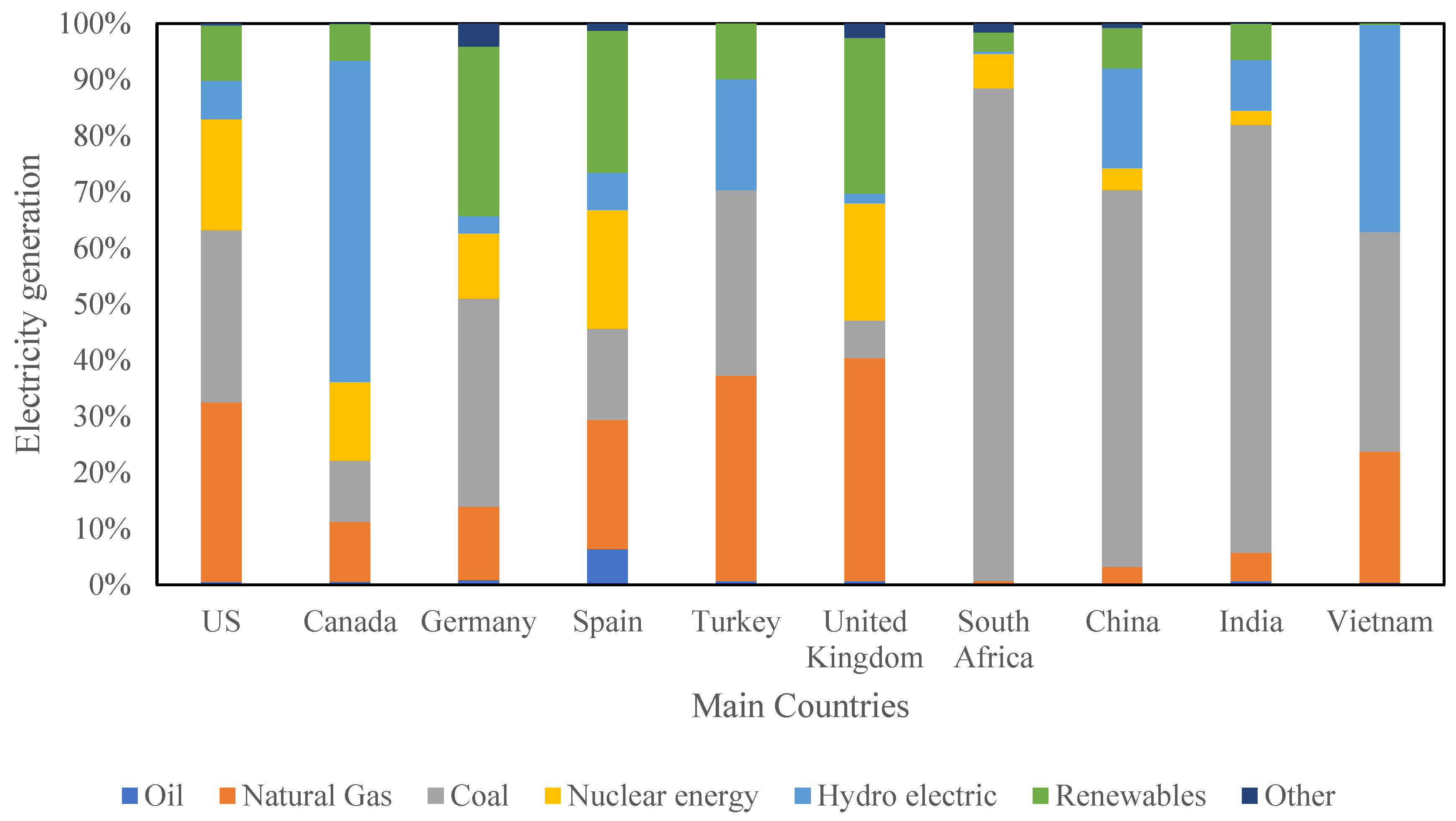
• Second, the power supply structure of developed countries also has a greater impact; the power supply channels of developed countries are diversified and the proportion of renewable energy is higher, such as in the Nordic region, while developing countries generally still use hydroelectric or coal-fired power generation (Figure 4).
• Third, there is a spatial spillover effect of nighttime light, near Africa and the Middle East; some European countries have strong positive correlation, such as Portugal, Spain, Turkey, and Ireland, while other European countries have weak or negative correlation (Figure 3).

In general, we can draw some conclusions. First, nighttime light data can be used to estimate power consumption intensity in some areas. The estimates of developing countries regions, such as Southeast Asia and the Middle East, are more accurate. Using nighttime light data to directly estimate the economic and social indicators of developed countries has a large error. Second, in the contiguous regions between Africa, the Middle East, and Europe, such as Spain and Turkey, the nighttime light spillover effect is relatively strong, which is not suitable for estimating socioeconomic indicators. Third, for developed countries, it is necessary to introduce more variables, such as urban population, spatial climate conditions, and so on, to estimate economic and social indicators using nighttime light data.

6. Conclusions

In order to evaluate the applicability of nighttime light data in estimating socioeconomic indicators, we propose a causal-effect inference method to test the relationship between nighttime light data and socioeconomic indicators. According to the method, we found evidence to support applications of nighttime light data in the estimation of socioeconomic indicators. At the same time, we find that some conclusions are of great significance to the application of light data. The main conclusions are as follows:

• Casual inference is necessary before estimating socioeconomic indicators by nighttime light data.
• Spatial heterogeneity exists in the applicability of nighttime light data in estimating socioeconomic indicators.
• Nighttime light data are more suitable for estimating electric power consumption in developing countries, such as China, India, and so on.
• For developed countries, it is necessary to add more latent variables, such as urban population, spatial climate conditions, and so on, to estimate electric power consumption using nighttime light data.
• In the contiguous regions of geography, such as regions between Africa, the Middle East, and Europe, the nighttime light spillover effect is relatively strong. So, nighttime light data need to be corrected.

Nighttime light data are publicly accessible data in practice. In academic research and practice, economists, geographers, and ecologists regard it as an important tool and are widely used. Through this study, we should pay more attention to correlative and causal relationships in future practice. The correlation between nighttime light data and economic and social indicators is not equal to causality. When using nighttime light data in practice, theoretical causal inference is a necessary process. And, the method proposed in this paper can be used to test other research objects, such as metal stocks, population, GDP, etc. And this method is also applicable when the statistical data of smaller spatial units, such as the province level, the city level, or smaller units, can be obtained. Future research should pay more attention to the intrinsic logical relationship between nighttime light data and socioeconomic indicators. In future research, the relationship between nighttime light and socioeconomic indicators on the spatial dimension is important in this field. In order to estimate the socioeconomic indicators more accurately using light data, it is necessary to deal with the spatial dependence of nighttime light data.

References

- Li, H.M.; Zhao, X.F.; Wu, T.; Qi, Y. The consistency of China’s energy statistics and its implications for climate policy. J. Clean. Prod. 2018, 199, 27–35. [Google Scholar] [CrossRef]
- Croft, T.A. Nighttime images of the earth from space. Sci. Am. 1978, 239, 86–101. [Google Scholar] [CrossRef]
- Elvidge, C.D.; Hsu, F.-C.; Baugh, K.E.; Ghosh, T. National trends in satellite-observed lighting. Glob. Urban Monit. Assess. Earth Obs. 2014, 23, 97–118. [Google Scholar]
- Elvidge, C.D.; Baugh, K.E.; Kihn, E.A.; Kroehl, H.W.; Davis, E.R.; Davis, C.W. Relation between satellite observed visible-near infrared emissions, population, economic activity and electric power consumption. Int. J. Remote Sens. 1997, 18, 1373–1379. [Google Scholar] [CrossRef]
- Lo, C.P. Urban indicators of China from radiance-calibrated digital DMSP-OLS nighttime images. Ann. Assoc. Am. Geogr. 2002, 92, 225–240. [Google Scholar] [CrossRef]
- Zhou, Y.Y.; Smith, S.J.; Zhao, K.G.; Imhoff, M.; Thomson, A.; Bond-Lamberty, B.; Asrar, G.; Zhang, X.S.; He, C.Y.; Elvidge, C.D. A global map of urban extent from nightlights. Environ. Res. Lett. 2015, 10. [Google Scholar] [CrossRef]
- Gallaway, T.; Olsen, R.N.; Mitchell, D.M. The economics of global light pollution. Ecol. Econ. 2010, 69, 658–665. [Google Scholar] [CrossRef]
- Shi, K.F.; Yu, B.L.; Huang, Y.X.; Hu, Y.J.; Yin, B.; Chen, Z.Q.; Chen, L.J.; Wu, J.P. Evaluating the Ability of NPP-VIIRS Nighttime Light Data to Estimate the Gross Domestic Product and the Electric Power Consumption of China at Multiple Scales: A Comparison with DMSP-OLS Data. Remote Sens. 2014, 6, 1705–1724. [Google Scholar] [CrossRef] [Green Version]
- Henderson, J.V.; Storeygard, A.; Weil, D.N. Measuring Economic Growth from Outer Space. Am. Econ. Rev. 2012, 102, 994–1028. [Google Scholar] [CrossRef]
- Zhang, Q.L.; Seto, K.C. Mapping urbanization dynamics at regional and global scales using multi-temporal DMSP/OLS nighttime light data. Remote Sens. Environ. 2011, 115, 2320–2329. [Google Scholar] [CrossRef]
- Ma, T.; Zhou, C.H.; Pei, T.; Haynie, S.; Fan, J.F. Quantitative estimation of urbanization dynamics using time series of DMSP/OLS nighttime light data: A comparative case study from China’s cities. Remote Sens. Environ. 2012, 124, 99–107. [Google Scholar] [CrossRef]
- Elvidge, C.D.; Ziskin, D.; Baugh, K.E.; Tuttle, B.T.; Ghosh, T.; Pack, D.W.; Erwin, E.H.; Zhizhin, M. A Fifteen Year Record of Global Natural Gas Flaring Derived from Satellite Data. Energies 2009, 2, 595–622. [Google Scholar] [CrossRef]
- Do, Q.T.; Shapiro, J.N.; Elvidge, C.D.; Abdel-Jelil, M.; Ahn, D.P.; Baugh, K.; Hansen-Lewis, J.; Zhizhin, M.; Bazilian, M.D. Terrorism, geopolitics, and oil security: Using remote sensing to estimate oil production of the Islamic State. Energy Res. Soc. Sci. 2018, 44, 411–418. [Google Scholar] [CrossRef] [PubMed] [Green Version]
- Xiao, H.; Ma, Z.; Mi, Z.; Kelsey, J.; Zheng, J.; Yin, W.; Yan, M. Spatio-temporal simulation of energy consumption in China’s provinces based on satellite night-time light data. Appl. Energy 2018, 231, 1070–1078. [Google Scholar] [CrossRef]
- Tripathy, B.R.; Sajjad, H.; Elvidge, C.D.; Ting, Y.; Pandey, P.C.; Rani, M.; Kumar, P. Modeling of Electric Demand for Sustainable Energy and Management in India Using Spatio-Temporal DMSP-OLS Night-Time Data. Environ. Manag. 2018, 61, 615–623. [Google Scholar] [CrossRef] [PubMed]
- Shi, K.F.; Yu, B.L.; Huang, C.; Wu, J.P.; Sun, X.F. Exploring spatiotemporal patterns of electric power consumption in countries along the Belt and Road. Energy 2018, 150, 847–859. [Google Scholar] [CrossRef]
- Tyralis, H.; Mamassis, N.; Photis, Y.N. Spatial analysis of the electrical energy demand in Greece. Energy Policy 2017, 102, 340–352. [Google Scholar] [CrossRef]
- Xie, Y.H.; Weng, Q.H. World energy consumption pattern as revealed by DMSP-OLS nighttime light imagery. Gisci. Remote Sens. 2016, 53, 265–282. [Google Scholar] [CrossRef]
- Xie, Y.H.; Weng, Q.H. Detecting urban-scale dynamics of electricity consumption at Chinese cities using time-series DMSP-OLS (Defense Meteorological Satellite Program-Operational Linescan System) nighttime light imageries. Energy 2016, 100, 177–189. [Google Scholar] [CrossRef]
- Shi, K.F.; Chen, Y.; Yu, B.L.; Xu, T.B.; Yang, C.S.; Li, L.Y.; Huang, C.; Chen, Z.Q.; Liu, R.; Wu, J.P. Detecting spatiotemporal dynamics of global electric power consumption using DMSP-OLS nighttime stable light data. Appl. Energy 2016, 184, 450–463. [Google Scholar] [CrossRef]
- Letu, H.; Hara, M.; Yagi, H.; Tana, G.; Nishio, F. Estimating the energy consumption with nighttime city light from the DMSP/OLS imagery. In Proceedings of the 2009 Joint Urban Remote Sensing Event, Shanghai, China, 20–22 May 2009. [Google Scholar]
- He, C.Y.; Ma, Q.; Li, T.; Yang, Y.; Liu, Z.F. Spatiotemporal dynamics of electric power consumption in Chinese Mainland from 1995 to 2008 modeled using DMSP/OLS stable nighttime lights data. J. Geogr. Sci. 2012, 22, 125–136. [Google Scholar] [CrossRef]
- Shi, K.F.; Chen, Y.; Li, L.Y.; Huang, C. Spatiotemporal variations of urban CO2 emissions in China: A multiscale perspective. Appl. Energy 2018, 211, 218–229. [Google Scholar] [CrossRef]
- Wang, S.J.; Liu, X.P. China’s city-level energy-related CO2 emissions: Spatiotemporal patterns and driving forces. Appl. Energy 2017, 200, 204–214. [Google Scholar] [CrossRef]
- Shi, K.F.; Chen, Y.; Yu, B.L.; Xu, T.B.; Chen, Z.Q.; Liu, R.; Li, L.Y.; Wu, J.P. Modeling spatiotemporal CO2 (carbon dioxide) emission dynamics in China from DMSP-OLS nighttime stable light data using panel data analysis. Appl. Energy 2016, 168, 523–533. [Google Scholar] [CrossRef]
- Ghosh, T.; Elvidge, C.D.; Sutton, P.C.; Baugh, K.E.; Ziskin, D.; Tuttle, B.T. Creating a Global Grid of Distributed Fossil Fuel CO2 Emissions from Nighttime Satellite Imagery. Energies 2010, 3, 1895–1913. [Google Scholar] [CrossRef]
- Meng, L.N.; Graus, W.; Worrell, E.; Huang, B. Estimating CO2 (carbon dioxide) emissions at urban scales by DMSP/OLS (Defense Meteorological Satellite Program’s Operational Linescan System) nighttime light imagery: Methodological challenges and a case study for China. Energy 2014, 71, 468–478. [Google Scholar] [CrossRef]
- Liang, H.W.; Dong, L.; Tanikawa, H.; Zhang, N.; Gao, Z.Q.; Luo, X. Feasibility of a new-generation nighttime light data for estimating in-use steel stock of buildings and civil engineering infrastructures. Resour. Conserv. Recy. 2017, 123, 11–23. [Google Scholar] [CrossRef]
- Liang, H.W.; Tanikawa, H.; Matsuno, Y.; Dong, L. Modeling In-Use Steel Stock in China’s Buildings and Civil Engineering Infrastructure Using Time-Series of DMSP/OLS Nighttime Lights. Remote Sens. 2014, 6, 4780–4800. [Google Scholar] [CrossRef]
- Hattori, R.; Horie, S.; Hsu, F.C.; Elvidge, C.D.; Matsuno, Y. Estimation of in-use steel stock for civil engineering and building using nighttime light images. Resour. Conserv. Recy. 2014, 83, 229–233. [Google Scholar] [CrossRef]
- Taguchi, G.; Hsu, F.C.; Tanikawa, H.; Matsuno, Y. Estimation of Steel Use in Buildings by Night Time Light Image and GIS. Tetsu Hagane 2012, 98, 450–456. [Google Scholar] [CrossRef] [Green Version]
- Takahashi, K.I.; Terakado, R.; Nakamura, J.; Adachi, Y.; Elvidge, C.D.; Matsuno, Y. In-use stock analysis using satellite nighttime light observation data. Resour. Conserv. Recy. 2010, 55, 196–200. [Google Scholar] [CrossRef]
- Takahashi, K.I.; Terakado, R.; Nakamura, J.; Daigo, I.; Matsuno, Y.; Adachi, Y. In-Use Stock of Copper Analysis Using Satellite Nighttime Light Observation Data. Mater. Trans. 2009, 50, 1871–1874. [Google Scholar] [CrossRef] [Green Version]
- Ji, G.X.; Tian, L.; Zhao, J.C.; Yue, Y.L.; Wang, Z. Detecting spatiotemporal dynamics of PM2.5 emission data in China using DMSP-OLS nighttime stable light data. J. Clean. Prod. 2019, 209, 363–370. [Google Scholar] [CrossRef]
- Amaral, S.; Câmara, G.; Monteiro, A.M.V.; Quintanilha, J.A.; Elvidge, C.D. Estimating population and energy consumption in Brazilian Amazonia using DMSP night-time satellite data. Comput. Environ. Urban Syst. 2005, 29, 179–195. [Google Scholar] [CrossRef]
- BP. Statistical Review of World Energy 2018; BP: London, UK, 2018. [Google Scholar]
- Choi, I. Unit root tests for panel data. J. Int. Money Financ. 2001, 20, 249–272. [Google Scholar] [CrossRef]
- Im, K.S.; Pesaran, M.H.; Shin, Y. Testing for unit roots in heterogeneous panels. J. Econom. 2003, 115, 53–74. [Google Scholar] [CrossRef]
- Levin, A.; Lin, C.F.; Chu, C.S.J. Unit root tests in panel data: Asymptotic and finite-sample properties. J. Econom. 2002, 108, 1–24. [Google Scholar] [CrossRef]
- Pedroni, P. Critical values for cointegration tests in heterogeneous panels with multiple regressors. Oxf. B Econ. Stat. 1999, 61, 653–670. [Google Scholar] [CrossRef]
- Newey, W.K.; West, K.D. Automatic Lag Selection in Covariance-Matrix Estimation. Rev. Econ. Stud. 1994, 61, 631–653. [Google Scholar] [CrossRef]
- Lopez, L.; Weber, S. Testing for Granger causality in panel data. Stata J. 2017, 17, 972–984. [Google Scholar] [CrossRef]
- Dumitrescu, E.I.; Hurlin, C. Testing for Granger non-causality in heterogeneous panels. Econ. Model. 2012, 29, 1450–1460. [Google Scholar] [CrossRef] [Green Version]
- Granger, C.W.J. Investigating Causal Relations by Econometric Models and Cross-Spectral Methods. Econometrica 1969, 37, 424–438. [Google Scholar] [CrossRef]
- Anselin, L. Thirty years of spatial econometrics. Pap. Reg. Sci. 2010, 89, 3–25. [Google Scholar] [CrossRef]
- Gollini, I.; Lu, B.; Charlton, M.; Brunsdon, C.; Harris, P. GWmodel: An R package for exploring spatial heterogeneity using geographically weighted models. arXiv 2013, arXiv:1306.0413 2013. [Google Scholar] [CrossRef]
- Jenks, G.F. The data model concept in statistical mapping. Int. Yearb. Cartogr. 1967, 7, 186–190. [Google Scholar]
- Breitung, J. The local power of some unit root tests for panel data. Adv. Econom. 2000, 15, 161–177. [Google Scholar]
- Maddala, G.S.; Wu, S.W. A comparative study of unit root tests with panel data and a new simple test. Oxf. B Econ. Stat. 1999, 61, 631–652. [Google Scholar] [CrossRef]
- Granger, C.W.J. Testing for Causality—A Personal Viewpoint. J. Econ. Dyn. Control 1980, 2, 329–352. [Google Scholar] [CrossRef]
Figure 1.
Analysis flow chart.
Figure 2.
Correlation coefficients over time. Note: Correlation coefficients were calculated by 77 countries every year.
Figure 3.
Correlation coefficients in the spatial dimension.
Figure 4.
Electric power generation structure in major countries.