AUD-MTS: An Abnormal User Detection Approach Based on Power Load Multi-Step Clustering with Multiple Time Scales


State Key Lab of Networking and Switching Technology, Beijing University of Posts and Telecommunications, Beijing 100876, China
*
Authors to whom correspondence should be addressed.
Energies 2019, 12(16), 3144; https://doi.org/10.3390/en12163144
Submission received: 18 July 2019
/
Revised: 8 August 2019
/
Accepted: 12 August 2019
/
Published: 15 August 2019
(This article belongs to the Section A1: Smart Grids and Microgrids)
Abstract
:With the rapid growth of Smart Grid, electricity load analysis has become the simplest and most effective way to divide user groups and understand user behavior. This paper proposes an AUD-MTS (Abnormal User Detection approach based on power load multi-step clustering with Multiple Time Scales). Firstly, we combine RBM (Restricted Boltzmann Machine) hidden feature learning with K-Means clustering to extract typical load patterns in the short-term. Secondly, time scale conversion is performed so that the analysis subject can be transformed from load pattern to user behavior. Finally, a two-step clustering in long-term is adopted to divide users from both coarse-grained and fine-grained dimensions so as to detect abnormal users referring to customized OutlierIndex. Experiments are conducted using annual 24-point power load data of American users in all states. The accuracy of clustering methods in AUD-MTS reaches 87.5% referring to the 16 commercial building types defined by the U.S. Department of Energy, which outperforms other common clustering algorithms on AMI (Advanced Metering Infrastructure). After that, the OutlierIndex score of AUD-MTS can be increased by 0.16 compared with other outlier detection algorithms, which shows that the proposed method can detect abnormal users precisely and efficiently. Furthermore, we summarized possible causes including federal holidays, climate zones and summertime that may lead to abnormal behavior changes and discussed countermeasures respectively, which accounts for 82.3% of anomalies. The rest may be potential electricity stealing users, which requires further investigation.
1. Motivation
Driven by the awareness of green energy conservation, countries are vigorously developing smart grids, which are the product of the coordinated development of existing technologies and new technologies, such as networks and smart meters. What is more, it ensures a two-way interaction between the grids and consumers. The annual growth rate of 18.2% of the global smart grid market since 2013 suggests smart grids to be the key to changing future energy system scenarios [1]. Therefore, much research has been conducted, including power load analysis and abnormal user detection [2]. The trend of getting multi-source, heterogeneous and massive data, and how to discover typical load patterns and divide various customers using original load data has become the current hotspot of power industry. However, common load pattern analysis usually depends on single-day or full-year power load data, which lacks the connection and expansion in the time dimension. Moreover, the current user profile is usually carried out by clustering according to artificial indexes, with abnormal user detection implemented manually. How to analyze load data on multiple time scales, extract typical load patterns and automatically filter outliers will become the next focused field.
Load pattern analysis means extracting typical load patterns from original data through data processing and clustering. This is the simplest and most effective way to analyze power load, in which lots of research work has been carried out. In terms of modeling and clustering, Chicco [3] provided an overview of the suitable clustering techniques to group customers, along with analyzing power load pattern data. A series of profile classes reflective of home electricity use were constructed by McLoughlin et al. [4], and Panapakidis et al. [5] proposed a comprehensive methodology, which uses clustering techniques to investigate the electricity behavior of buildings. Modeling and validation of electrical load profiling in residential buildings in Singapore were introduced by Luo [6] and a method based on one-year field measurement to develop a load characteristic curve based on static load model in medium voltage distribution network is designed [7]. Li et al. [8] proposed a smart data-analysis method with outlier detection, to predict daily electricity consumption in buildings. A mixed model was built to group similar load profiles by Labeeuw et al. [9] while Mets et al. [10] chose a two-stage load pattern clustering. As for algorithm details, Chicco et al. [11] used support vector clustering (SVC) with Gaussian kernel for electrical load pattern classification and illustrated an original Electrical Pattern Ant Colony Clustering (EPACC) algorithm in 2013 [12]. Also, Zhang et al. [13] determined the most suitable clustering algorithm and the priority rank of clusters by a stability index and a priority index, respectively.
Normally, the users’ electricity consumption behavior is regular and controllable, but abnormal consumption behavior will bring unexpected losses to the power supply side, such as power stealing behavior, etc. On one hand, abnormal user detection can help companies identify outliers with unusual behaviors, analyze their behavior changes and then improve service strategies. As a practice, an algorithm, based on probabilistic data mining and time series analysis, was introduced for detecting consumption outliers in smart grids [14]. Capozzoli et al. [15] proposed an automatic load pattern learning and anomaly detection method to improve energy management in intelligent buildings. Seem [16] proposed a novel method for the identification of abnormal energy consumption in buildings, which relied on the analysis of daily energy consumption and peak energy consumption. Tang et al. [17] analyzed the periodic patterns in the data and reorganizes the data for ease of analysis. In other energy fields, a hybrid forecasting model was designed and used in Hainan wind farm of China, which also relied on detecting outlier [18].
On the other hand, user behavior clustering is the foundation of understanding customer motivation, forming specific customer clusters which have similar patterns and providing different clusters customized services. For example, Chicco et al. [19] compared the results obtained by using various unsupervised clustering algorithms for electricity customer classification. Within all these algorithms, Chicco et al. [20] focused on classifying customers by applying a modified follow-the-leader algorithm with the self-organizing maps and used the indices as distinctive features to divide customers into classed [21]. Viegas et al. [22] studied the new residential electricity classification by combing smart metering, survey data and model-based feature selection while Quilumba et al. [23] predicted load by identifying groups of customers after clustering with similar load consumption patterns. Besides, Teeraratkul et al. [24] proposed a shape-based approach that predicted household consumer energy consumption behaviors with better classification. What is more, a method for identifying and improving the household behavior in residential buildings was developed [25] and daily electricity consumption profiles from smart meters were regarded as an active behavior agent for space heating and cooling [26].
Analysis with multiple time scales means analyzing data from different time dimensions, with the aim of discovering different trends in both short-term and long-term. More particularly, multi-timescale analysis is quite suitable for time-series data and has been applied in various fields. Such as in energy fields in distinct building environment, supervised machine learning models for predicting energy in the short, medium and long-term were introduced [27]. Ahmad et al. [28] analyzed the potential of three variant machine-learning models on predicting district level energy demand in the medium and long-term in smart grids, respectively. Huang et al. [29] examined impacts of oil supply and demand, the world economy and the political stability on oil price fluctuations in multiple time horizons. Pan et al. [30] studied the interactions in a district electricity and heating systems considering the time-scale characteristics. Besides, an optimization method was used in the design of a bottom-fixed OWC (Oscillating Water Column), which focused on the importance of time scales [31]. Bhattarai et al. [32] presented a multi-timescale control strategy for deploying electric vehicles (EV). In electricity storage, a combined assessment methodology was proposed to compare the stationary electricity storage technologies of different time and system scales [33]. In electronics field, an islanded medium-voltage (MV) microgrid placed in Dongao Island was presented with dynamic stability control from different time scales [34]. As for dispatching systems, a two-time-scale decision strategy has been developed to provide provable power costs and delay guarantees in distributed data centers [35].
In summary, there has been lots of research work in load pattern clustering and abnormal user detection while analysis with multiple time scales is applied in various fields. However, little attention was paid to combining these three aspects together. In this paper, an abnormal user detection approach based on power load multi-step clustering with multiple time scales (AUD-MTS) was proposed. In this paper we use Restricted Boltzmann Machine (RBM) to learn hidden features so as to extract typical load patterns in short-term. Meanwhile, we divide all the customers and analyze their behavior changes in long-term by transforming data dimensions. Finally, abnormal user detection is implemented with the help of customized Outlier Index.
Compared to other common methods, this scheme can learn abstract period characteristics automatically and analyze electricity consumption behaviors in both short-term and long-term, which leads to a more accurate abnormal user detection and user classification. With all detected abnormal users, we can discuss countermeasures respectively referring to different causes so as to avoid excessive power load. Further research could be done to check whether there is an electricity stealing behavior or not for each abnormal user.
In this paper, we introduce the methodology of proposed AUD-MTS in Section 2, including the overall process and the algorithm steps. Experiments on both load pattern clustering in short-term and two-step user clustering in long-term have been conducted in Section 3. What is more, we detect abnormal users from each cluster and analyze the possible influencing factors, along with doing some comparison with other common outlier detection algorithms in Section 4. Finally, in Section 5, we conclude this paper.
2. Methodology of AUD-MTS
Problem definition: Since user load data is collected, we need to find representative characteristics first such as period, peak-valley difference and other hidden features. How to classify load patterns according to these characteristics in short-term is the first difficulty. Secondly, we need to convert time scales so as to transform the analysis subject from load pattern to user behavior, where how to build user behavior model is the next problem. Furthermore, a precise division of users in long-term is required in order to analyze typical user behaviors. Finally, we need to filter abnormal users from each cluster and explore the reasons for unusual behavior changes, which is the main purpose of the whole method.
Data definition: The data input is 24-point electricity data from n users, which is collected during a whole year and forms the annual electricity load data set . The annual load data consists of 52 weeks, which can be divided into weekly load data set . where each unit is a vector with 168 data points . Among them, weekly load data is used for load pattern analysis in short-term while annual load data is for user analysis in long-term with the help of short-term clustering results.
In short time scale analysis, we use RBM model to solve network variables so as to obtain hidden features that are difficult to find manually. During this process, the training input is 168-dimensional weekly load vector and the output is m-dimensional hidden features . The short-time scale analysis will perform a series of preprocessing and clustering analysis based on these m-dimensional hidden features.
2.1. Overall Process
As Figure 1 shows above, it can be seen that AUD-MTS approach consists of four stages: load pattern clustering in short-term, time scale conversion, user clustering in long-term and outlier detection. Short-term load clustering divides weekly load patterns by learning hidden features through RBM model from a short time scale. Time scale conversion connects weekly clustering to annual analysis so that the analysis subject can be converted into user electricity behavior model, which prepares for the next user analysis and abnormal user detection. Based on the user model, long-term user clustering realizes the division of electricity users from different grain levels. As the ultimate goal, outlier detection screens abnormal users from each cluster and analyzes the possible influencing factors.
The whole process only needs to input 24-point electricity load data of all users and outputs abnormal user clusters, typical load patterns and user behavior classification through progressive analysis from short-term to long-term scale.
2.2. Algorithm Steps
2.2.1. Load Pattern Clustering in Short-Term
Short-term load pattern clustering mainly involves two processes of RBM feature learning and distance-based clustering, where the input is users’ 7-day power load data and typical weekly load patterns are calculated. Load data is first preprocessed to fill the vacancies and a maximum-minimum normalization operation is performed in order to avoid numerical influence. Then the Restricted Boltzmann Machine (RBM) model is trained to build hidden layer and learn hidden features. After the iteration converges or reaches the predetermined iteration round, the current output is the encoded hidden features, which is a more powerful and precise expression of the input data. In the end, K-Means clustering method is used to classify hidden features to obtain typical weekly load patterns, which means power load analysis on a short time scale is completed.
Restricted Boltzmann Machine (RBM) is an unsupervised neural network model, which is widely applied in dimensionality reduction, autoencoder and recommendation system. As the given network structure in Figure 2, RBM model consists of two layers of visible layer and hidden layer, corresponding to the 168-dimensional original load input and m-dimensional hidden features respectively.
RBM is an energy model, which the main idea is to train model by minimizing the overall energy of whole network. The RBM neural network will select an appropriate energy function, obtain the probability distribution of variables based on this energy function and then solve the maximum likelihood estimate based on the probability distribution:
RBM selects the energy model and solves the maximum of where and represent the state vector of visible layer and hidden layer respectively, and is composed of all training samples.
Here we use RBM to analyze power load in order to not only preserve the original data information, but also to find the period and trend features that are difficult to find manually. Throughout the training process, 168-dimensional weekly load data is input and m-dimensional hidden features are output, where a K-Means clustering will be performed based on calculated hidden features. After obtaining the classification of all categories, the trained RBM network will be reversely called so as to reconstruct weekly power consumption curves from hidden features of each cluster center and get typical load patterns in short-term eventually.
2.2.2. Time Scale Conversion
The phase of time scale conversion is intended to associate the weekly short-term load pattern clustering with the annual long-term user behavior analysis so that abnormal user detection task can be accomplished step by step. The conversion of the data model is shown as Figure 3.
- After clustering in short-term, the consumption curves have been reconstructed by hidden features of each cluster center with several typical load patterns obtained. In order to measure the differences among all clusters, a load pattern similarity matrix will be calculated based on the Euclidean distance.
- According to the short-term clustering result, annual 24-point load data T will be labelled to construct a user consumption behavior model, resulting in a long-term behavior vector L of 52 data points generated for each user.
- Taking both short-term load pattern similarity matrix and long-term behavior label L into consideration, the annual data of all users will be compared in pairs so that a user behavior similarity matrix D will be generated for the next analysis in long-term.
That is to say, in the conversion from short-term to long-term, the results of short-term clustering are taken as the input of the user behavior model. More specifically, every user behavior label corresponds to the clustering category of that particular week. As the time scale conversion Figure 4 shown above, the left side is the clustering result in short-term where the time scale is 168 h in a week while the right side is the generated user behavior model in long-term, where the time scale is 52 weeks in a year.
2.2.3. User Behavior Analysis in Long-Term
With the aim of detecting abnormal users and analyzing typical user consumption behaviors in long-term, this stage mainly involves a two-step clustering operation as the algorithm flowchart shown as Figure 5.
Since the user behavior similarity matrix D has been calculated, user behavior data is firstly clustered by Hierarchical Clustering according to the matrix, which leads to a coarse-grained user division. Then, the improved DBSCAN (Density-Based Spatial Clustering of Applications with Noise) clustering based on outliers is performed on each subclass to get a fine-grained division of users with abnormal users detected. This process needs to define Outlier Index which can improve accuracy and play a role in evaluation target so as to optimize the clustering parameters through grid search automatically. At last, we group all the abnormal users trying to analyze possible reasons that result in unusual behavior changes, which means user profile on multiple time scales is done completely.
Commonly used indicators for measuring clustering results such as Silhouette Coefficient, Rand index and Mutual Information only consider intra-cluster and inter-cluster distance, which cannot measure the impact of abnormal outliers on clustering results. More seriously, in a scenario where a coarse-grained clustering is reclassified, the indicators mentioned above may become invalid when the clustering result has only one category. To solve these problems, this paper defines OutlierIndex as follows:
OutlierIndex is calculated by using the average intra-cluster distance () and the average inter-cluster distance () for each cluster, with the minimum distance between abnormal samples and others ). To clarify, measures the distance between a sample and the nearest outlier. Note that the Outlier Index will get its maximum or minimum value when the clustering result has only one category. More specifically, the Infinity will be returned to terminate the iteration when all samples in this category are completely identical; Otherwise, if there is a gap among samples, it will be considered that the result can be further improved by re-clustering or applying outlier detection and a minimum of −1 will be returned. Values near 0 usually indicate overlapping clusters, while a higher score implies a better division.
The pseudo code of the whole algorithm is displayed as Figure 6, where the input is the user behavior similarity matrix, the output is screened abnormal users and a typical user classification. The main cycle is to optimize OutlierIndex with iterations. By using the OutlierIndex to guide two-step clustering, automatic abnormal user detection and user division process will be carried out.
3. Experiments
3.1. Data Preparation and Indicator Definition
In order to verify the accuracy of the algorithm for load pattern clustering and abnormal user detection, consumers’ annual 24-point load data are collected for the experiment of which geographic covers all states of the U.S. including Alaska and Hawaii. For the sake of making data distribution obey the population of states, we sample the data and choose 800 users eventually. User data has original labels which are 16-class commercial reference buildings classified by the U.S. Department of Energy according to its function and scale. Since the same label does not refer to the same load consumption habits, thus, it will be used as a reference for verification without joining in any process for training.
The U.S. Department of Energy (DOE) and three of its national laboratories developed commercial reference buildings. These 16 building types, representing approximately 70% of the commercial buildings in the U.S, cross all U.S. climate zones. All types include Large Office, Medium Office, Small Office, Warehouse, Stand-alone Retail, Strip Mall, Primary School, Secondary School, Supermarket, Quick Service Restaurant, Full Service Restaurant, Hospital, Outpatient Health Care, Small Hotel, Large Hotel and Midrise Apartment.
Examples of typical weekly and annual data curve are shown below as Figure 7. After collecting data, preprocess is first carried out. For vacancy and zero-value data, the mean value of adjacent data is padded. In order to avoid the influence of the absolute value of power consumption, the maximum-minimum normalization of the load data is performed. Then, the experiment data is reconstructed so as to detect abnormal users and analyze behaviors on different time scales. Each user’s annual power load data consists of 52 weeks, resulting in a total of 41,600 weekly load data reconstructed where each one contains 168 data points. In this paper, weekly load data is used for short-term load pattern clustering and user data is used for long-term outlier detection and user division.
In order to verify that the two-step clustering method can divide user groups precisely, we will compare it with other common clustering algorithms. Except for the OutlierIndex defined above, we will also select V_measure, Adjusted Mutual Information and Adjusted Rand Index as references during the comparison.
As defined above, the V_measure is the harmonic mean between homogeneity and completeness: A clustering result satisfies homogeneity if all of its clusters only contain data points which are members of a single class while a clustering result satisfies completeness if all the data points that are members of a given class are elements of the same cluster.
The Mutual Information (MI) is a measure of the similarity between two labels of the same data. Where is the number of the samples in cluster and the same to , the Mutual Information between clusters and V is given as:
Adjusted Mutual Information (AMI) is an adjustment for Mutual Information score with taking into account the chance as shown above.
Similarly, the Rand Index calculates a similarity measure between two clustering results, which considers all pairs of samples and counting pairs that are assigned in the same or different clusters in the predicted and real clustering. The ARI score is the adjusted-for-chance version of raw RI score.
3.2. Load Pattern Clustering in Short-Term
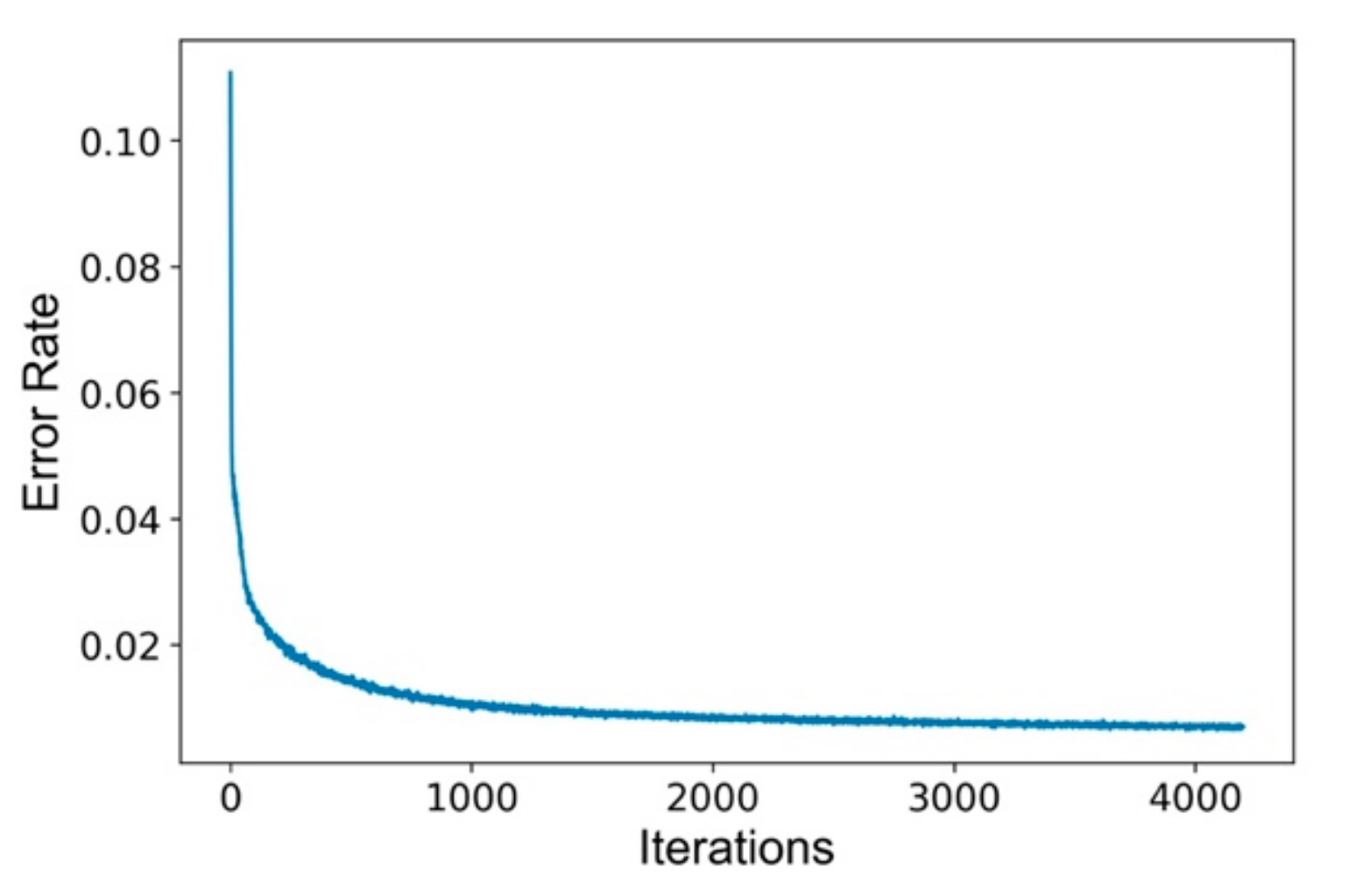
Since input data is preprocessed, the training of RBM model is first started. The original features of weekly load data have 168 dimensions so the tentative number of hidden layer neurons is set to {60,80,100,120} which will be determined based on subsequent clustering performance. Other neural network parameters are adjusted through training, which includes that the iteration upper limit is set to 4500 rounds, the momentum index equals 0.75 and the learning rate equals 0.0007. As the shown Silhouette Coefficient performance above in Table 1, the hidden layer feature is set to be 80-dimensional. With all the parameters determined, the training error curve with iterations is given as Figure 8.
The obtained 80-dimensional hidden features are clustered based on K-Means algorithm and 19 typical weekly load patterns are calculated. Figure 9 shows some of the typical load patterns.
It can be seen that most of the weekly load patterns show significant fluctuations in the cycle of 7 days a week. Figure 9a maintains load consumption peak during the daytime with 12:00 and 18:00 reaching the highest, which can be assumed as the catering industry power use. It can also explain that the top is jagged due to meal preparation, lunch break, etc. Figure 9b has large fluctuations every day with morning and evening reaching the peak, yet daytime utilization being relatively low. It can be supposed to be hospitality industry where customers leave in the morning and return in the evening. The daily load pattern in Figure 9c–f is quite simple, showing a typical nine-to-five load consumption mode during working days. It also changes with weekends and holidays, which can be presumed to be such industries as apartments, retails or educational institutions. These load patterns will be mentioned again in the next user analysis stages.
3.3. Two-Step User Clustering in Long-Term
With typical weekly load patterns obtained, the time scale conversion is performed and a two-step clustering is carried out to divide typical customer groups in long-term. Relying on Hierarchical coarse-grained clustering on user similarity matrix, a total of 10 main clusters are calculated. Continuously, the improved DBSCAN clustering is used for each main cluster to be reclassified which results in 16 fine-grained subclasses.
Table 2 shows the results of main clusters and their subclasses, where the bracket means there is more than one subclass. From the perspective of clustering effect, the accuracy of clustering can reach 87.5% according to the 16 standard commercial building types by DOE. In more detailed, several typical clusters with their load patterns will be introduced respectively in Figure 10, Figure 11 and Figure 12, where long-term user behavior is shown on the left and corresponding short-term load pattern is on the right in each subgraph.
User cluster 1: This cluster belongs to Full Service Restaurant and Quick Service Restaurant, containing 100 users with a completely identical load pattern. As shown in Figure 10, from the perspective of short term, the catering industry has business hours as the electricity consumption peak, of which lunch and dinner periods are the highest in particular. Since less electricity is consumed during meal preparation and afternoon rest periods, a jagged consumption mode with alternating peaks and valleys is formed. Moreover, analyzing in long-term, catering users are open all year round with the same load pattern maintained every day, except for the influence of summer time.
User cluster 3: Cluster 3 contains 42 typical users, which takes a proportion of 84% and represents the standard commercial building of Outpatient. As shown in Figure 11, outpatient clinics have an apparent habit that maintains 6 days as consumption peak and 1 day as valley in a week, except for several federal holidays. This is mainly because outpatient clinics will be closed during federal holidays and weekends while the urgent care clinics remain open and fully staffed 24 h a day, which leads to a significant reduce of electricity consumption amount but a preservation of wave shape during rests.
User cluster 4: This cluster contains a total of 50 users, of which 48 are typical users and only 2 are abnormal users, belonging to the classification of Warehouse. As shown in Figure 12, as a warehouse user, the goods are brought in and out every workday except for extra rests brought by holidays, which leads to a fixed weekly load pattern where there is high electricity consumption on weekdays but almost no consumption on weekends. Compared to educational institution users which will be mentioned next, warehouse has a minimum load limit to maintain normal operations and keep goods safe. Therefore, there will be a certain power load during the night while nearly no electricity is used in primary and secondary schools.
User cluster 6: This cluster looks exaggerated but has an accurate division where subclass1 has 45 users and subclass2 has 40 users, representing standard classification of Primary School and Secondary School respectively as Figure 13b,c. Taking the identical load pattern in Figure 13a into consideration, primary school users have extremely regular schedules with few differences between regions. In contrast, secondary school users’ behavior varies throughout the year due to the different regulations of different states. As a result of differences in holiday arrangements and weekend innovation activities, electricity consumption on weekends has a huge gap among secondary schools. Despite of this, different load patterns’ distance between each other is not that much, which can still lead to high similarities and be clustered into secondary school class anyway.
The power consumption behavior of other clusters is relatively stable, which will not be mapped due to space. Based on the analysis of typical cluster load pattern, we found out that Large Hotel and Small Hotel have basically no change in consumption mode throughout the year, which fits the distribution of higher power consumption in the morning and evening but lower in working hours and is consistent with the behavior of customers entering and leaving the hotel. Besides, Stand-alone Retail and Strip Mall maintain the same mode which runs at a high level every day with slight decline only on weekends. The difference between these two types is mainly concentrated in the Columbus Day, where retail users are operating normally while strip mall users will significantly increase their electricity consumption due to more holiday customers. Furthermore, Super Market users maintain high-load operation regardless of the day and forms the whole year consumption peak during the Thanksgiving day in particular.
In order to verify that the AUD-MTS method can calculate a user partition more precisely, we compare it with other common clustering algorithms, including Spectral Clustering, Agglomerative Clustering and K-Means algorithm. The pending data is users’ similarity matrix in long-term and algorithm parameters are selected by Silhouette Coefficient scores, with the measurement indicators defined in Section 3.1. Referring to the 16 standard commercial building categories, Table 3 below shows the performance of each algorithm on user behavior data.
It can be seen that the AUD-MTS method achieves the best performance on AMI, ARI and OutlierIndex while is slightly inferior to Agglomerative on V_measure. In general, both AUD-MTS and Agglomerative are implemented based on Hierarchical clustering, which performs better at the scene of user classification and gradual refinement. However, AUD-MTS gathers abnormal users into an additional cluster when users are subdivided, which leads to the V_measure indicator performing slightly worse than Agglomerative. Therefore, if the influence of outliers is taken into account, we can see that AUD-MTS method has a clear lead on OutlierIndex score.
4. Abnormal User Detection
4.1. Abnormal User Detection
When AUD-MTS reclassifies coarse-grained clustering results in long-term, the algorithm can also screen those points far away from cluster centers according to the density, which are defined as outliers.
Table 4 shows the details of detected abnormal users of each cluster. From the perspective of clusters, a total of 96 abnormal users are filtered out, which accounts for 12% of all users. Within them, there are abnormal users more or less except for the first cluster as catering industry. Considering anomaly causes, it is mainly attributed to holidays, climate zone and unknown reasons.
Holidays include federal holidays and special working days such as Black Friday, where there is usually a significant change in electricity consumption during that week.
The climate zone refers to various climate regions based on heating degree-days, average temperatures, precipitation and so on, which is defined by the U.S. Department of Energy. Different climate zones include Subarctic, Very Cold, Cold, Mixed-Humid, Mixed-Dry, Hot-Humid, Hot-Dry and Marine climate. The temperature and climate have significant differences among these regions, which will greatly affect user electricity consumption habits.
The last one is the unknown reason, of which users often generate irregular load pattern mutations in irregular time, which is quite different from typical users and hard to forecast. These users may be potential stealing users which would require follow ups with further checks.
Figure 14 shows the distribution of all abnormal users in the United States, where the deeper the color is, the more frequently abnormal users appear in the state. It can be clearly seen that the proportion of abnormal users in Hawaii and Alaska is extremely high due to the harsh climate and values in the states near Gulf of Mexico, such as Florida and Louisiana, are significantly higher than that in inland. This is mainly owing to the vast size of the United States and the huge climate differences among regions. For instance, the climate of southeastern coast is more variable and more abundant in precipitations than inland, which will affect users’ work, travel and consumption habits and eventually lead to different load consumption modes. Similarly, the Pacific coast has fewer abnormal users than Atlantic coast due to its mild marine climate even though they are both coastal areas.
As Figure 15 displayed below, the curve shows the impact of Holidays on annual user behaviors and weekly load patterns of both typical users and abnormal users of the class Strip Mall. It can be seen from the figure that abnormal users have sudden changes in consumption behavior at the 22nd week, 36th week and 41st week respectively, where there is a significant reduction in load consumption during these weeks. The reason is that during these three weeks there happens to be federal holidays including Memorial Day, Labor Day and Columbus Day, when stores are closed and employees have time off, resulting in the sharp shrink of electricity consumption.
Another example in Figure 16 shows how the climate zones influence consumption behaviors of Hotel users, where typical users come from Springfield, Illinois and abnormal users are from Marathon, Florida. Typical users maintain a consistent mode of a peak power usage at 08:00 and 21:00 and a relatively low load during daytime. However, Marathon City often experiences sudden changes of consumption behavior in May, August and September, when the electricity consumption is significantly reduced during morning and daytime and the reduction is close to 40% of the peak usage amount.
The specific cause of anomalies may be related to local climates. May to October is the rainy season of Marathon when monthly precipitation is above 100 mm and in particular, the average precipitation in August and September can reach 150 mm with precipitation days exceeding 15 days. During the rainy season, there are fewer customers visiting the hotel and the electricity consumption for lighting, cooling and cooking will drop significantly. Besides, those customers who checked in will also reduce their stay at the hotel during the daytime and get to workplaces as soon as possible, resulting in a further decline of the hotel’s electricity consumption.
4.2. Abnormal Behavior Causes and Strategies
- (a)
- Holiday
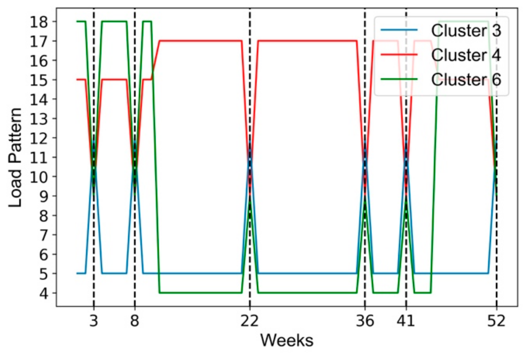
As Figure 17, we find that the time when user electricity consumption behavior changes has a large degree of coincidence, especially at the 3rd week, 8th week, 22nd week, 36th week, 41st week, and 52nd week shown in Figure 16. Most users experience a significant increase or decrease in power usage within a few days. An analysis of the dates reveals that these weeks mostly contain U.S. federal holidays, which will significantly change the consumption mode of users, including but not limited to, the following holidays: New Year’s Day, President’s Day, Memorial Day, Independence Day, Labor Day, Veterans Day, Thanksgiving Day and Christmas Day.
In response to this regular collective change in user behavior, power industry needs to make dispatching strategies in advance. For instance, power supply can be appropriately reduced during federal holidays for user groups such as offices and schools. The saved power could be allocated to supermarkets and hospitals that have significantly increased demand during holidays so as to achieve load balancing and reduce the occurrence of emergencies.
- (b)
- Climate Zone
As in the distribution map of abnormal users shown before, abnormal users are distributed among states quite unevenly due to large climate differences. In general, there are
- more abnormal users in coastal areas than in inland areas;
- more abnormal users on the east coast than on the Pacific coast;
- more abnormal users in both high and low latitudes than in the middle latitudes.
The temperature range in these areas is quite vast and the rainy season duration and precipitation has a magnitude difference, which will have a significant impact on electricity consumption habits of local users. However, if we abandon the national perspective and turn to each state instead, the users in the same city still have a fairly high similarity.
Due to the huge climate differences in various regions, it is necessary for each state government to formulate policies in conjunction with local situations, such as adjusting working hours during extreme weathers. At the same time, the power companies in each state should also analyze local climate characteristics, predict future load situation based on historical information and guide the users’ electricity usage behavior by designing demand side response. In a word, preparing for the possible coming changes in advance is the best way to avoid failure and overload.
- (c)
- Summer Time
In the process of analyzing user behavior changes in long-term, these two change modes shown below are quite attracting while the users corresponding to these are rarely classified as abnormal users. As shown in Figure 18, the sudden changes happen at the 11th week and the 45th week but there is not much difference in typical weekly load patterns before and after. It is found out that the peak-to-valley values are shifted by one hour with numerical values basically unchanged.
This is due to the implementation of summer time and winter time in the United States. With the aim of enjoying sunlight and saving lightning load, the summertime starts from the second Sunday of March and ends on the first Sunday of November every year. During this period, the time is adjusted one hour earlier. When RBM learns hidden features, this difference is captured by machine learning automatically and becomes a dimension of the load pattern division, which can distinguish whether users are affected by summer time or not.
4.3. Comparison
In order to verify that AUD-MTS method can detect abnormal users precisely and efficiently, we compare it with other common outlier detection algorithms including Local Outlier Factor (LOF) and Isolation Forest algorithm. LOF is an unsupervised outlier detection algorithm by measuring the local deviation of density of a given sample with respect to its neighbors. The Isolation Forest algorithm calculates the anomaly score by randomly selecting a feature and then randomly selecting a split value for the selected feature between the maximum and minimum values of the feature.
Ten rough user clusters calculated by K-Means coarse-grained clustering are selected as the experiment data and each of the clusters is subjected to LOF, IF and AUD-MTS for a secondary clustering respectively. The parameters used in this process are automatically adjusted by grid search with no additional variables involved. Since cluster 1 is a pure class with a completely identical load pattern, it will not be included and the performance of other nine clusters on OutlierIndex is given as Table 5.
As Figure 19, it can be seen that AUD-MTS can get the highest average score and the best performance in seven out of nine categories, which proves that it can get the most accurate abnormal user detection. What is more, in those scenes where sub-cluster partitioning is required such as cluster 5 and cluster 6, AUD-MTS is clearly better than LOF and IF. This is because LOF and IF can only detect outliers according to scores, which is impossible to distinguish whether the user cluster needs to be more detailed. The sub-cluster users will be classified into one category or all of them are identified as outliers, while AUD-MTS can calculate subclasses from a fine-grained dimension.
5. Conclusions
This paper proposes an abnormal user detection approach based on power load multi-step clustering with multiple time scales (AUD-MTS), which can screen abnormal users by analyzing power load and user behavior in both short-term and long-term. It was verified on power load data set of the United States that AUD-MTS classified the whole users into 10 categories and 16 sub-categories and screened 12% of them as abnormal users, which is more precisely and efficiently than other common clustering algorithms and outlier detection algorithms. We found that abnormal users have a consistent distribution in both time and space dimension, where those belonging to different types have completely different reactions to holidays and natural changes. Therefore, we summarized three possible causes including holiday, climate zone and summer time that may lead to unusual behavior changes and discussed strategies respectively. However, more open-source datasets are required to show the stability and generalization capabilities of the proposed model. This will be our future work.
Power load data is still the most valuable data used for customer profile and behavior analysis. We will continually optimize the method and analyze Chinese user behaviors and abnormal users in China by using load data set of China furthermore.
Author Contributions
R.L. designed the algorithm, performed the experiments, and prepared the manuscript as the first author. M.G. and Y.Z. assisted the project and managed to obtain the load data. F.Y. and B.W. helped to Writing-Review & Editing.
Funding
State Grid Corporation of China (520940180016).
Acknowledgments
This work was supported by the State Grid Corporation of China (520940180016).
Conflicts of Interest
The authors declare no conflict of interest.
References
- Blumsack, S.; Fernandez, A. Ready or not, here comes the smart grid! Energy 2012, 37, 61–68. [Google Scholar] [CrossRef]
- Kovacic, Z.; Giampietro, M. Empty promises or promising futures? The case of smart grids. Energy 2015, 93, 67–74. [Google Scholar] [CrossRef]
- Chicco, G. Overview and performance assessment of the clustering methods for electrical load pattern grouping. Energy 2012, 42, 68–80. [Google Scholar] [CrossRef]
- McLoughlin, F.; Duffy, A.; Conlon, M. A clustering approach to domestic electricity load profile characterisation using smart metering data. Appl. Energy 2015, 141, 190–199. [Google Scholar] [CrossRef] [Green Version]
- Panapakidis, I.P.; Papadopoulos, T.A.; Christoforidis, G.C.; Papagiannis, G.K. Pattern recognition algorithms for electricity load curve analysis of buildings. Energy Build. 2014, 73, 137–145. [Google Scholar] [CrossRef]
- Chuan, L.; Ukil, A. Modeling and validation of electrical load profiling in residential buildings in Singapore. IEEE Trans. Power Syst. 2015, 30, 2800–2809. [Google Scholar] [CrossRef]
- Tang, X.; Hasan, K.N.; Milanovic, J.V.; Bailey, K.; Stott, S.J. Estimation and validation of characteristic load profile through smart grid trials in a medium voltage distribution network. IEEE Trans. Power Syst. 2018, 33, 1848–1859. [Google Scholar] [CrossRef]
- Li, X.; Bowers, C.P.; Schnier, T. Classification of energy consumption in buildings with outlier detection. IEEE Trans. Ind. Electron. 2010, 57, 3639–3644. [Google Scholar] [CrossRef]
- Labeeuw, W.; Deconinck, G. Residential electrical load model based on mixture model clustering and markov models. IEEE Trans. Ind. Inform. 2013, 9, 1561–1569. [Google Scholar] [CrossRef]
- Mets, K.; Depuydt, F.; Develder, C. Two-stage load pattern clustering using fast wavelet transformation. IEEE Trans. Smart Grid 2016, 7, 2250–2259. [Google Scholar] [CrossRef]
- Chicco, G.; Ilie, I.S. Support vector clustering of electrical load pattern data. IEEE Trans. Power Syst. 2009, 24, 1619–1628. [Google Scholar] [CrossRef]
- Chicco, G.; Ionel, O.M.; Porumb, R. Electrical load pattern grouping based on centroid model with ant colony clustering. IEEE Trans. Power Syst. 2013, 28, 1706–1715. [Google Scholar] [CrossRef]
- Zhang, T.; Zhang, G.; Lu, J.; Feng, X.; Yang, W. A new index and classification approach for load pattern anal- ysis of large electricity customers. IEEE Trans. Power Syst. 2012, 27, 153–160. [Google Scholar] [CrossRef]
- Villar-Rodriguez, E.; Del Ser, J.; Oregi, I.; Bilbao, M.N.; Gil-Lopez, S. Detection of non-technical losses in smart meter data based on load curve profiling and time series analysis. Energy 2017, 137, 118–128. [Google Scholar] [CrossRef] [Green Version]
- Capozzoli, A.; Piscitelli, M.S.; Brandi, S.; Grassi, D.; Chicco, G. Automated load pattern learning and anomaly detection for enhancing energy management in smart buildings. Energy 2018, 157, 336–352. [Google Scholar] [CrossRef]
- Seem, J.E. Using intelligent data analysis to detect abnormal energy consumption in buildings. Energy Build. 2007, 39, 52–58. [Google Scholar] [CrossRef]
- Tang, G.; Wu, K.; Lei, J.; Bi, Z.; Tang, J. From landscape to portrait: A new approach for outlier detection in load curve data. IEEE Trans. Smart Grid 2014, 5, 1764–1773. [Google Scholar] [CrossRef]
- Wang, J.; Xiong, S. A hybrid forecasting model based on outlier detection and fuzzy time series a case study on hainan wind farm of china. Energy 2014, 76, 526–541. [Google Scholar] [CrossRef]
- Chicco, G.; Napoli, R.; Piglione, F. Comparisons among clustering techniques for electricity customer classification. IEEE Trans. Power Syst. 2006, 21, 933–940. [Google Scholar] [CrossRef]
- Chicco, G.; Napoli, R.; Piglione, F.; Postolache, P.; Scutariu, M.; Toader, C. Load pattern-based classification of electricity customers. IEEE Trans. Power Syst. 2004, 19, 1232–1239. [Google Scholar] [CrossRef]
- Chicco, G.; Napoli, R.; Postolache, P.; Scutariu, M.; Toader, C. Customer characterization options for improving the tariff offer. IEEE Trans. Power Syst. 2003, 18, 381–387. [Google Scholar] [CrossRef]
- Viegas, J.L.; Vieira, S.M.; Melcio, R.; Mendes, V.; Sousa, J.M. Classification of new electricity customers based on surveys and smart metering data. Energy 2016, 107, 804–817. [Google Scholar] [CrossRef]
- Quilumba, F.L.; Lee, W.-J.; Huang, H.; Wang, D.Y.; Szabados, R.L. Using smart meter data to improve the accuracy of intraday load forecasting considering customer behavior similarities. IEEE Trans. Smart Grid 2015, 6, 911–918. [Google Scholar] [CrossRef]
- Teeraratkul, T.; O’Neill, D.; Lall, S. Shape-based approach to household electric load curve clustering and prediction. IEEE Trans. Smart Grid. 2017, 9, 5196–5206. [Google Scholar] [CrossRef]
- Yu, Z.J.; Haghighat, F.; Fung, B.C.; Morofsky, E.; Yoshino, H. A methodology for identifying and improving occupant behavior in residential buildings. Energy 2011, 36, 6596–6608. [Google Scholar] [CrossRef] [Green Version]
- Gouveia, J.P.; Seixas, J.; Mestre, A. Daily electricity consumption profiles from smart metersproxies of behavior for space heating and cooling. Energy 2017, 141, 108–122. [Google Scholar] [CrossRef]
- Ma, Z.; Yan, R.; Nord, N. A variation focused cluster analysis strategy to identify typical daily heating load profiles of higher education buildings. Energy 2017, 134, 90–102. [Google Scholar] [CrossRef] [Green Version]
- Ahmad, T.; Chen, H. Potential of three variant machine-learning models for forecasting district level medium term and long-term energy demand in smart grid environment. Energy 2018, 160, 1008–1020. [Google Scholar] [CrossRef]
- Huang, S.; An, H.; Wen, S.; An, F. Revisiting driving factors of oil price shocks across time scales. Energy 2017, 139, 617–629. [Google Scholar] [CrossRef]
- Pan, Z.; Guo, Q.; Sun, H. Interactions of district electricity and heating systems considering time-scale characteristics based on quasisteady multi-energy flow. Appl. Energy 2016, 167, 230–243. [Google Scholar] [CrossRef]
- Jaln, M.L.; Baquerizo, A.; Losada, M.A. Optimization at different time scales for the design and management of an oscillating water column system. Energy 2016, 95, 110–123. [Google Scholar] [CrossRef]
- Bhattarai, B.P.; Myers, K.S.; Bak-Jensen, B.; Paudyal, S. Multi-time scale control of demand flexibility in smart distribution networks. Energies 2017, 10, 37. [Google Scholar] [CrossRef]
- Abdon, A.; Zhang, X.; Parra, D.; Patel, M.K.; Bauer, C.; Worlitschek, J. Techno-economic and environmental assessment of stationary electricity storage technologies for different time scales. Energy 2017, 139, 1173–1187. [Google Scholar] [CrossRef]
- Zhao, Z.; Yang, P.; Guerrero, J.M.; Xu, Z.; Green, T.C. Multiple-time-scales hierarchical frequency stability control strategy of medium-voltage isolated microgrid. IEEE Trans. Power Electron. 2016, 31, 5974–5991. [Google Scholar] [CrossRef]
- Yao, Y.; Huang, L.; Sharma, A.B.; Golubchik, L.; Neely, M.J. Power cost reduction in distributed data centers: A two-time-scale approach for delay tolerant workloads. IEEE Trans. Parallel Distrib. Syst. 2014, 25, 200–211. [Google Scholar]
Figure 1.
The overall process of AUD-MTS approach.

Figure 2.
The network structure of Restricted Boltzmann Machine (RBM) model.

Figure 3.
User data conversion process with label generation and similarity matrix calculation.

Figure 4.
User data model conversion from short-term to long-term.

Figure 5.
The algorithm flowchart of user behavior analysis in long-term.

Figure 6.
Algorithm procedure.

Figure 7.
Examples of weekly power load curve (left) and annual power load curve (right).

Figure 8.
RBM model training error rate with iterations.

Figure 9.
Six typical local patterns in short-term: (a) daytime highest; (b) morning and evening; (c) lunch time highest; (d) normal working day 1; (e) normal working day 2; (f) normal working day 3.
Figure 9.
Six typical local patterns in short-term: (a) daytime highest; (b) morning and evening; (c) lunch time highest; (d) normal working day 1; (e) normal working day 2; (f) normal working day 3.

Figure 10.
Typical user behaviors of catering industry (left) and corresponding load patterns in short-term (right).
Figure 10.
Typical user behaviors of catering industry (left) and corresponding load patterns in short-term (right).

Figure 11.
Typical user behaviors of Outpatient (left) and corresponding load patterns in short-term (right).
Figure 11.
Typical user behaviors of Outpatient (left) and corresponding load patterns in short-term (right).

Figure 12.
Typical user behaviors of Warehouse (left) and corresponding load patterns in short-term (right).
Figure 12.
Typical user behaviors of Warehouse (left) and corresponding load patterns in short-term (right).

Figure 13.
Typical user behaviors of Primary School (b), Secondary School (c) and corresponding load patterns in short-term (a).
Figure 13.
Typical user behaviors of Primary School (b), Secondary School (c) and corresponding load patterns in short-term (a).


Figure 14.
The distribution heat map of detected abnormal users referring to each state.

Figure 15.
The impact of holidays on Strip Mall users with user behavior (left) and load patterns (right).
Figure 15.
The impact of holidays on Strip Mall users with user behavior (left) and load patterns (right).

Figure 16.
The impact of climate zones on Hotel users of Illinois and Florida with user behavior (left) and load patterns (right).
Figure 16.
The impact of climate zones on Hotel users of Illinois and Florida with user behavior (left) and load patterns (right).

Figure 17.
Special time points of abnormal user behavior changes happening.

Figure 18.
The influence of summer time from 11st week to 45th week.

Figure 19.
OutlierIndex score performance of three algorithms on each cluster.


Table 1.
Silhouette Coefficient performance of clustering based on various hidden layer neurons.
| Hidden Layer Neurons | 120 | 100 | 80 | 60 |
|---|---|---|---|---|
| Silhouette Coefficient | 0.4359 | 0.4559 | 0.4654 | 0.4613 |
Table 2.
User fine-grained classification details of each cluster.
| Results (Cluster) | C1 | C2 | C3 | C4 | C5 | C6 | C7 | C8 | C9 | C10 |
|---|---|---|---|---|---|---|---|---|---|---|
| Total | 100 | 50 | 50 | 50 | 150 | 100 | 50 | 100 | 100 | 50 |
| Main Class | 100 | 46 | 42 | 48 | 50 | 45 | 34 | 88 | 69 | 36 |
| Subclasses | 0 | 0 | 0 | 0 | {32,48} | 40 | 0 | 0 | {5,11} | {10} |
| Outliers (%) | 0% | 8% | 16% | 4% | 13.3% | 15% | 32% | 12% | 15% | 8% |
Table 3.
Performance of different clustering algorithms referring to defined indicators.
| Algorithm | Cluster Number | V_measure | AMI | ARI | OutlierIndex |
|---|---|---|---|---|---|
| AUD-MTS | 16 | 0.8214 | 0.7848 | 0.6578 | 0.8731 |
| Spectral Clustering | 15 | 0.7155 | 0.6087 | 0.3366 | −0.1475 |
| Agglomerative Clustering | 14 | 0.8411 | 0.7731 | 0.6407 | 0.6649 |
| K-Means | 16 | 0.7242 | 0.6240 | 0.3594 | 0.3496 |
Table 4.
Abnormal user detection details of each cluster based on possible causes.
| Anomalies (Cluster) | C1 | C2 | C3 | C4 | C5 | C6 | C7 | C8 | C9 | C10 | Total (%) |
|---|---|---|---|---|---|---|---|---|---|---|---|
| Abnormal Users | 0 | 4 | 8 | 2 | 20 | 15 | 16 | 12 | 15 | 4 | 100% |
| Holidays | 0 | 0 | 8 | 1 | 7 | 10 | 5 | 8 | 15 | 4 | 60.4% |
| Climate Zone | 0 | 2 | 0 | 1 | 6 | 2 | 7 | 3 | 0 | 0 | 21.9% |
| Unknown | 0 | 2 | 0 | 0 | 7 | 3 | 4 | 1 | 0 | 0 | 17.7% |
Table 5.
The comprehensive performance of three outlier detection methods.
| Algorithm | Outlier Number | Outerlier Rate (%) | OutlierIndex (avg) |
|---|---|---|---|
| AUD-MTS | 96 | 12% | 1.406 |
| LOF | 85 | 10.625% | 1.160 |
| IsolationForest | 162 | 20.25% | 1.246 |
© 2019 by the authors. Licensee MDPI, Basel, Switzerland. This article is an open access article distributed under the terms and conditions of the Creative Commons Attribution (CC BY) license (http://creativecommons.org/licenses/by/4.0/).
Share and Cite
MDPI and ACS Style
Lin, R.; Yang, F.; Gao, M.; Wu, B.; Zhao, Y. AUD-MTS: An Abnormal User Detection Approach Based on Power Load Multi-Step Clustering with Multiple Time Scales. Energies 2019, 12, 3144. https://doi.org/10.3390/en12163144
AMA Style
Lin R, Yang F, Gao M, Wu B, Zhao Y. AUD-MTS: An Abnormal User Detection Approach Based on Power Load Multi-Step Clustering with Multiple Time Scales. Energies. 2019; 12(16):3144. https://doi.org/10.3390/en12163144
Chicago/Turabian StyleLin, Rongheng, Fangchun Yang, Mingyuan Gao, Budan Wu, and Yingying Zhao. 2019. "AUD-MTS: An Abnormal User Detection Approach Based on Power Load Multi-Step Clustering with Multiple Time Scales" Energies 12, no. 16: 3144. https://doi.org/10.3390/en12163144
Note that from the first issue of 2016, this journal uses article numbers instead of page numbers. See further details here.