Economic Analysis of HRES Systems with Energy Storage During Grid Interruptions and Curtailment in Tamil Nadu, India: A Hybrid RBFNOEHO Technique

Abstract

This work presents an economic analysis of a hybrid renewable energy source (HRES) integrated with an energy storage system (ESS) using batteries with a new proposed strategy. Here, the HRES system comprises wind turbines (WT) and a photovoltaic (PV) system. The hybrid WT, PV and energy storage system with battery offer several benefits, in particular, high wind generation utilization rate, and optimal generation for meeting supply-demand gaps. The real recorded data of various parameters of a 22 KV hybrid ‘Regen’ feeder of 110/22 KV Vagarai Substation of TANTRANSCO in Palani of Tamilnadu in India was gathered, studied for the entire year of 2018, and utilized in this paper. The proposed strategy is the hybridization of two algorithms called Radial Basis Function Neural Network (RBFNN) and Oppositional Elephant Herding Optimization (OEHO) named the RBFNOEHO technique. With the help of RBFNN, the continuous load demand required for the HRES and be tracked. OEHO is used to optimize a perfect combination of HRES with the predicted load demand. The aim of the proposed hybrid RBFNOEHO is to study the cost comparison of the HRES system with the existing conventional base method, energy storage method (ESS) with batteries and with HOMER. The proposed Hybrid RBFNOEHO technique is evaluated by comparing it with the other techniques; it is found that the proposed method yields a more optimal solution than the other techniques.

1. Introduction

In the present scenario, the energy demand is managed with both renewable and non-renewable sources in most of the countries around the world. More quantum generation of green energy than fossil fuels is the need of the hour due to both the cost factor as well as the mitigation of global warming. At the same time, the optimum production of green energy even during interruptions is a challenging task. Hence, a study of the economic analysis on this subject is more important. The Sun is the prime source of all energies and power. Heat and light, being the primary forms of solar energy are transformed and absorbed by the environment in various ways for sustainability; this has been reviewed in [1,2,3,4]. A review on the relationships between energy transformation from renewable energy sources such as wind and solar with climate change mitigation has been presented in [5]. This, in turn, helps to mitigate greenhouse gas emissions and reduce global warming as has been explained in [6], along with the anticipated patterns of future energy use. A review on the scope of CO₂ mitigation through various renewable energy gadgets has been presented [7]. In general, wind energy is caused by airflow and solar energy is caused by irradiation. Hence, the amount of harvestable renewable energy predicted for a particular time span might not be accurate. In addition, renewable energy sources are intermittent, fluctuating and non-continuous. Many unsatisfactory issues due to implementation of renewable electricity systems alone have been addressed in detail [8]. Voltage, frequency, and waveform are the three important affecting factors of the ‘power quality’ of the distribution network, due to the synchronization of the generation from renewable energy sources into the power grid [9]. It has been reported that this could also affect the scheduling scheme, in turn, hence further affecting the normal operation of the distribution network. The grid synchronization of the power is discussed in detail by [10,11]. Energy storage technologies using batteries in hybrid wind power operations is analyzed in [12,13]. The characteristics and a comparison of energy storage systems have been reviewed in [14]. The need for energy storage in active distribution networks in spite of the uncertainty of wind power distributed generation is discussed in [15].

In this context, the study of the integration of hybrid renewable energy systems with the power grid is essential. The main essence of the energy storage is nothing but the properties of its ‘space transfer energy’ for stable operation of the power grid and thereby to improve the power quality. In [16], an OPF control of HRES with energy storage was discussed, and the achievement of a better dynamic response due to energy storage has been proved.

In recent years, a number of nature-inspired metaheuristic evolutionary algorithms have been studied in depth and are being applied to solve different types of optimization problems. Examples of such algorithms are the Genetic Algorithm (GA) [17,18,19], Biogeography-based Optimization (BBO) [20], Particle Swarm Optimization (PSO) [21,22], Artificial Bee Colony (ABC) [23], Different Evolution (DE) [24], Bacterial Foraging Optimization (BFO) [25], Ant Colony Optimization (ACO) [26], Cuckoo Search (CS) [27], Honey Bee Mating Optimization (HBMO) [28], BAT Algorithm [29], etc. These different types of algorithms are often being used to solve the various engineering problems that arise in different fields. Numerous research works are available in the literature for optimum power flow management using solar energy and wind energy transformation applying different techniques in different parts of the world. The steps taken by the Korea Electric Power Corporation (KEPCO) to develop a Renewable Energy Map (REM) in South Korea have been reviewed in [30]. In addition, they have explained the steps taken for optimal location identification for a renewable complex without violating any reliability standards.

An effective assessment approach to non-renewable energy sources has been developed in Taiwan; the country is dependent on the importation of energy, with more than 99% coming from foreign countries, as discussed in [31]. In [32], the many problems and challenges faced by China’s wind power industry are reviewed in detail. A comprehensive assessment was presented to discuss China’s wind power industry, power demand, cost and distribution of wind power. In [33] it was reported that the wind power access to power grids could have a great influence on the power stability and power quality of the distribution network of Henan Province in China.

In [34], the availability of the abundant solar radiation and the challenges for utilizing it for solar irrigation in Bangaladesh has been reviewed. In [35] the availability of RES and the present technologies practiced in Bangladesh have been briefed with conclusions for the implementation of systematic changes from conventional to the non-conventional (renewable) methods to obtain benefits for the whole nation.

This work focuses on an economic analysis to integrate an energy storage system (ESS) using batteries along with different hybrid renewable energy source (HRES) devices using the proposed strategy. Here, the HRES system comprises wind turbines (WT) and a photovoltaic (PV) system. The proposed strategy is the hybridization of two algorithms called Radial Basis Function Neural network (RBFNN) explained by [36] and Oppositional Elephant Herding Optimization (OEHO) described by [37], together named the RBFNOEHO technique.

Reference [38] has proposed an optimal energy management for a grid-connected PV-WT, MT and ESS hybrid energy system utilizing the ANFMDS approach and Homer. The technique has analyzed various load demands of the microgrid.

In the proposed study, a detailed analysis based on real data is discussed to insist on the need for an energy storage system to avoid the wastage of the production and utilization of green energy. Beneficially and economically; in particular, generation during various types of ‘grid interruption’ and utilization during the ‘peak’ hours and ‘maintenance periods’ of the solar and wind electric generators are studied. The research work is a comparative economic analysis of HRES without using energy storage and battery storage during grid interruption and curtailment. Curtailment has been a major concern for RES. Curtailment can be defined as a reduction in the output of a generator from what it could otherwise produce given the available resources (e.g., wind or sunlight), typically on an involuntary basis. Curtailment occurs when a transmission system operator issues an instruction to limit the energy output of a specific or a group of RES generators. There is lot of evidence for the incidence of curtailment across many states in India. Curtailment is heavily influenced by local factors, such as the status of the grid infrastructure near an RE generation site and resource variability at those sites. There is considerable variation in the quantum of curtailment across months, states, and even districts in a state, so there is a need to solve the issue during grid interruptions and curtailment using HRES combined with the optimal storage system.

In this paper, an existing Hybrid Renewable Energy Source (HRES) comprising a wind power generation and solar power generation system in a single 22 KV feeder at Vagarai located in the Palani Division in the Dindigul Circle of TANGEDCO in Tamil Nadu, India has been chosen for study. This dissertation focuses on an economic analysis to integrate the hybrid renewable energy sources (HRES) with an energy storage system (ESS) using batteries in the proposed strategy. Here, the HRES system comprises wind turbines (WT) and a photovoltaic (PV) system. The proposed strategy is the hybridization of two algorithms called Radial Basis Function Neural Network (RBFNN) and Oppositional Elephant Herding Optimization (OEHO) named the RBFNOEHO technique. The rest of the paper is organized as follows: Section 2 describes the topography of Tamil Nadu state. Section 3 contains a description of the chosen area. Section 4 describes the objective function formulation. Section 5 portrays the system configuration of HRES system. Section 6 postulates the economic analysis of battery storage system for HRES system using the proposed hybrid strategy. Section 7 defines the real data and simulation results and a discussion. Section 8 concludes the manuscript.

2. Topography of the State of Tamil Nadu

In general, in India, the Sun is visible on sunny days at 6.00 a.m. in the morning and disappears at 6.00 p.m. The solar insulation varies with seasons. However, in general, the peak of the irradiation during sunny days occurs between 7.30 a.m. and 4.00 p.m. The energy demand can be fulfilled by solar energy only during daytime hours. On the other hand, wind energy is available in the southwest monsoon months of May through September in the peninsula and Tamil Nadu. The rest of the months there will be poor generation from wind due to lull periods or shorter generation periods. The energy balance for the entire day and night and throughout the year by the hybrid system alone is very difficult and it is not at all possible. The coordinates of the location of Thoppampatti village and Vagarai village in Palani, India are 10.5844° N, 77.5727° E. The average and maximum wind speed and wind gust over the years in Palani, India as described in [39] are shown in Figure 1.

The average sun hours and sun days over the years in Palani, India is shown in Figure 2, as described in [39].

3. Description of the Chosen Area

An existing hybrid system with both solar and wind generation combined and formed as 22 KV feeders and fed into 110/22 KV Vagarai Substation, in the Palani Division in the Dindigul Circle of TANGEDCO in the State of Tamil Nadu of India has been chosen for our study purposes. The presentation of the real data and analysis in this section will give the real picture of the present scenario and the need for energy storage for economical and beneficial usage of the green energy to meet the entire “Demand” requirement with the limited utilization of conventional energy. The switchyard arrangement of the 22 KV hybrid feeders in the 110/22 KV Vagarai SS is shown in Figure 3.

4. Objective Function Formulation

The existing 22 KV Vagarai feeder consists of one standalone 1.5 MW wind turbine (W₁), and one 1.5 MW wind turbine (W₂-_PV) combined in a hybrid configuration with a 0.300 MW solar PV system and one standalone 2.8 MW wind turbine (W₃). The cost of the entire system and the initial erection and commission cost is fixed. The objective function, which has to be minimized, can be expressed as follows:

$$Min\hspace{0.17em}(AC)=⎣N_{PV}{C}_{PV}+N_{WT}{C}_{WT}+P_{ESS}{C}_{ESS}-C_{gs}+C_{gp}⎦$$

(1)

where, AC is the annualized cost of the system. The annualized total costs of PV, WT and ESS are represented as $C_{PV},C_{WT}$ and $C_{ESS}$. The total price ($/year) of electricity purchased from the grid annually is denoted as $C_{gp}$ and the total price of electricity sold to the grid ($/year) annually is $C_{gs}$. The annualized cost of each component comprises several parts, that is, annualized capital cost, and annualized operational and annualized replacement cost.

The entire hybrid system comprises several components and the cost of the replacement of components during normal wear and tear and major breakdown is the running cost for operations and maintenance. The salary ofthe operational crew and miscellaneous costs like taxes on land and maintenance of the control room building is also included in the running cost. It also includes the cost ofpurchasing power for the operation of the wind turbines, when synchronized withthe grid. The system with the lowest cost would be classified as possessing the optimal strategy; it should overcome the constraints and one should measure the ‘per unit’ cost by dividing the total cost and the generation units in KWHr. In the proposed study, the production of power is the total supply of power to the grid at the instance of generation and the stored energyfed back, generated during predictable interruption periods. Hence when measuring per unit cost by dividing the total cost and the generation units in KWHr, it will be less when compared to the cost of the system without energy storage:

$$Max(Gen)=E_{W1}+E_{W2-PV}+E_{W3}-E_{\mathrm{Im}port-W1}-E_{\mathrm{Im}port-W2-PV}-E_{\mathrm{Im}port-W3}$$

(2)

$$Min(Cost)=C_{W1}+C_{W2-PV}+C_{W3}-C_{\mathrm{Im}port-W1}-C_{\mathrm{Im}port-W2-PV}-C_{\mathrm{Im}port-W3}$$

(3)

Here, the export of energy from the wind turbine (W₁) is denoted as E_W1, the export of energy from wind turbine (W₂) plus solar Photo Voltaic (PV) is denoted as (E_W2-PV) and the export of energy from the wind turbine (W₃) is denoted as E_W3. C_W1 is the cost of the sale of power to grid due to the standalone 1.5 MW wind turbine. C_W2PV is the cost of the sale of power to the grid due to the hybrid 1.5 MW wind turbine combined with the 0.300 MW solar PV systems and C_W3 is the cost of the sale of power to the grid due to the standalone 2.8 MW wind turbine.

By substituting the real data of the energy supplied to the grid through the 22 KV hybrid feeder of the 110 KV Vagarai SS, into the expressions of (2) and (3), will become:

$$Max(Gen)=3016380+3362200+6570120-10800-12420-11960=12913520\hspace{0.17em}KWHr$$

(4)

$$Min(Cost)=144786.24+161385.60+354786.48-518.40-596.16-645.84=659198\hspace{0.17em}\$$$

(5)

In the existing grid-connected hybrid system, without any energy storage, the cost per unit sold without any storage for the year 2018 in the 22 KV hybrid feeder, considering all interruption periods is:

$$C_{actual}=Min\hspace{0.17em}(Cost)/Max\hspace{0.17em}(Gen)$$

(6)

By substituting the real data of the net energy sold and the net cost towards supply of energy in (6), one gets the following expression:

$$C_{actual}=659198/12913520=0.05104=0.051\hspace{0.17em}\$$$

(7)

Hence, the annual average net cost of the energy sold to grid during the year 2018 without any storage system during the interruptions is worked out to be $0.051.

In the first operational segment, the entire load of the 110 KV Vagarai SS is fully served by the connected hybrid feeder, which consists of three WTz and a 0.300 KW solarPV unit:

$$P_{W1}(t)+P_{W2-PV}(t)+P_{W3}(t)=P_{Load}$$

(8)

In the second operational segment, the entire load is fully served by the connected hybrid feeder, which consists of three WTsz and the 0.300 KW solar PV system, when they are equal and higher than the load demand:

$$P_{W1}(t)+P_{W2-PV}(t)+P_{W3}(t)>P_{Load} \mathrm{or} P_{W1}(t)+P_{W2-PV}(t)+P_{W3}(t)\ge P_{Load}$$

(9)

The remaining power would be sent to the grid.

In the third operational segment, the load can be partly served by the connected hybrid feeder, which consists of three WTs and a 0.300 KW solar PV system, is less than the load demand:

$$P_{W1}(t)+P_{W2-PV}(t)+P_{W3}(t)<P_{Load}$$

(10)

5. System Configuration of the HRES System

In this section, the system configuration of the HRES system is explained. The PV panel is connected with a rectifier to deliver alternating current. The proposed combination of the WT-PV system will act as a power injection system to the power grid and does not have the features needed to apply any sort of power quality control on the generated power. The output power of the WT is directly delivered by means of the AC grid to the distribution side. The output power produced by the solar panels is fed into the grid through the DC-AC converter. A bidirectional charge controller carries out the functions of charging and discharging the battery and thus performing both the AC-DC conversion and voltage boosting. The non-continuous availability of the renewable sources would hinder a system not equipped for gathering the power dispatch standards of the load dispatch centers. Likewise, during periods of high wind, the wind turbines are forced to shut down to safeguard the equipment. Coordinating the battery with the renewable energy source devices will enable to store the excess energy and it could be used beneficially during peak power demand periods, thus improving the system reliability. It additionally enables the storage of energy duringperiods when low demand exists, so that it can be better utilized during the peak load periods. The system configuration of the HRES system in the proposed strategy is shown in Figure 4.

Photovoltaic systems and wind turbines are non-dispatchable resources. The battery system is anenergy storage device. In the proposed approach, in the light of the annualized capital and replacement cost the objective functions are resolved. Along these lines, the optimal operation is accomplished when the objective of maximized revenues and minimized usage of HRES is fulfilled.

6. Economic Analysis of Battery Storage System for HRES System Using Hybrid Strategy

In this section, the proposed strategy for the economic analysis of battery storage system for the HRES systemis described. The proposed strategy is the incorporation of Radial Basis Function Neural Network (RBFNN) and Oppositional Elephant Herding Optimization (OEHO) named RBFNOEHO. RBFNN can be regarded as a feed-forward network composed with three layers of neurons [36]. The EHO algorithm is developed from the natural behavior of elephant herding [37]. Figure 5 portrays the procedure of economic analysis of the proposed system.

In order to accelerate the convergence rate and performance, the EHO is enhanced with the concept of oppositional-based learning (OBL). With the help of RBFNN, the required load demand for the HRES system is continuously tracked. With the consideration of the predicted load demand, OEHO is optimized for the HRES perfect combination. The involvement of the annualized capital cost and replacement cost of the HRES system is the main objective of the proposed methodology. The constraint is the renewable energy sources accessibility, power demand and storage elements state of charge. The systematic process of RBFNN and OEHO are discussedin the following section.

6.1. Prediction of Load Demand Using RBFNN

RBFNN is an artificial neural network. In the field of mathematical modelling, the proposed artificial neural network uses radial basis functions as activation functions. The first layer is called the input layer. It consists of the source nodes for the input data. The second layer is the single hidden layer in the network. It is made up of the radial basis functions. The nonlinear transformation is applied by these functions from the input layer into the hidden layer. The third layer is called the output layer. The output layer of the network is a linear combination of radial basis functions of the inputs and neuron parameters.

Here, the RBFNN is trained by the target power demand with the appropriate input time intervals of the day. To establish the proposed approach, the selection of the input variables to each node in the first layer and the output is computed using the Gaussian membership function.

Based on these corresponding inputs and the output values the RBFNN is trained. The structure and the training process of the ANFIS are describedas follows:

Step 1: The Input Vector. In the input layer of the network, the input vector $a$ is applied. In the proposed approach, the time interval $T$ is the input of the network, load demand are the output of the network. Then the equation for the input vector is given by:

$$a={\left[a_1\hspace{0.17em}\hspace{0.17em}\hspace{0.17em}{a}_2\cdots \hspace{0.17em}\hspace{0.17em}{a}_p\hspace{0.17em}\right]}^T$$

(11)

Here, a represents the input vector of the RBFNN.

Step 2: The RBF Neurons. From the training set, each RBF neuron stores a ‘prototype’ vector, which is one of the vectors. Each RBF neuron compares the input vector to its prototype, and outputs a value between 0 and 1 which is a measure of similarity. Output of the RBF neuron will be 1 if the input is equal to the prototype. The value of the neuron’s response is called its ‘activation’ value. The prototype vector is called neuron’s ‘centre’.

Step 3: The Output Nodes. The output of the network consists of set of nodes; each output node computes a score sort for the associated category. Typically, by assigning the input to the category with the highest score a classification decision is made. From every RBF neuron, a score is computed by taking a weighted sum of the activation values. With each of the RBF neurons, an output node associates a weight value by weighted sum and before adding it to the total response, it multiplies the neuron’s activation by this weight. Every output node has its own set of weights for a different category because each output node is computing the score. Output node give positive weight to the RBF neurons and negative weight is shared to the others.

Step 4: RBF Neuron Activation Function. In between the input and its prototype vector, each RBF neuron computes a measure of the similarity. Input vectors are similar to the prototype, which returns a result closer to 1. There are different possible choices of similarity functions based on Gaussian. The equation for the Gaussian with a one-dimensional input is postulated as follows:

$$f(a)=\frac{1}{\alpha \sqrt{2\pi }}{e}^{-\frac{{\left(a-\beta \right)}^2}{2{\alpha }^2}}$$

(12)

Here, input can be represented as $a$, mean as $\beta$, standard deviation can be represented as α. The RBF neuron activation function is slightly different, and is typically written as:

$$\psi (a)=e^{-\eta \Vert a-\beta \Vert }{}^2$$

(13)

Here, β is the mean of the distribution in the Gaussian distribution. After completing the algorithm, the RBFNN generates the load demand. Then the predicted values are used as the input of OEHO to get the optimal energy management outputs for the HRES system.

6.2. Minimization of Total Cost Using OEHO

An efficient OEHO approach is presented for the optimal energy management in the connected HRES system. EHO algorithm is developed from the natural behavior of elephant herding. An elephant group is composed of a number of clans headed by a matriarch. A clan consists of females and their calves. It is seen that the preference of the females is to always live with family members; whereas, the preference of males is to live a nomadic and solitary life. The improved version of the elephant herding optimization to solve the optimal energy management in the HRES system is achieved by introducing oppositional-based learning (OBL). In general, the initial population for all the evolutionary algorithms is generated randomly and gradually until they reached the destination of the ‘optimal solution’ in the subsequent iterations and stopped at the pre-defined condition. The convergence times of the algorithms are linked to the distances of these initial guesses from the optimal solution. The speed of the convergence and the time taken depend upon the selection of the initial solution. If it is, closer to the optimal solution, then it converges as quickly as possible; otherwise, its speed would be comparatively less and it takes a longer time to converge. The Oppositional-based Learning (OBL) is considered as one of the most efficient concepts. It can be used to improve the initial solution by evaluating both the current candidate solution and its opposite solution simultaneously; and by choosing the more fitted one as the initial solution. OEHO is used to establish the exact schedule of the HRES combinations as per the power variations in both source and load side of the grid. Two definitions are used in the OBL-based proposed system, opposite number and opposite point. The two stages utilized here areOpposition-based Population Initialization (OBPI) and Opposition-based Generation Jumping (OBGJ). The terms are described as follows:

Definition 1.

Opposite number: Let the real number be S. The opposite number of $s(s^{\ast })$ is described as follows:

$$s^{\ast }=a+b-s$$

(14)

Likewise, in Definition 2 this definition can be extended to higher dimensions, which are stated as follows.

Definition 2.

Opposite point: In d-dimensional search space the equation is equated to be $S=s_1,s_2,s_3,\dots ,s_D$, where $s_1,s_2,s_3,\dots ,s_D\in Real$, real number is represented as Real, $s_i\in \left[a_i,b_i\right]\hspace{0.17em}\hspace{0.17em}\hspace{0.17em}{\forall }_i\in \left\{1,2,\dots ,d\right\}$. The opposite point $OS=\left(s_1^{\ast },s_2^{\ast },s_3^{\ast },\dots ,s_D^{\ast }\right)$ is completely defined by its components:

$$OS=a_i+b_i-s_i$$

(15)

In the accompanying section, the steps of the OEHO algorithm are explained as follows:

Step 1: Opposition Based Initial Population. Opposition based initialize the population of the HRES sources such as WT, PV are taken as the input.

Step 2: Random Generation. The elephant herd population is randomly generated by using the load demand matrix d:

$$d=\left[\begin{array}{cccc}{r}_{11}& r_{12}& \dots & r_{1n}\\ r_{21}& r_{22}& \dots & r_{2n}\\ ⋮& ⋮& ⋮& ⋮\\ r_{n1}& r_{n2}& \dots & r_{nn}\end{array}\right]$$

(16)

Here, load demand can be specified as $d$, random solutions can be expressed as $r$.

Step 3: Fitness Evaluation. The fitness function is evaluated by minimizing the error value and the equation is expressed in the following equation,

$$obj\hspace{0.17em}\hspace{0.17em}{\rm Z}=Min\hspace{0.17em}\hspace{0.17em}\hspace{0.17em}(Cost)$$

(17)

After the fitness function, the clan updating operator and separating operator is evaluated and the equations are explained in the Step 4 and Step 5.

Step 4: Clan Updating Operator. Being the leaders of the elephant group, the matriarchs are influenced by all the members of a particular clan in each generation; the next position of the member’s j-th elephant of the clan is calculated as follows:

$$f_{new,c_i,j}=f_{c_i,j}+\phi \times \left(f_{best,c_i}-f_{c_i,j}\right)\times r$$

(18)

Here, the clan is represented as $c_i$, the fittest elephant of the clan as $f_{best,c_i}$, and the new updated position of the j-th elephant in the clan can be expressed as $f_{new,c_i,j}$. The next updated position of the fittest elephant is expressed as:

$$f_{new,c_i,j}=\gamma \times f_{center,c_i}$$

(19)

$$f_{center,c_i}=\frac{1}{m_{c_i}}\times {\displaystyle \sum _{m_{c_i}}^{j=1}{f}_{c_i}d}$$

(20)

Here, the number of elephants of each clan can be represented as $m_{c_i}$, $1\le d\le D$ is the d-th dimension and $D$ is specified as a total dimension.

Step 5: Separating Operator. The worst elephant of each clan updates its position in each generation and the equation can be expressed as follows:

$$f_{worst,c_i}=f_{\min }+\left(f_{\max }-f_{\min }\right)\times random$$

(21)

Here, the worst elephant of the clan of elephant group can be indicated as $f_{worst,c_i}$, maximum and minimum value of the search space can be represented as $f_{\max }$ and $f_{\min }$, $random\in [0,1]$ follows the uniform distribution.

Step 6: Opposition Based Generation Jumping. To hop to another candidate solution the completely evolutionary process can be constrained in the event that we apply a comparable approach to the current population, which is more reasonable than the current one. The new population is created and opposite population is determined in the wake of following the EHO operator, dependent on a jumping rate and it is a random number from (0, 1). The fittest NF individuals are chosen from this correlation. To compute the opposite points search space is diminished in every generation:

$$O{S}_{i,j}={\min }_j^{gen}+{\max }_j^{gen}-S_{i,j}$$

(22)

Here, i = 1,2,…., N_F; j = 1,2,…, n, $\left[{\min }_j^{gen}+{\max }_j^{gen}\right]$ is the current interval in the population which is becoming increasingly smaller than the corresponding initial range $⎣p_j,q_j⎦$, J_R as the jumping rate. The process of position updating is continued, until the stop condition is met.

The flowchart of the proposed technique is depicted in Figure 6.

7. Results and Discussion

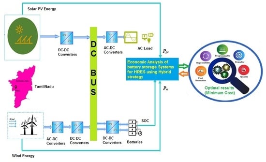
In this section, the economic analysis of the HRES system without and with energy storage is considered. The proposed technique is implemented in the MATLAB/Simulink platform. In order to meet the load demand of the system, PV, WT and battery have been utilized. HOMER is a free software application developed by the National Renewable Energy Laboratory in the United States. This software application is used to design and evaluate technically and financially the options for the off-grid and on-grid power systems for remote, stand-alone and distributed generation applications. It allows considering a large number of technological options to account for energy resource availability and other variables.

Here, two case studies are considered and discussed as follows:

Case Study A: Cost worked out for the interruption period without using energy storage.

Case Study B: Cost worked out using proposed technique for the interruption period with energy storage.

7.1. Case Study A

The existing 22 kV Vagarai feeder consists of one standalone 1.5 MW wind turbine (W₁), one 1.5 MW wind turbine (W₂-_PV) combined in a hybrid system with a 0.300 MW solar PV system and one standalone 2.8 MW wind turbine (W₃). In this case, study A, the cost analysis for the interruption period without using energy storage has been analyzed. Here, there is no generation during load curtailment and interruption periods of the system due to non-availability of battery storage. The results of case study A mainly show the impacts of higher load curtailment i.e., fault trip, main supply failure, shutdowns, etc.

Table 1. Quantum of energy really sold to the TANTRANSCO grid in KWHr during the year 2018 and the realization of actual cost of electricity ($/month).

Month	EW1	$-CW1	EW2 PV	$-CW2 PV	EW3	$-CW3	Export in KWHr	Total Cost ($)
January 2018	30,740	1476	152,380	7314	103,680	4977	286,800	13,766
February 2018	129,800	6230	154,180	7401	282,280	13,549	566,260	27,180
March 2018	26,400	1267	28,780	1381	50,480	2423	105,660	5072
April 2018	102,040	4898	113,080	5428	205,920	9884	421,040	20,210
May 2018	243,300	11,678	278,160	13,352	512,240	24,588	1,033,700	49,618
June 2018	605,760	29,076	592,980	28,463	1,490,320	71,535	2,689,060	129,075
July 2018	768,120	36,870	867,960	41,662	1,734,640	83,263	3,370,720	161,795
August 2018	676,560	32,475	686,100	32,933	1,341,680	64,401	2,704,340	129,808
September 2018	185,460	8902	188,400	9043	359,920	17,276	733,780	35,221
October 2018	53,240	2556	64,820	3111	100,240	4812	218,300	10,478
November 2018	77,260	3708	92,480	4439	151,800	7286	321,540	15,434
December 2018	117,700	5650	142,880	6858	236,920	11,372	497,500	23,880

lists the amount of energy really sold to the TANTRANSCO grid in KWHr and the actual cost of the electricity ($/month).

The quantum of the energy really purchased from the TANTRANSCO grid in KWHr and the actual cost paid for the electricity ($/month) is derived in

Table 2. Quantum of energy really purchased by the TANTRANSCO grid in KWHr and actual cost paid towards the electricity ($/month).

Month	IW1	$-CW1	IW2 PV	$-CW2 PV	IW3	$-CW3	Import (KWHr)	Total Cost ($)
January 2018	780	25.16	1040	49.92	720	38.88	2540	126.24
February 2018	640	22.86	860	41.28	960	51.84	2460	123.84
March 2018	460	14.84	540	25.92	560	30.24	1560	78.24
April 2018	1540	51.33	1560	74.88	1760	95.04	4860	243.84
May 2018	1540	49.68	920	44.16	1240	66.96	3700	185.04
June 2018	480	16.00	180	8.64	200	10.80	860	42.48
July 2018	580	18.71	300	14.40	280	15.12	1160	57.36
August 2018	120	3.87	40	1.92	80	4.32	240	12.00
September 2018	860	28.67	1560	74.88	1400	75.60	3820	191.76
October 2018	1240	40.00	2120	101.76	1920	103.68	5280	264.96
November 2018	1140	38.00	1780	85.44	1400	75.60	4320	215.76
December 2018	1420	45.81	1520	72.96	1440	77.76	4380	218.88

. The MATLAB/Simulation proves the generation cost is optimum after consideringthe sale of excess stored power. The total price ($/month) of electricity sold to grid monthly is denoted as I_{Import−month}.

The export of energy from the wind turbine (W₁) is denoted as E_W1, the export of energy from wind turbine (W₂) plus solar Photo Voltaic (PV) is denoted as (E_W2-PV) and the export of energy from the wind turbine (W₃) is denoted as E_W3 (per unit of power purchased from TANTRANSCO in INR is 3.30 [$ 0.48] for the W1 and W₂ plus PV solar hybrid system and INR 3.70 for W₃ [1 INR = $0.015]. C_W1 is the cost of the sale of power to grid due to the standalone 1.5 MW wind turbine. C_W2 is the cost of the sale of power to the grid due to the hybrid 1.5 MW wind turbine combined with the 0.300 MW solar PV systems and C_W3 is the cost of the sale of power to the grid due to the standalone 2.8 MW wind turbine. The import of energy from the wind turbine (W₁) is denoted as I_W1, The export of energy from the wind turbine (W₂) plus solar PV systemis denoted as I_{W2 PV} and the export of energy from the wind turbine (W₃) is denoted as I_W3 and per unit of power purchased from TANTRANSCO in INR is 3.30 [$0.48] for W₁ and W₂ plus solar PV hybrid system; and INR 3.70 is for W₃ [1 INR = $0.015]. Similarly, the import of energy for the wind turbine (W₁) is denote as I_W1, the import of energy for the wind turbine (W₂) plus solar PV systemis denoted as I_{W2 PV} and the import of energy for the wind turbine (W₃) is denoted as I_W3. Here, the export of energy from wind turbine (W₁) is denoted as E_W1 in column (2); export of energy from wind turbine (W₂) plus solar PV is denoted as E_{W2 PV} in column (3); and export of energy from wind turbine (W₃) is denoted as E_W3.The amountof energy really purchased by the grid through 22 kV feeders in the 110/22 kV Vagarai SS is tabulated in Table 2.

The actual current flown at 01.00 hon 19 July 2018 in all segments like 22 kV side, LV 1, LV2, Bus 1 and Bus 2; 110 kV side, GC and 110 kV Udumalpet/Renganathapuram in the switch yard is shown in Figure 7.

The hourly readings of the five 22 kV feeders in the 110/22 kV Vagarai substation and the L.V 1 and L.V 2 of the power transformers1 and 2 on 19 July 2018 are tabulated in

Table 3. Readings of all the 22 kV feeders including the hybrid generation regen feeder in the 110/22 kV Vagarai SS on 19 July 2018.

Date	Hybrid		22 Industrial		Rural		Rural		Industrial
19 July 2018	Regen Feeder		Agen Vijay		Appanuthu		VepanValasu		Mill
Time	Current (A)	MW	A	MW	A	MW	A	MW	A	MW
1.00 a.m.	−160	−5.5	30	1.0	30	1.0	65	2.2	10	0.3
2.00 a.m.	−155	−5.3	30	1.0	30	1.0	65	2.2	10	0.3
3.00 a.m.	−160	−5.5	30	1.0	25	0.9	70	2.4	10	0.3
4.00 a.m.	−160	−5.5	25	0.9	25	0.9	70	2.4	10	0.3
5.00 a.m.	−160	−5.5	30	1.0	30	1.0	70	2.4	10	0.3
6.00 a.m.	−160	−5.5	30	1.0	35	1.2	80	2.7	10	0.3
7.00 a.m.	−150	−5.1	30	1.0	35	1.2	100	3.4	50	1.7
8.00 a.m.	−160	−5.5	30	1.0	40	1.4	110	3.8	55	1.9
9.00 a.m.	−150	−5.1	25	0.9	35	1.2	100	3.4	65	2.2
10.00 a.m.	−165	−5.7	25	0.9	30	1.0	95	3.3	65	2.2
11.00 a.m.	−140	−4.8	25	0.9	25	0.9	85	2.9	65	2.2
12.00 Noon	−135	−4.6	30	1.0	30	1.0	75	2.6	65	2.2
01.00 p.m.	−130	−4.5	30	1.0	25	0.9	80	2.7	60	2.1
02.00 p.m.	−130	−4.5	30	1.0	30	1.0	80	2.7	60	2.1
03.00 p.m.	−125	−4.3	30	1.0	30	1.0	80	2.7	55	1.9
04.00 p.m.	−125	−4.3	35	1.2	30	1.0	85	2.9	60	2.1
05.00 p.m.	−160	−5.5	30	1.0	30	1.0	85	2.9	60	2.1
06.00 p.m.	−170	−5.8	30	1.0	35	1.2	90	3.1	60	2.1
07.00 p.m.	−120	−4.1	30	1.0	35	1.2	75	2.6	60	2.1
08.00 p.m.	−165	−5.7	30	1.0	35	1.2	75	2.6	60	2.1
09.00 p.m.	−140	−4.8	30	1.0	30	1.0	80	2.7	55	1.9
10.00 p.m.	−130	−4.5	30	1.0	30	1.0	75	2.6	55	1.9
11.00 p.m.	−130	−4.5	30	1.0	30	1.0	75	2.6	55	1.9
12.00 Night	−150	−5.1	30	1.0	30	1.0	70	2.4	55	1.9
	←------------------22 kV Bus-2------------------→						←-------------------22 kV Bus-1-------------------→

and

Table 4. Readings of the 22 kV regen feeder, LV1 and LV2 of power transformers 1 and 2, respectively in the 110/22 kV Vagarai SS on 19 July 2018.

Date	Hybrid		Power Tr. 2		Power Tr. l
19 July 2018	Regen Feeder		L.V 2		L.V 1
Time	Current (A)	MW	A	MW	A	MW
1.00 a.m.	−160	−5.5	−100	−3.42	75	2.57
2.00 a.m.	−155	−5.3	−95	−3.25	75	2.57
3.00 a.m.	−160	−5.5	−105	−3.60	80	2.74
4.00 a.m.	−160	−5.5	−110	−3.77	80	2.74
5.00 a.m.	−160	−5.5	−100	−3.42	80	2.74
6.00 a.m.	−160	−5.5	−95	−3.25	90	3.08
7.00 a.m.	−150	−5.1	−85	−2.91	150	5.14
8.00 a.m.	−160	−5.5	−90	−3.08	165	5.65
9.00 a.m.	−150	−5.1	−90	−3.08	165	5.65
10.00 a.m.	−165	−5.7	−110	−3.77	160	5.48
11.00 a.m.	−140	−4.8	−90	−3.08	150	5.14
12.00 Noon	−135	−4.6	−75	−2.57	140	4.79
01.00 p.m.	−130	−4.5	140	4.79	140	4.79
02.00 p.m.	−130	−4.5	140	4.79	140	4.79
03.00 p.m.	−125	−4.3	135	4.62	135	4.62
04.00 p.m.	−125	−4.3	145	4.97	145	4.97
05.00 p.m.	−160	−5.5	145	4.97	145	4.97
06.00 p.m.	−170	−5.8	150	5.14	150	5.14
07.00 p.m.	−120	−4.1	135	4.62	135	4.62
08.00 p.m.	−165	−5.7	100	3.42	135	4.62
09.00 p.m.	−140	−4.8	135	4.62	135	4.62
10.00 p.m.	−130	−4.5	130	4.45	130	4.62
11.00 p.m.	−130	−4.5	130	4.45	130	4.62
12.00 Night	−150	−5.1	135	4.62	135	4.62
	←---------22 kV Bus-2 ----------→				←-------22 kV Bus-1-------→

.

The 22 kV Bus 2 is connected with three 22 kV feeders, namely (1) Hybrid Generation Regen feeder, (2) Agen Vijay feeder and (3) Appanuthu feeder; whereas the 22 kV Bus 1 is connected with two 22 kV feeders, namely (4) VepanValasu feeder and (5) Mill feeder in the 110/22 kV Vagarai substation.

From Figure 7 and Table 3, it is seen that the required load was only 60 Amps (30 Amps each for the 22 kV Appanuthu and Agen Vijay feeders) on 22 kV Bus 2 and 75 Amps (10 Amps for 22 kV Mill feeder and 65 Amps for the 22 kV VepanValasu feeder).As the Bus coupler switch No. 12 was kept in an open condition, at 01.00 hon 19 July 2018, the power for an amount of 2.57 MW (75 Amps) out of 5.5 MW (160 Amps) from the hybrid feeder was stepped up to 110 kV by the power transformer (Pr. Tr)-2. And stepped down to 22 kV voltage level by power transformer (Pr. Tr)-1, (or, say from LV-2-Pr.Tr.2–Pr.Tr.1-LV-1) from the balance power of the 22 kV regen feeder, which is kept at 22 kV Bus-2.

Anamount of current of 100 Amps at the 22 kV side got transformed through the power transformer, as 20 Amps at the 110 kV side; and only an amount of 15 Amps at 110 kV equivalent to 5 Amps for the 22 kV side required for Bus 1. The balance amountof 5 Amps would flow to the 110 kV GC and finally be exported through 110 kV Udumalpet/Ranganathapuram feeders. Or, one can say that the required load demand for the 22 kV Veppen Valasu and 22 kV turbinefeeders was only 75 Amps @ 01.00 h, and the balance 25 Amps was fed into the power transformer 1 and stepped up to110 kV.

The actual current flown on all the 22 kV feeders in the 22 kV side in both the 22 kV Bus 1 and Bus 2 are given in Table 4 and Figure 7. At 01.00 h, the demand of the 22 kV Agen Vijay and Appanuthu feeders was 30 Amps each, whereas the hybrid generation of the regen feeder was 160 Amps.

Similarly, duringeach hour of 19 July 2018, the actual incoming generation from the hybrid regen feeder and the load demand of the remainingfour22 kV feeders and power flow to/from the 110 kV GC are recorded and charted in Table 3.

The time vs. current (in Amps) graph is given in Figure 8. From the graph, it is understood that the wind generation alone on the 22 kV hybrid feeder balanced the entire load of four 22 kV feeders. The unutilized amount of energy had been exported through the 110 kV Udumalpet/Ranganathapuram feeders from 01.00 a.m. to 06.00 a.m. on 19 July 2018.

As the load increased during the day hours and as the hybrid generation could not cater to the load, 110 kV GC imported power through the 110 kV Udumalpet/Ranganathapuram feeders from 7.00 a.m. onwards. If the 22 kV regen feeder is kept connected only with the solar generation, then there would not be any green energy from the wind and it would not fulfil the requirement at least up to some early hours of the day. In addition, if an energy storage system were implemented in the HRES, it would be more economical and beneficial and facilitate the generation of green energy even during predictable interruptions and curtailment periods also using the interconnectivity of the same grid.

The following

Table 5. Summary of all interruptions like fault trip, 110 kV main supply failure, load shedding, line clear, hand trip, break down and shut down in 110 kV Vagarai SS during the year of 2018.

Sl. No	Description	No. of Tripping	Duration of Interruptions
	Group 1:
a	Fault Trip	37	05 H 16 Min
b	Load Shedding	1	00 H 10 Min
c	Hand Trip	10	13 H 05 Min
d	Main 110 kV Supply failure	45	09 H 26 Min
	Group 2:
e	Total Shut down	9	65 H 35 Min
f	Line Clear	4	09 H 40 Min
g	Break Down of other feeders	11	109 H 15 Min
	Total	117	212 H 27 Min

is a summary of various interruptions occurred in the 110 kV Vagarai SS during the year of 2018.

From the table, it is understood that seven various types of generation interruption have occurredfor a total of 212 hours and 27 min during the year 2018. The different types of interruptions are described as fault trip, (b) load shedding, (c) hand trip, (d) main 110 kV supply failure, (e) total shut down (f) line clear and (g) breakdown of other feeders and equipment.Asummary of all month wiseinterruptions during the year of 2018 in the 110/22 kV Vagarai SS is presented in

Table 6. Summary showing all interruptions month wise during the year of 2018.

Total Interruption
Month	Hours	Min	Month	Hours	Min
January 2018	0	0.00	July 2018	14	11.00
February 2018	7	46.00	August 2018	81	9.00
March 2018	0	20.00	September 2018	55	17.00
April 2018	1	41.00	October 2018	10	40.00
May 2018	8	15.00	November 2018	14	46.00
June 2018	11	6.00	December 2018	7	16.00
Total	208 H plus 267 min = 208 + 4 H 27 Min, or say, 212 H 27 Min.

. All the interruptions can be grouped into two segments, some interruptions were predictable, and others were not predictable.

7.1.1. Interruptions That Would Not Be Predictable and Can Occur Suddenly

Interruptions like (a) fault trip, (b) load shedding (c) hand trip and (d) main 110 kV supply failure are categorized in this group. These interruptions could not be predicted. However, if a proper energy storage system is available; the energy can be stored by diverting the output through the breaker to the energy storage system. The number of occurrences of said unpredictable interruptions was 93 in the year 2018 but the total duration of the interruptions is only 27 h and 57 min, as given in

Table 7. Summary of unpredictable interruptions during the year 2018 in the 110 kV Vagarai SS.

Sl. No	Description	No. of Tripping	Duration of Interruptions
a	Fault Trip	37	05 h 16 min
b	Load Shedding	1	00 h 10 min
c	Hand Trip	10	13 h 05 min
d	Main 110 kV Supply failure	45	09 h 26 min
	Total	93	27 h 57 min

.

7.1.2. Interruptions That Are Predictable and Carried Out with Prior Intimation

Interruptions like (e) total shut down, (f) line clear and (g) proposed break down (BD) of other feeders and equipment are categorized in this group. The occurrence of the predictable interruptions during the year 2018, in the 110/22 kV Vagarai SS was 24 in number, but the duration was 184 h 30 min, as tabulated in

Table 8. Summary of predictable interruptions during the year 2018 in the 110 kV Vagarai SS.

Sl. No	Description	No. of Tripping	Duration of Interruptions
e	Total Shutdown	9	65 h 35 min
f	Line Clear	4	09 h 40 min
g	Breakdown of other feeders	11	109 h 15 min
	Total	24	184 h 30 min

.

These interruptions are normally taken intentionally for maintenance of equipment in the yard of the substation, it can be predictable, and in fact, the details of the interruptions would be conveyed over phone before being carried out. The duration of the interruptions isvery largeand the green power from the renewable energy sources can be stored; if a proper energy system is incorporated. As there is an alternative supply available for running the wind turbines, it can be possible to harness the green energy and store it in the energy storage system to be sold to the grid in the future.

7.2. Case Study B

In the case study B, the cost analysis for the interruption period using the proposed technique with energy storage has been analyzed. Here, the loss of the production of the green energy during grid interruptions and wind curtailment of the system are minimized because of the presence of battery storage using the proposed technique. Consequently, the proposed system gives lower cost with an optimal solution. The power flow in the HRES system using battery storage is analyzed forone day and one year. The variation of load per day and for a year is depicted in Figure 9.

Figure 9a the depicts how with the proposed technique the load demand is calculated during the time period of 24 h and Figure 9b illustrates the monthly load demand of the proposed technique. From Figure 9a, it is observed that the maximum hourly load demand of 5.9 MW is reached in the time intervals of 5 to 10 h. Likewise from Figure 9b, the maximum monthly load demand 1.39 × 10⁴ KW is reached during the time period of 10 to 12 h.

The graphs of irradiance and wind speed for a 24 h. period are plotted in Figure 10. From Figure 10a, it is observed that the irradiance of the system is a maximum of 1000 W/m² during the time-period of 10 to 15 h. The maximum wind speed 12 m/s is predicted at the time moment of 5 to 15 h. in Figure 10b.

Figure 11 shows the comparison analysis of power generated using energy storage, HOMER and the proposed technique for one day. Figure 11a depicts the graph of power versus time using the energy storage system. It is observed from Figure 11a, that by using the energy storage the maximum power 0.049 MW is generated in a period of 2 to 7 h. Figure 11b depicts the power generated using HOMER. By utilizing HOMER, the maximum power 0.047 MW is produced during the time interval of 20 to 25 h. Figure 11c shows the power generated using proposed technique. The maximum power generated using proposed technique is 0.05 MW at the time duration of 3 to 5 h.

Figure 12 shows the comparison analysis of power generated using energy storage, HOMER and proposed technique for one year. Figure 12a depicts agraph of power versus time using energy storage system. It is observed from the Figure 12a, which by using the energy storage the maximum power 1 MW is generated at the time period of 2 to 7 h. Figure 12b depicts the power generated using HOMER. By utilizing HOMER, the maximum power 1.3 MW is produced during the time interval of 2 to 4 h.

Figure 13 shows the individual generated power analysis using ESS, Without ESS, HOMER and Proposed for one day. Figure 13a shows the individual generated power using ESS. Figure 13a analyzes the PV, WT1, WT2 and WT3 generated power during the time period of 24 h. As seen from Figure 13a, the power generated by PV, WT1, WT2 and WT3 reaches the peak of 5.7 MW during the time instant of 5 to 10 h. Figure 13b shows the individual generated power without considering the ESS. From Figure 13b, it is observed that the power generated is in the maximum range of 5.75 MW at the time interval of 5 to 10 h. Figure 13c explains the individual generated power using HOMER. It is observed from the figure that the power generation is maximum 5.8 MW at the time duration of 5 to 10 h. Figure 13d delineates the individual generated power using the proposed technique. From Figure 13d, it is seen that the maximum power 5.9 MW is generated during the time interval of 5 to 10 h.

Figure 14 shows the individual generated power analysis using ESS, without ESS, HOMER and the proposed technique for one year. Figure 14a shows the individual generated power using ESS. Figure 14a analyzes the PV, WT1, WT2 and WT3 generated power during the time period of 24 h. As seen from Figure 14a, the power generated by PV, WT1, WT2 and WT3 reaches a peak of 160 MW during the time period of 6 to 8 h. Figure 14b shows the individual generated power without considering the BESS. From Figure 14b, it is observed that the power generated is in the maximum range of 155 MW during the time interval of 6 to 8 h. Figure 14c explains the individual generated power using HOMER. It is observed from the figure that the power generation is maximum 160 at the time periodof 6 to 8 h. Figure 14d delineates the individual generated power using proposed technique. From the Figure 14d, the maximum power 170 MW is generated during the time interval from 6 to 8 h.

Figure 15 shows the investigation of fitness graph for one day. It depicts the fitness comparison for one day. As seen from the figure, the base method solution converges after an iteration count of 32. The HOMER fitness solution converges at the 38^th iteration and the proposed technique gives the solution faster than the other techniques.

Figure 16 shows the investigation of cost for one day and one year. Figure 16a depicts the graph of cost versus time. The cost of the proposed technique is more optimal for one day than the other techniques such as without ESS, Base and HOMER. Figure 16b depicts the graph of cost versus time. The cost of the proposed technique is more optimal for one year than the other techniques such as without ESS, Base and HOMER.

Figure 17 shows the investigation of fitness graph for one year.

As seen from the Figure 17, the base method solution converges after 49 iterations. The HOMER fitness solution converges at the 41^st iteration and the proposed technique gives the solution faster than the other techniques.

8. Conclusions

The present study has been carried out for the optimization of hybrid renewable energy systems (HRES), where WT and PV function as generation systems and battery banks for storage as well as a backup system usingthe RBFNOEHO technique. Here, an existing hybrid system with both solar and wind generation combined and formed as 22 kV feeder and fed into the 110/22 kV Vagarai substation in the Palani Division in the Dindigul Circle of TANGEDCO in the State of Tamil Nadu of Indiahas been chosen for study purposes. The economic analysis of battery storage for the HRES system using the proposed hybrid technique is discussed. By utilizing the proposed hybrid technique, the load demand is predicted and the total cost of the system is minimized. Here, two case studies are analyzed. First, the cost is worked out for interruption periods without using energy storage and in the second, the cost is worked out using the proposed technique for the interruption periods with energy storage. According to the results, it is concluded that the hybrid systems including WT and PV with battery backup are less costly compared to the other systems.

References

1. Dincer, I. Renewable energy and sustainable development: A crucial review. Renew. Sustain. Energy Rev. 2000, 4, 157–175. [Google Scholar] [CrossRef]
2. Padmanathan, K.; Govindarajan, U.; Ramachandaramurthy, V.K.; Rajagopalan, A.; Pachaivannan, N.; Sowmmiya, U.; Padmanaban, S.; Holm-Nielsen, J.B.; Xavier, S.; Periasamy, S.K. A Sociocultural Study on Solar Photovoltaic Energy System in India: Stratification and Policy Implication. J. Clean. Prod. 2019, 216, 461–481. [Google Scholar] [CrossRef]
3. Padmanathan, K.; Govindarajan, U.; Ramachandaramurthy, V.K.; Sudar Oli Selvi, T. Multiple Criteria Decision Making (MCDM) Based Economic Analysis of Solar PV System with Respect to Performance Investigation for Indian Market. Sustainability 2017, 9, 820. [Google Scholar] [CrossRef]
4. Padmanathan, K.; Uma, G.; Ramachandaramurthy, V.K.; Sudar Oli Selvi, T.; Baskaran, J. Integrating solar photovoltaic energy conversion systems into industrial and commercial electrical energy utilization—A survey. J. Ind. Inf. Integr. 2018, 10, 39–54. [Google Scholar]
5. Owusu, P.; Asumadu-Sarkodie, S. A review of renewable energy sources, sustainability issues and climate change mitigation. Cogent Eng. 2016, 3, 1167990. [Google Scholar] [CrossRef]
6. Omer, A. Energy, environment and sustainable development. Renew. Sustain. Energy Rev. 2008, 12, 2265–2300. [Google Scholar] [CrossRef]
7. Panwar, N.; Kaushik, S.; Kothari, S. Role of renewable energy sources in environmental protection: A review. Renew. Sustain. Energy Rev. 2011, 15, 1513–1524. [Google Scholar] [CrossRef]
8. Heard, B.; Brook, B.; Wigley, T.; Bradshaw, C. Burden of proof: A comprehensive review of the feasibility of 100% renewable-electricity systems. Renew. Sustain. Energy Rev. 2017, 76, 1122–1133. [Google Scholar] [CrossRef]
9. Liang, X. Emerging Power Quality Challenges Due to Integration of Renewable Energy Sources. IEEE Trans. Ind. Appl. 2017, 53, 855–866. [Google Scholar] [CrossRef]
10. Blaabjerg, F.; Teodorescu, R.; Liserre, M.; Timbus, A. Overview of Control and Grid Synchronization for Distributed Power Generation Systems. IEEE Trans. Ind. Electron. 2006, 53, 1398–1409. [Google Scholar] [CrossRef] [Green Version]
11. Divya, K.; Ostergaard, J. Battery energy storage technology for power systems—An overview. Electr. Power Syst. Res. 2009, 79, 511–520. [Google Scholar] [CrossRef]
12. Zhao, H.; Wu, Q.; Hu, S.; Xu, H.; Rasmussen, C. Review of energy storage system for wind power integration support. Appl. Energy 2015, 137, 545–553. [Google Scholar] [CrossRef]
13. Choi, J.; Heo, S.; Kim, M. Hybrid operation strategy of wind energy storage system for power grid frequency regulation. IET Gener. Transm. Distrib. 2016, 10, 736–749. [Google Scholar] [CrossRef]
14. Ibrahim, H.; Ilinca, A.; Perron, J. Energy storage systems—Characteristics and comparisons. Renew. Sustain. Energy Rev. 2008, 12, 1221–1250. [Google Scholar] [CrossRef]
15. Sedghi, M.; Ahmadian, A.; Aliakbar-Golkar, M. Optimal Storage Planning in Active Distribution Network Considering Uncertainty of Wind Power Distributed Generation. IEEE Trans. Power Syst. 2016, 31, 304–316. [Google Scholar] [CrossRef]
16. Karunakaran, V.; Uma, G. Optimal Power Flow control of Hybrid renewable energy system with energy storage: A WOANN strategy. J. Renew. Sustain. Energy 2019, 11, 015501. [Google Scholar] [CrossRef]
17. Yin, P.Y. A fast scheme for multilevel thresholding using genetic algorithms. Signal Process. 1999, 72, 85–95. [Google Scholar] [CrossRef]
18. Hammouche, K.; Diaf, M.; Siarry, P. A multilevel automatic thresholding method based on a genetic algorithm for fast image segmentation. Comput. Vis. Image Underst. 2008, 109, 163–175. [Google Scholar] [CrossRef]
19. Zhang, J.; Li, H.; Tang, Z.; Lu, Q.; Zheng, X.; Zhou, J. An improved quantum inspired genetic algorithm for image multilevel thresolding segmentations. Math. Probl. Eng. 2014, 112, 1–12. [Google Scholar] [CrossRef]
20. Simon, D. Biogeography based optimization. IEEE Trans. Evol. Comput. 2008, 12, 702–713. [Google Scholar] [CrossRef]
21. Yin, P.Y. Multilevel minimum cross entropy threshold selection based on Particle swarm Optimization Algorithm. Appl. Math. Comput. 2007, 184, 503–513. [Google Scholar]
22. Kennady, J.; Eberhart, R.C. Particle swarm Optimization. In Proceedings of the IEEE International Conference of Neural Network, Perth, Australia, 27 November–1 December 1995; Volume 4, pp. 1942–1948. [Google Scholar]
23. Akay, B. A study on Particle swarm Optimization and artificial bee colony algorithms for multilevel thresholding. Appl. Soft Comput. 2013, 13, 3066–3091. [Google Scholar] [CrossRef]
24. Gandomi, A.H.; yang, X.S.; Talatahari, S.; Deb, S. Coupled eagle strategy and differential evaluation for unconstrained global optimization. Comput. Math. Appl. 2012, 63, 191–200. [Google Scholar] [CrossRef]
25. Sathya, P.D.; Kayalvizhi, R. Optimum multilevel image thresholding based on Tsallis entropy method with bacterial foraging algorithm. Int. J. Comput. Sci. 2010, 7, 336–343. [Google Scholar]
26. Tao, W.; Jin, H.; Liu, L. Object segmentation using ant colony optimization algorithm and fuzzy entropy. Pattern Recognit. Lett. 2007, 28, 788–796. [Google Scholar] [CrossRef]
27. Agarwal, S.; Panda, R.; Bhuyan, S.; Panigrahi, B.K. Tsallis entropy based optimal multilevel thresholding using Cuckoo Search algorithm. Swarm Evol. Comput. 2013, 11, 16–30. [Google Scholar] [CrossRef]
28. Horng, M.H. Multilevel minimum cross entropy thresehold selection based on the honey bee mating optimization. Expert Syst. Appl. 2010, 37, 4580–4592. [Google Scholar] [CrossRef]
29. Yang, X.S. A new metaheuristic bat-inspired algorithm. In Nature Inspired Cooperative Strategies for Optimization; Springer: Berlin, Germany, 2010; Volume 284, pp. 65–74. [Google Scholar]
30. Kim, S.; Lee, H.; Kim, H.; Jang, D.H.; Kim, H.J.; Hur, J.; Cho, Y.S.; Hur, K. Improvement in policy and proactive interconnection procedure for renewable energy expansion in South Korea. J. Renew. Sustain. Energy Rev. 2018, 98, 150–162. [Google Scholar] [CrossRef]
31. Chen, F.; Lu, S.M.; Tseng, K.T.; Lee, S.C.; Wang, E. Assessment of renewable energy reserves in Taiwan. Renew. Sustain. Energy Rev. 2010, 14, 2511–2528. [Google Scholar] [CrossRef]
32. Dai, J.; Yang, X.; Wen, L. Development of wind power industry in China: A comprehensive assessment. Renew. Sustain. Energy Rev. 2018, 97, 156–164. [Google Scholar] [CrossRef]
33. Liu, Y.; Zhang, J. Research on the effects of wind power grid to the distribution network of Henan province. AIP Conf. Proc. 2018, 1955, 030005. [Google Scholar] [CrossRef]
34. Islam, M.R.; Sarker, P.C.; Ghosh, S.K. Prospect and advancement of solar irrigation in Bangladesh: A review. Renew. Sustain. Energy Rev. 2017, 77, 406–422. [Google Scholar] [CrossRef]
35. Islam, M.R.; Islam, M.R.; Beg, M.R. Renewable energy sources and technologies practice in Bangladesh. Renew. Sustain. Energy Rev. 2008, 12, 299–343. [Google Scholar] [CrossRef]
36. Pham, B.; Shirzadi, A.; Tien Bui, D.; Prakash, I.; Dholakia, M. A hybrid machine learning ensemble approach based on a Radial Basis Function neural network and Rotation Forest for landslide susceptibility modeling: A case study in the Himalayan area, India. Int. J. Sediment Res. 2018, 33, 157–170. [Google Scholar] [CrossRef]
37. Chakraborty, F.; Roy, P.; Nandi, D. Oppositional elephant herding optimization with dynamic Cauchy mutation for multilevel image thresholding. Evol. Intell. 2019, 1–23. [Google Scholar] [CrossRef]
38. Murugaperumal, K.; Raj, P.A. Energy storage based MG connected system for optimal management of energy: An ANFMDA technique. Int. J. Hydrog. Energy 2019, 44, 7996–8010. [Google Scholar] [CrossRef]
39. World weather Home Page. Available online: https://www.worldweatheronline.com/lang/en-in/palani-weather-averages/tamil-nadu/in.aspx (accessed on 26 July 2019).
Figure 1. The average and maximum wind speed and wind gust over the years in Palani, India.
Energies 12 03047 g001
Figure 2. The average sun hours and sun days over the years in Palani, India.
Energies 12 03047 g002
Figure 3. Switchyard arrangement of the 22 KV hybrid feeder in the 110/22 KV Vagarai SS.
Energies 12 03047 g003
Figure 4. System configuration of the HRES system.
Energies 12 03047 g004
Figure 5. Process of economic analysis of the proposed system.
Energies 12 03047 g005
Figure 6. Flowchart of the proposed technique.
Energies 12 03047 g006
Figure 7. Actual flowchart of both the 110 kV and 22 kV sides @ 01.00 hour on 19 July 2018 in the 110 kV SS.
Energies 12 03047 g007
Figure 8. Time vs. current graph showing the actual current flowed with respect to hours of the day on each of the 22 kV feeders and LV1, LV2 and GC of the 110 Vagarai substation on 19 July 2018.
Energies 12 03047 g008
Figure 9. Demand versus time profile of the proposed technique for (a) one day (b) one year.
Energies 12 03047 g009
Figure 10. Analysis of (a) Irradiance (b) Wind Speed for one day.
Energies 12 03047 g010
Figure 11. Comparison analysis of the power generated using (a) With ESS (b) HOMER (c) Proposed technique for one day.
Energies 12 03047 g011
Figure 12. Comparison analysis of power generated using (a) With ESS (b) HOMER (c) Proposed technique for one year.
Energies 12 03047 g012
Figure 13. Individual Power analysis (a) With ESS (b) Without ESS (c) HOMER (d) Proposed technique for one day.
Energies 12 03047 g013
Figure 14. Individual power analysis: (a) With ESS (b) Without ESS (c) HOMER (d) Proposed technique for one year.
Energies 12 03047 g014
Figure 15. Investigation of Fitness comparison for one day.
Energies 12 03047 g015
Figure 16. Investigation of cost for (a) One day (b) One year.
Energies 12 03047 g016
Figure 17. Investigation of Fitness comparison for one year.
Energies 12 03047 g017