Reference and Limit Governors for Limit Protection of Turbofan Engines

Abstract

This paper proposes a novel architecture of limit protection including the references governors and limit governors and applies this architecture to limit protection in turbofan engines. References governors are designed as add-on schemes to a pre-stability engine control system that modifies reference commands to avoid constraints violation. Limit governors are proposed as an assistant part for references governors adjusting constraints to prevent references from stopping updates. The use of output admissible sets for a class of variable constraints is exploited to form invariant sets. Simulation results based on a turbofan engine model show that references governors with limit governors can effectively enforce the multiple constraints and provide enhanced engine thrust when steady violation occurs.

1. Introduction

The implementation of advanced control systems on aircraft turbofan engines requires the effective limit protection, which keeps the engine operating within its constraints [1]. These constraints prevent the engine components from risky operating conditions such as surge, stall and flame blowout avoidance, pressures and temperatures limits, over fan and core speeds, actuator magnitude and rate limits.

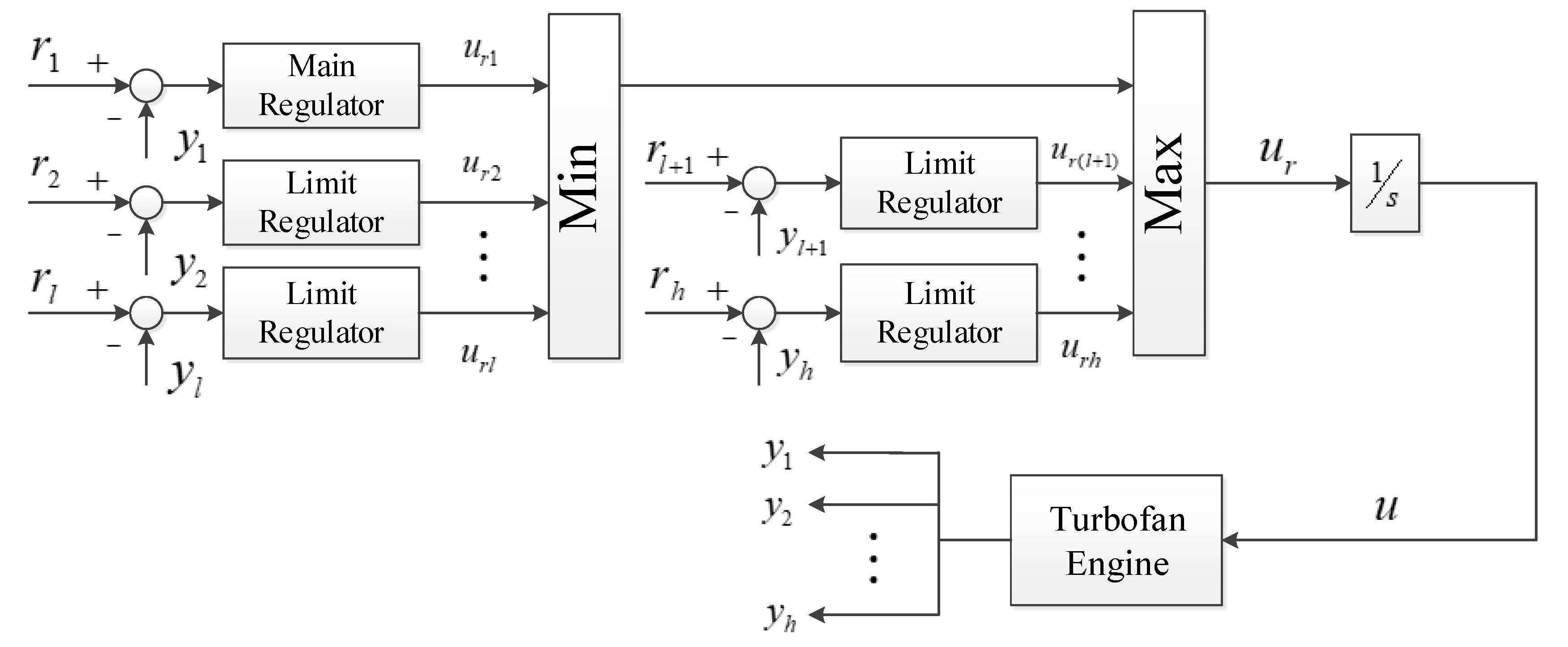
Turbofan engine control systems have incorporated methods to avoid these constraint violations. The conventional and widely used method to handle these constraints is using a Min–Max architecture as shown in Figure 1 [2]. The linear single-input main regulator is designed to drive the fan speed and several auxiliary linear regulators are used to maintain the limited variables. Main and auxiliary regulators are combined with a Min–Max selector that selects an auxiliary regulator when it is necessary to avoid a specific constraint violation. All regulators use fuel flow rate as the single control channel. The fuel flow rate applied to the integrator is selected according to the formula:

$$u_r=\underset{k\in H}{\max }\{\underset{j\in L}{\min \{u_{rj}\},u_{rk}}\}$$

(1)

where $L$ contains the indices of the regulators associated with the Min selector, $H$ contains the indices of the regulators with the max selector, $u_{rj}$ are the min-selected regulator outputs and $u_{rk}$ are the max-selected regulator outputs. In this paper, this approach will be considered as the traditional Min–Max (TMM) approach. Since it has been demonstrated that the TMM approach is inherently conservative and produces slower transient responses, the interest in developing methods to reduce the conservatism of the limit protection approach has been growing [3].

In recent decades, techniques have been developed to improve the TMM approach. In [3], conditional active limit regulators are added on the Min–Max architecture. Numerous candidates have also been applied to design the regulators for Min–Max architecture such as sliding mode control [4,5] and monotonic control [6]. However, a large number of technologies with limited protection functions that are not based on the Min–Max structure have been developed for aircraft engines. One of the existing approaches to handle constraints is the model predictive control (MPC) [7,8]. MPC will re-design the controller to achieve not only the limit protection function but also the main control tasks. Other approaches consider augmenting a well-designed controller with a constraint handling capability [9,10,11,12,13]. This kind of approach is attractive by preserving existing controllers that have well-designed control quality. The augmentation with barrier functions is an example of this kind of approach, and the reference governors are the same.

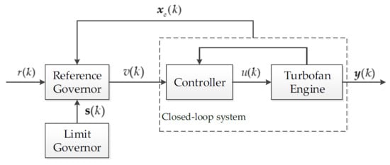
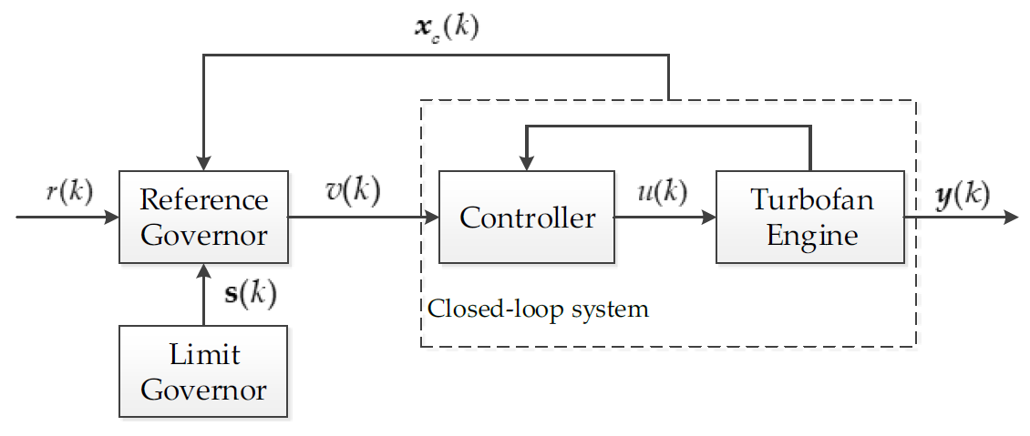
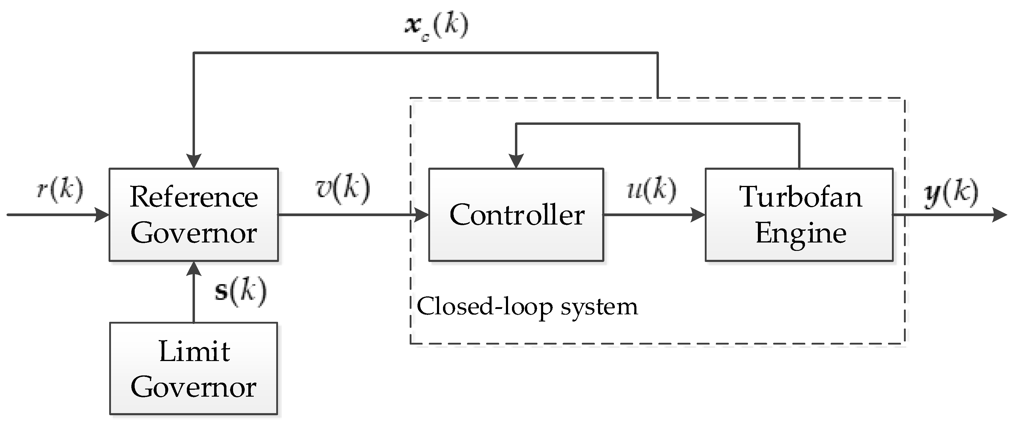
In this paper, we focus on the application of references governors (RGs) to limit protection in turbofan engines. RGs are an add-on scheme for enforcing closed-loop system constraints by predictively modifying the reference commands to the closed-loop system when necessary. While RGs have been researched for over twenty years and studies of applications cover many areas [14,15,16], there are still several challenges in applying RGs from the practical standpoint such as the infeasibility treatment [17]. When the online optimization problem does not admit a solution, the widely used strategy is to continue applying the previous reference. Nevertheless, this could result in the stop of updating reference and the tracking rate will slow down. More seriously, if the infeasibility occurs for a long time, the main tracking aim will not be achieved. The situation described above may occur for two reasons. One is enhanced engine thrust requirements make the engine operate beyond normal operational limits, which is called steady violation. The other is the RG designed has a constrained domain of attraction that is not large enough. When steady violation occurs, prioritized reference governors can enforce over-limit constraints as soft constraints in the order of their priority so that if all constraints cannot be strictly met, slight violation of the soft constraints will be permitted [18]. The extended command governors use more degrees of freedom to find feasible solutions through optimization, which expands constrained domains of attraction by adding optimization parameters and inevitably increases the computational cost of the optimization problem [19]. In this paper, a novel architecture containing RGs and limit governors (LGs) are proposed to enhance the engine thrust and expand the constrained domain of attraction, shown in Figure 2. In addition, the architecture proposed simplifies the structure and makes an improvement of transient performance compared to the TMM architecture. The main strategy is to avoid introducing as many optimization parameters as possible while expanding constrained domain of attraction. When the RG online optimization problem has no solution, the LG will slack the constraint values within a limit band according to the off-line designed constraint slack law. Due to the inherent risky nature of slacking constraints, it is important to design limit bands referring to risk management [20]. Based on the selected risk level, an operating limit band can be selected. Detailed design methods will not be considered in the article.

This paper is organized as follows. In Section 2, the design of the turbofan engine controller and the establishment of the prediction model are discussed. The design methods and details of RGs and LGs are discussed in Section 3, followed by the simulation results and discussion in Section 4. Conclusions are given in Section 5.

2. Turbofan Engine Control Method and Prediction Model

A modern twin-spool turbofan engine was studied in this paper. A high degree of confidence component level model of the turbofan engine has been achieved and details and details can be seen in [21,22]. The turbofan engine mainly consists of the following components: Inlet, fan, compressor, combustor, high pressure turbine (HPT), low pressure turbine (LPT), bypass and nozzle [23]. Each component was modeled by aerothermodynamics calculations and solving a set of balance equations. The engine design operation data and characteristic maps of rotating components were used to construct the turbofan engine nonlinear model. The nonlinear model of turbofan engine is given by:

$$\{\begin{array}{c}\dot{x}=f(x,u)\\ y=g(x,u)\end{array},$$

(2)

where $x\in R^n$ is the state vector, $u\in R$ is the input variable and $y\in R^p$ is the output vector.

The engine model was coded with the C language and packaged by the Dynamic Link Library (DLL) for simulation in a Matlab environment. This engine model has been also used in other closed-loop control research [24,25]. The detailed nonlinear model can calculate steady state data and response data at arbitrary operating point. The operating point is defined by altitude (ALT), Mach number (MN) and power lever angle (PLA). For given ALT, MN and PLA, there is a corresponding operating point described by an equilibrium point $(x_e,y_e)$ and a steady-state control $u_e$. The linear model at the operating point can be obtained by the hybrid fitting method, which combines partial perturbing and fitting methods [26]. The linear model is presented as:

$$\{\begin{array}{c}\Delta x(k+1)=A\Delta x(k)+B\Delta u(k)\\ \Delta y(k)=C\Delta x(k)+D\Delta u(k)\end{array}$$

(3)

where $A$, $B$, $C$ and $D$ are the system matrices with appropriate dimensions and $\Delta x=x-x_e$, $\Delta u=u-u_e$ and $\Delta y=y-y_e$.

2.1. Augment LQ Tracking Controllers for Discrete Systems

We considered the discrete linearized models for the engine. $\Delta x$, $\Delta u$ and $\Delta y$ are replaced by $x$, $u$ and $y$ for convenience in the subsequent article. The linear model is rewritten as:

$$\{\begin{array}{c}x(k+1)=Ax(k)+Bu(k)\\ y(k)=Cx(k)+Du(k)\end{array}$$

(4)

The $i\mathrm{th}$ output is:

$$y_i(k)=C_{i}x(k)+D_{i}u(k)$$

(5)

where $i=1,2,\dots ,p$, $C_i$ is the $i\mathrm{th}$ row of the matrix $C$ and $D_i$ is the $i\mathrm{th}$ element of the matrix $D$.

Considering the controller includes integral action $u_r(k)$:

$$u_r(k)=u(k+1)-u(k)$$

(6)

The state-space description is augmented:

$$\{\begin{array}{c}{x}_a(k+1)=A_a{x}_a(k)+B_a{u}_r(k)\\ y(k)=C_a{x}_a(k)+D_a{u}_r(k)\end{array}$$

(7)

where $u_r(k)\in R$ is the new input variable, the augmented state vector is defined as $x_a(k)={[x^{\mathrm{T}}(k)u^{\mathrm{T}}(k)]}^{\mathrm{T}}$ and the augmented matrices are defined as:

$$A_a=\left[\begin{array}{cc}A& B\\ \mathbf{0}& 1\end{array}\right],B_a=\left[\begin{array}{c}\mathbf{0}\\ 1\end{array}\right],C_a=[C\hspace{1em}D],D_a=\mathbf{0}.$$

(8)

For single input, $y_1$ is chosen as the main regulated output (typically fan speed), whose set-point is to be tracked with zero steady-state error. The other outputs $y_i$ ($i=2,3,\dots ,p$), (typically high-pressure turbine outlet temperature and low-pressure compressor outlet pressure [1]) are used as limited variables, which are discussed later in the paper. In this section, the main control objective was set-point tracking for main regulated output. Let $r\in R$, $u_s$, $x_s$ denote the tracking reference, control input and state as $k\to \infty$, respectively. Define an augmented steady state $x_{a,s}=\left[\begin{array}{c}{x}_s\\ u_s\end{array}\right]$ and $Z=\left[\begin{array}{cc}A-I& B\\ C_1& D_1\end{array}\right]$, the steady state value was calculated by:

$$x_{a,s}=Z^{-1}\left[\begin{array}{c}\mathbf{0}\\ r\end{array}\right]$$

(9)

Define the steady state deviation:

$$\mathbf{\Delta }{x}_a(k)={\left[\begin{array}{cc}\mathbf{\Delta }{x}^{\mathrm{T}}(k)& \Delta u^{\mathrm{T}}(k)\end{array}\right]}^{\mathrm{T}}={\left[\begin{array}{cc}{\left(x(k)-x_s\right)}^{\mathrm{T}}& {\left(u(k)-u_s\right)}^{\mathrm{T}}\end{array}\right]}^{\mathrm{T}},$$

(10)

then,

$$\{\begin{array}{c}\mathbf{\Delta }{x}_a(k+1)=A_a\mathbf{\Delta }{x}_a(k)+B_a{u}_r(k)\\ y_1(k)-r=C_{a,1}\mathbf{\Delta }{x}_a(k)\end{array}$$

(11)

where $C_{a,1}$ is the first row of $C_a$.

Given the system presented in (11), the optimal LQ controller was obtained by using the state-feedback gain $K_a$ that minimizes a performance index:

$$J=\frac{1}{2}{\displaystyle \sum _{k=0}^{\infty }\left[\mathbf{\Delta }{x}_a^{\mathrm{T}}(k)Q\mathbf{\Delta }{x}_a(k)+u_r^{\mathrm{T}}(k)R{u}_r(k)\right]},$$

(12)

where $Q$ is a symmetric positive semi-definite matrix and $R$ is a symmetric positive-definite matrix. The pairs $(A_a,B_a)$ and $(B_a,C_{a,1})$ were assumed to be controllable and observable respectively.

The optimal controller is given in the form of state feedback

$$u_r(k)=-K_a\mathbf{\Delta }{x}_a(k).$$

(13)

The feedback matrix $K_a$ is obtained by solving the Riccati equation.

$$A_a^{\mathrm{T}}P{A}_a-P-A_a^{\mathrm{T}}P{B}_a{(R+B_a^{\mathrm{T}}P{B}_a)}^{-1}{B}_a^{\mathrm{T}}P{A}_a=-Q.$$

(14)

Considering the difficulty of using steady state deviation $\mathbf{\Delta }{x}_a(k)$ to achieve feedback control, $\mathbf{\Delta }{x}_a(k)$ can be replaced by $x(k)$ and $r(k)-y_1(k)$. The replacement eliminates the calculation of tracking steady state $x_s$ and control input $u_s$ and introduces variables that are easier to obtain online. In addition, the system can realize tracking without steady-state error due to the tracking error is introduced into the state feedback controller.

Combined with Equations (4), (9), (10), (13), the following equations can be derived:

$$u_r(k)=-K_a\left[\begin{array}{c}x(k)\\ u(k)\end{array}\right]+K_a\left[\begin{array}{c}{x}_s\\ u_s\end{array}\right],$$

(15)

$$\left[\begin{array}{c}x(k)\\ u(k)\end{array}\right]=Z^{-1}\left[\begin{array}{c}x(k+1)-x(k)\\ y_1(k)\end{array}\right],$$

(16)

$$u_r(k)=-K_a{Z}^{-1}\left[\begin{array}{c}x(k+1)-x(k)\\ y_1(k)-r\end{array}\right].$$

(17)

Define $x_r(k)=x(k+1)-x(k)$, $\left[\begin{array}{cc}{K}_1& K_2\end{array}\right]=-K_a{Z}^{-1}$, where $K_1\in R^n$ and $K_2\in R$. In practical applications, $x(k+1)-x(k)$ can be approximately replaced by $x(k)-x(k-1)$ which means $x_r(k)=x(k)-x(k-1)$, thus:

$$u_r(k)=K_1{x}_r(k)+K_2(y_1(k)-r).$$

(18)

This approximation enables the integral action $u_r(k)$ can be calculated at the current sample time and the error of approximation can be ignored because of the extremely short sampling time and sufficiently slow rates of time variation in system states.

2.2. Modeling Methods of the Closed-Loop System

The RG in this paper is based on a linear discrete-time model of the engine. Based on Equation (5), the nominal controller can be rewritten as:

$$u_r(k)=K_1{x}_r(k)+K_2{C}_{1}x(k)+K_2{D}_{1}u(k)-K_{2}r,$$

(19)

With the LQ controller (19), the closed loop system prediction model becomes:

$$\{\begin{array}{c}{x}_c(k+1)=A_c{x}_c(k)+B_{c}v(k)\\ y(k)=C_c{x}_c(k)+D_{c}v(k)\end{array},$$

(20)

where $A_c=\left[\begin{array}{cc}A& \mathbf{0}\\ \mathbf{0}& A_a\end{array}\right]+\left[\begin{array}{c}B\\ B_a\end{array}\right]\left[\begin{array}{ccc}{K}_1& K_2{C}_1& K_2{D}_1\end{array}\right]$, $B_c=-K_2{\left[\begin{array}{cc}B& B_a\end{array}\right]}^{\mathrm{T}}$, $C_c=\left[\begin{array}{cc}\mathbf{0}& C_a\end{array}\right]+D_a\left[\begin{array}{ccc}{K}_1& K_2{C}_1& K_2{D}_1\end{array}\right]$ and $D_c=-K_2{D}_a$, $x_c(k)={\left[\begin{array}{cc}{x}_r(k)& x_a(k)\end{array}\right]}^{\mathrm{T}}$ denotes the states of the closed-loop system, $v(k)$ is the admissible reference command, which will be determined by a solution of the online optimization problem discussed in Section 3.

The system matrices play the important roles in the steady and transient performance of the closed-loop system prediction model. However, the system matrices in model (20) cannot accurately describe the steady and transient performance of the turbofan engine and the controller because of the nonlinearity of the combination of turbofan engines and controllers. In order to improve modeling accuracy of the closed-loop system, a fitting method is used to re-compute partial system matrices’ elements [27]. The fitting method generates the system matrices’ elements with the object function of least square errors between the closed-loop system and closed-loop system prediction model responses to step reference. In this paper, the matrix $A_c$ remains constant to ensure the stability of the prediction model and the matrix $D_c$ stays at $0$.

The procedure of the modeling method is summarized as follows.

(1)

Establish a linearized turbofan engine model at an equilibrium point by hybrid fitting method.

(2)

Design a nominal tracking controller at the same equilibrium point.

(3)

The initials matrices of the closed-loop system prediction model are given by substituting the controller into the linearized model.

(4)

The closed-loop system prediction model matrices are tuned to the outputs differences of the closed-loop system and closed-loop system prediction model at the equilibrium point by fitting method. In the end, the closed loop system prediction model is established as:

$$\{\begin{array}{c}{x}_c(k+1)=A_c{x}_c(k)+B_{rc}v(k)\\ y(k)=C_{rc}{x}_c(k)+D_{c}v(k)\end{array},$$

(21)

where matrices $B_{rc}$ and $C_{rc}$ are re-computed matrices.

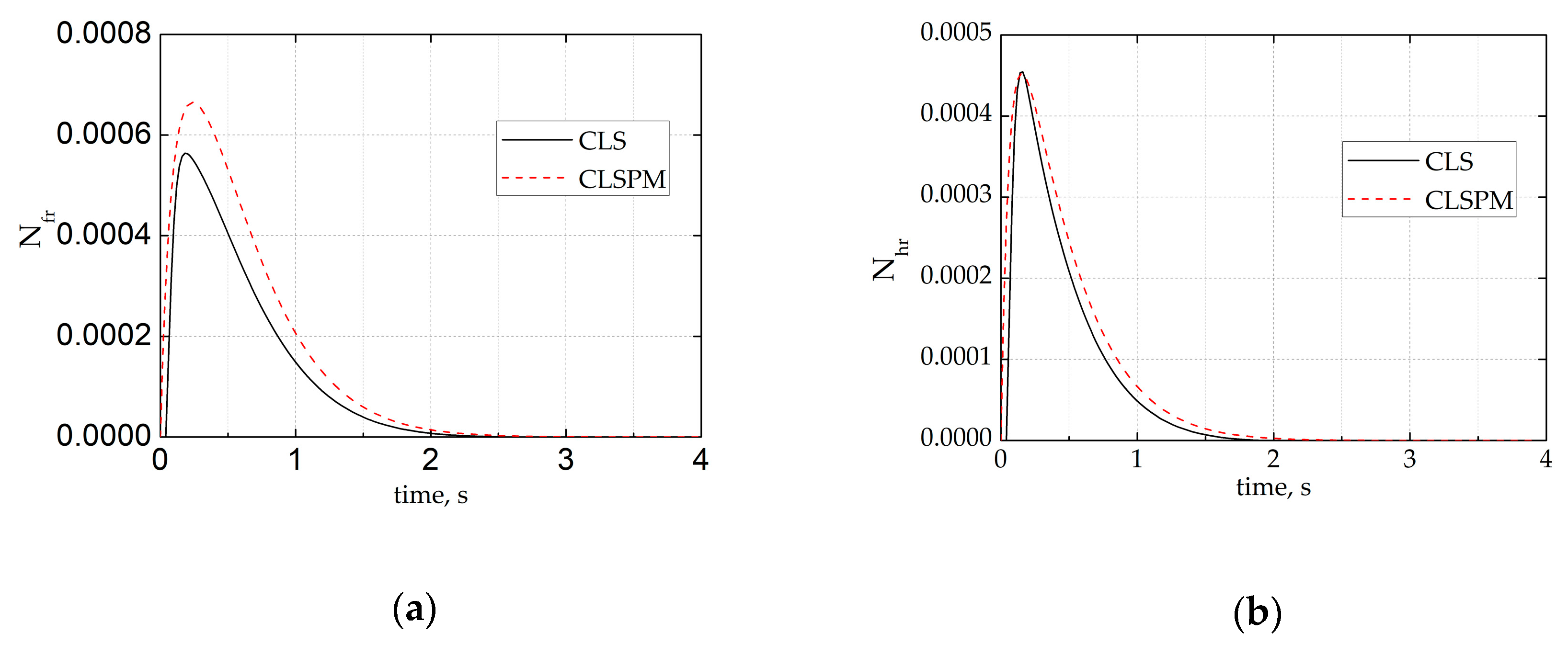
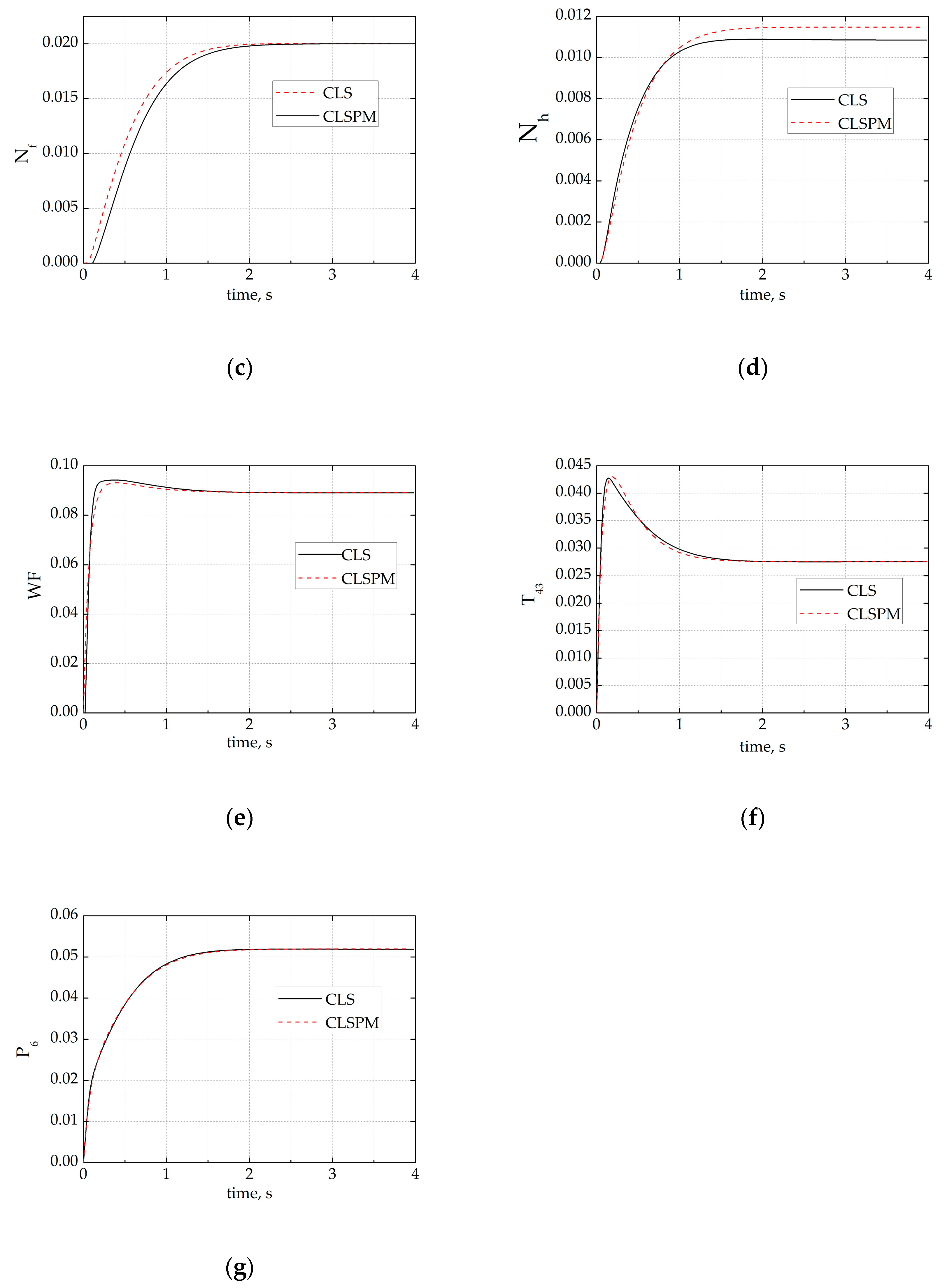
Figure 3 presents the response comparisons of the closed-loop system (CLS, black solid line), closed-loop system prediction model (CLSPM, red dash line) respectively under 2% step reference at the 75% fan speed at ground. The results show that the response of CLSPM could track the response of CLS.

3. Reference Governors with Limit Governors

3.1. Reference Governors

RGs are add-on predictive control schemes that enforce state and control constraints in discrete-time closed-loop systems. Unlike conventional MPC schemes, which enforce constraints and ensure system stability, RGs are used to augment systems with closed-loop controllers that may have been designed without taking constraints into account [28].

As the control input rate $u_r(k)$ is considered as a constraint, it is convenient to augment the control input rate $u_r(k)$ to outputs by Equation (18),

$$\{\begin{array}{c}{x}_c(k+1)=A_c{x}_c(k)+B_{rc}v(k)\\ y_c(k)=C_{arc}{x}_c(k)+D_{ac}v(k)\in Y\end{array},$$

(22)

where $C_{arc}=\left[\begin{array}{c}{C}_{rc}\\ K_1\hspace{1em}{K}_2{C}_1\hspace{1em}{K}_2{D}_1\end{array}\right]$, $D_{ac}=\left[\begin{array}{c}{D}_c\\ -K_2\end{array}\right]$ and $y_c=\left[\begin{array}{c}y\\ u_r\end{array}\right]$.

The classical reference governor is designed for a discrete-time linear system model of the form like model (22). The objective of RGs is to manage the applied command $v(k)$, which should be as close as possible to the desired reference $r$ and to guarantee that the system constraints $y_c(k)\in Y$, $Y=\{y_c|S{y}_c\le s\}$ is enforced. Some assumptions were made here:

Assumption 1.

All eigenvalues of $A_c$ were in the unit disk.

Assumption 2.

The pair $(C_{arc},A_c)$ was observable.

Assumption 3.

The set $Y$ was compact, convex and contained 0 in its interior.

In general, to design RGs, a constraint admissible set ${\tilde{O}}_{m^{\ast }}$ must be introduced to enforce the constraints. If all of the assumptions above are met, the set ${\tilde{O}}_{m^{\ast }}$ that is close to the maximal output admissible set will be finitely determined and positively invariant [28]. Hence, the set ${\tilde{O}}_{m^{\ast }}$ can be described as:

$${\tilde{O}}_{m^{\ast }}=\{(x_c(k),v(k))|{\widehat{y}}_c(k+m|x_c(k),v(k))\in Y,m=0,\dots ,m^{*}\cap {\widehat{y}}_{c\infty }\in (1-\epsilon )Y\},$$

(23)

where ${\widehat{y}}_c(k+m|x_c(k),v(k))$ denotes the predicted response $m$ steps ahead from the time instant $k$ with the constant reference input $v(k)$ applied and ${\widehat{y}}_{c\infty }$ denotes steady state output. The finite index $m^{\ast }$ can be calculated by the algorithm 3.2 in [29]. Moreover, if $(x_c(k),v(k))\in {\tilde{O}}_{m^{\ast }}$ and $v(k)$ is applied to the system at time $k$, then $(x_c(k+1),v(k))\in {\tilde{O}}_{m^{\ast }}$. According to model (22), the output prediction ${\widehat{y}}_c(k+m|x_c(k),v(k))$ and ${\widehat{y}}_{c\infty }$ are calculated by:

$${\widehat{y}}_c(k+m|x_c(k),v(k))=C_{arc}{A}_c^m{x}_c(k)+C_{arc}{(I-A_c)}^{-1}(I-A_c^m)B_{rc}v(k)+D_{ac}v(k),$$

(24)

$${\widehat{y}}_{c\infty }=(D_{ac}+C_{arc}{(I-A_c)}^{-1}{B}_{rc})v(k).$$

(25)

Consider Equations (24) and (25), it is easier to compute the finitely determined set ${\tilde{O}}_{m^{\ast }}$.

$${\tilde{O}}_{m^{\ast }}=\{(x_c(k),v(k))|H_x^{(m^{*}+1)}{x}_c(k)+H_v^{(m^{*}+1)}v(k)\le h^{(m^{*}+1)}\},$$

(26)

where matrices $H_x^{m^{*}+1}$, $H_v^{m^{*}+1}$ and $h^{m^{*}+1}$ can be computed using the following recursive algorithm:

$$\begin{gathered} h^{(t+1)}=\left[\begin{array}{c}{h}^{(t)}\\ s\end{array}\right], \\ {H}_x^{(t+1)}=\left[\begin{array}{c}{H}_x^{(t)}\\ S{C}_{arc}{A}_c^{t+1}\end{array}\right], \\ {H}_v^{(t+1)}=\left[\begin{array}{c}{H}_v^{(t)}\\ S{C}_{arc}{(I-A_c)}^{-1}(I-A_c^{t+1})B_{rc}+D_{ac}\end{array}\right], \end{gathered}$$

(27)

and these matrices are initialized to,

$$\begin{gathered} h^{(0)}=\left[\begin{array}{c}(1-\epsilon )s\\ s\end{array}\right], \\ {H}_x^{(0)}=\left[\begin{array}{c}\mathbf{0}\\ S{C}_{arc}\end{array}\right], \\ {H}_v^{(0)}=\left[\begin{array}{c}{C}_{arc}{(I-A_c)}^{-1}{B}_{rc}+D_{ac}\\ D_{ac}\end{array}\right]. \end{gathered}$$

(28)

The RG computes at each discrete time $k$ an admissible command $v(k)$ by solving the following optimization problem,

$$\begin{array}{l}\lambda (k)=\underset{\lambda \in [0,1]}{\max }\lambda \\ \hspace{1em}\hspace{1em}\hspace{1em}s.t.\hspace{1em}v(k)=v(k-1)+\lambda (r(k)-v(k-1))\\ \hspace{1em}\hspace{1em}\hspace{1em}\hspace{1em}\hspace{1em}{H}_x^{(m^{*}+1)}{x}_c(k)+H_v^{(m^{*}+1)}v(k)\le h^{(m^{*}+1)}\end{array},$$

(29)

where $\lambda (k)$ is a scalar adjustable bandwidth parameter. If no danger of constraint violation exists, $\lambda (k)=1$, and $v(k)=r$ in which case the RG do not interfere with the operation of the system. If a constraint violation might be caused, the value of $\lambda (k)$ is decreased by the RG. Moreover, if $\lambda (k)=0$, the RG momentarily keeps the system away from tracking the reference command to ensure it is safe.

3.2. Constraints and Limit Governors

Typical formulations of the reference governor are applied to systems with hard constraints, i.e., systems where the constraints $y_c(k)\in Y$ for all the time are strict. However, handling situations when satisfying all constraints at once is sometimes infeasible. In this case, the RG cannot get the solution of the optimization problem and $\lambda (k)$ is set to zero usually as an infeasible treatment, which means the previous command will be followed. It is an effective strategy due to the positively invariant of the set ${\tilde{O}}_{m^{\ast }}$. Nevertheless, a long period of no solution will cause the stagnation of command leading to the failure of providing the required engine thrust.

To solve this problem, the limit is considered as a limit band, i.e., $s_{\min }\le s(k)\le s_{\max }$ and LGs are introduced to adjust the limit so that the constraints $y_c(k)\in Y(k)$, $Y(k)=\{y_c|S{y}_c\le s(k)\}$ are relaxed for better tracking performance, which means $s(k)\le s(k+1)$ and $Y(k)\subseteq Y(k+1)$. The LG relaxes the constraints only when the original RG does not solve a solution. The constraints vary so that the state Equation (22) becomes,

$$\{\begin{array}{c}{x}_c(k+1)=A_c{x}_c(k)+B_{rc}v(k)\\ y_c(k)=C_{arc}{x}_c(k)+D_{ac}v(k)\in Y(k)\end{array}.$$

(30)

Denote the finitely determined inner approximate maximal output admissible sets for system (30) with time-varying constraints within the limit band as ${\tilde{O}}_{m_k}(k)$,

$${\tilde{O}}_{m_k}(k)=\{(x_c(k),v(k))|H_x^{(m_k+1)}{x}_c(k)+H_v^{(m_k+1)}v(k)\le h{(k)}^{(m_k+1)}\}(k\in Z_{+}),$$

(31)

where $m_k$, calculated according to different limits, is the minimum index for each output admissible set called the minimum finitely determined index. Offline work calculating several minimum finitely determined indexes has been taken. We chose the maximal index of minimum finitely determined indexes,

$$m_{\max }=\max \{m_k\}(k\in Z_{+}),$$

(32)

and defined the simplified set ${\tilde{O}}_{m_{\max }}(k)$,

$${\tilde{O}}_{m_{\max }}(k)=\{(x_c(k),v(k))|H_x^{(m_{\max }+1)}{x}_c(k)+H_v^{(m_{\max }+1)}v(k)\le h{(k)}^{(m_{\max }+1)}\}.$$

(33)

This set was proposed for a practical reason to consider storage space while the computational burden might be increased.

The following proposition describes the characteristic of the set ${\tilde{O}}_{m_{\max }}(n)$ with certain constant constraints.

Proposition 1.

Suppose the assumptions 1–3 are satisfied, consider any constant constraints within the limit band$Y(n)=\{y_c|S{y}_c\le s(n),s_{\min }\le s(n)\le s_{\max }\}$and the corresponding set${\tilde{O}}_{m_n}(n)$, the set${\tilde{O}}_{m_{\max }}(n)$is positively invariant and${\tilde{O}}_{m_{\max }}(n)={\tilde{O}}_{m_n}(n)$.

Proof. 

Since the set ${\tilde{O}}_{m_n}(n)$ is a finitely determined set and the minimum finitely determined index is $m_n$, ${\tilde{O}}_{m_n+1}(n)={\tilde{O}}_{m_n}(n)$, implying ${\tilde{O}}_{\infty }(n)={\tilde{O}}_{m_n}(n)$. According to the Equation (32), $m_n\le m_{\max }$. The conclusion ${\tilde{O}}_{m_{\max }}(n)={\tilde{O}}_{m_n}(n)$ is obtained by formula ${\tilde{O}}_{m_n+1}(n)={\tilde{O}}_{m_n}(n)$ recursion. So, ${\tilde{O}}_{\infty }(n)={\tilde{O}}_{m_{\max }}(n)$. ${\tilde{O}}_{\infty }(n)$ is positively invariant, so does ${\tilde{O}}_{m_{\max }}(n)$, which means once $(x_c(k),v(k))\in {\tilde{O}}_{m_{\max }}(n)$, $(x_c(k+1),v(k+1))\in {\tilde{O}}_{m_{\max }}(n)$ when $v(k+1)=v(k)$. □

Remark 1.

Proposition 1 implies that the domain of output admissible set does not change with the increase of index and the constraints could be enforced when$s(k)=s(k+1)$.

The following proposition provides conditions that enforce constraint admissibility of $Y(k)$ for all future time instants.

Proposition 2.

Suppose the assumptions 1–3 are satisfied, consider varying constraints within the limit band$Y(k)=\{y_c|S{y}_c\le s(k),s_{\min }\le s(k)\le s_{\max }\}$and$s(k)\le s(k+1)$, if$(x_c(k),v(k))\in {\tilde{O}}_{m_{\max }}(k)$, then$(x_c(k+1),v(k+1))\in {\tilde{O}}_{m_{\max }}(k+1)$for all instant$k\in Z_{+}$when$v(k+1)=v(k)$.

Proof. 

Suppose at a time instant $k$, an initial state and admissible command satisfies $(x_c(k),v(k))\in {\tilde{O}}_{m_{\max }}(k)$, which means $H_x^{(m_{\max }+1)}{x}_c(k)+H_v^{(m_{\max }+1)}v(k)\le h{(k)}^{(m_{\max }+1)}$. (i) if the constraints are constant $s(k)=s(k+1)$, proposition 1 indicates that

$$(x_c(k+1),v(k+1))\in {\tilde{O}}_{m_{\max }}(k).$$

(34)

By using (22), (24), Equation (34) is detailed as:

$${\overline{H}}_x^{(m_{\max }+1)}{x}_c(k)+{\overline{H}}_v^{(m_{\max }+1)}v(k)\le {\overline{h}}^{(m_{\max }+1)},$$

(35)

where these initial matrices are replaced for:

$$\begin{gathered} {\overline{h}}^{(0)}=\left[\begin{array}{c}(1-\epsilon )s(k)\\ s(k)\end{array}\right], \\ {\overline{H}}_x^{(0)}=\left[\begin{array}{c}\mathbf{0}\\ S{C}_{arc}{A}_c\end{array}\right], \\ {\overline{H}}_v^{(0)}=\left[\begin{array}{c}{C}_{arc}{B}_{rc}+D_{ac}\\ D_{ac}\end{array}\right], \end{gathered}$$

(36)

and the recursive algorithm is changed as:

$$\begin{gathered} {\overline{h}}^{(t+1)}=\left[\begin{array}{c}{\overline{h}}^{(t)}\\ s(k)\end{array}\right], \\ {\overline{H}}_x^{(t+1)}=\left[\begin{array}{c}{\overline{H}}_x^{(t)}\\ S{C}_{arc}{A}_c^{t+2}\end{array}\right], \\ {\overline{H}}_v^{(t+1)}=\left[\begin{array}{c}{\overline{H}}_v^{(t)}\\ S{C}_{arc}{(I-A_c)}^{-1}(I-A_c^{t+2})B_{rc}+D_{ac}\end{array}\right]. \end{gathered}$$

(37)

(ii) if the constraints are variable $s(k)<s(k+1)$, Equation (34) still holds according to proposition 1. However, constraints have been changed as $s(k+1)$ at time instant $k+1$. Since $s(k)<s(k+1)$, ${\overline{h}}^{(m_{\max }+1)}<\overline{h}{(k+1)}^{(m_{\max }+1)}$, where:

$$\overline{h}{(k+1)}^{(0)}=\left[\begin{array}{c}(1-\epsilon )s(k+1)\\ s(k+1)\end{array}\right],$$

(38)

$$\overline{h}{(k+1)}^{(t+1)}=\left[\begin{array}{c}{\overline{h}}^{(t)}\\ s(k+1)\end{array}\right].$$

(39)

Consider the above description, the Equation (40) could be obtained

$${\overline{H}}_x^{(m_{\max }+1)}{x}_c(k)+{\overline{H}}_v^{(m_{\max }+1)}v(k)\le {\overline{h}}^{(m_{\max }+1)}<\overline{h}{(k+1)}^{(m_{\max }+1)},$$

(40)

which means $(x_c(k+1),v(k+1))\in {\tilde{O}}_{m_{\max }}(k)$. In conclusion, for all instant $k\in Z_{+}$, once $(x_c(k),v(k))\in {\tilde{O}}_{m_{\max }}(k)$, $(x_c(k+1),v(k+1))\in {\tilde{O}}_{m_{\max }}(k+1)$ if the admissible command keeps constant. □

Remark 2.

Note that Proposition 2 requires that$(x_c(k),v(k))\in {\tilde{O}}_{m_{\max }}(k)$and the calculation of RGs need the previous time step$v(k-1)$. At an initial time, an admissible command$v(0)$that ensures constraints are enforced at the initial state$x_c(0)$is needed. In general,$v(0)=0$or a small enough value is a good default option. Furthermore, proposition 2 implies that the invariance of the set${\tilde{O}}_{m_{\max }}(k)$still exists when slack variant constraints are enforced.

Proposition 2 is exploited to help with the design of LGs. LGs are assistant parts of RGs dealing with the case that strict constraints are enforced so that the tracking aim is hardly accomplished and only intervenes in systems when the feasibility of the RG optimization problem occasionally will be lost. Specifically speaking, LGs will relax the constraints in the absence of the RG solution.

To ensure that turbofan engines are operating within safe conditions, we imposed upper and lower limits on high-pressure turbine outlet temperature ($T_{43}$), low-pressure compressor outlet pressure ($P_6$) and rate of fuel flow ($W{F}_r$) as examples of forms,

$$\begin{gathered} T_{43\min }\le T_{43}\le T_{43\max }, \\ {P}_{6\min }\le P_6\le P_{6\max }, \\ W{F}_{r\min }\le W{F}_r\le W{F}_{r\max }. \end{gathered}$$

(41)

Define relaxed limits:

$$\begin{gathered} T_{43\min r}=(1+\alpha )T_{43\min }, T_{43\max r}=(1+\alpha )T_{43\max }, \\ {P}_{6\min r}=(1+\beta )P_{6\min }, P_{6\max r}=(1+\beta )P_{6\max }, \\ W{F}_{r\min r}=(1+\gamma )W{F}_{r\min }, W{F}_{r\max r}=(1+\gamma )W{F}_{r\max }, \end{gathered}$$

(42)

where $\alpha$, $\beta$ and $\gamma$ are off-line design parameters, which can be designed by the risk management. These constraints can be expressed in the following form:

$$y_c(k)\in Y(k),Y(k)=\{y_c|S{y}_c\le s(k)\}, s_{\min }\le s(k)\le s_{\max },s(k)\le s(k+1),$$

(43)

where $y_c(k)=\left[\begin{array}{c}{T}_{43}\\ P_6\\ W{F}_r\end{array}\right]$, $S=\left[\begin{array}{ccc}1& 0& 0\\ 0& 1& 0\\ 0& 0& 1\\ -1& 0& 0\\ 0& -1& 0\\ 0& 0& -1\end{array}\right]$, $s_{\min }=\left[\begin{array}{c}{T}_{43\max }\\ P_{6\max }\\ W{F}_{r\max }\\ -T_{43\min }\\ -P_{6\min }\\ -W{F}_{r\min }\end{array}\right]$ and $s_{\max }=\left[\begin{array}{c}{T}_{43\max r}\\ P_{6\max r}\\ W{F}_{r\max }\\ -T_{43\min r}\\ -P_{6\min r}\\ -W{F}_{r\min r}\end{array}\right]$.

Particularly, LGs constraint slack law could be designed like RGs form:

$$s(k)=s(k-1)+\rho (s_{\max }-s(k-1)),$$

(44)

where $\rho$ is a scalar adjustable bandwidth parameter, an over-high parameter may cause unnecessary slack of constraints, on the other hand, too small may not achieve the enhanced engine thrust goal.

With the use of LGs, (29) is modified to:

$$\lambda (k)=\{\begin{array}{ll}\underset{\lambda \in [0,1]}{\max }\lambda & \\ s.t.v(k)=v(k-1)+\lambda (r(k)-v(k-1))& \mathrm{if}\mathrm{feasible}\mathrm{solution}\mathrm{exist}\\ H_x^{(m_{\max }+1)}{x}_c(k)+H_v^{(m_{\max }+1)}v(k)\le h^{(m_{\max }+1)}& \\ 0\mathrm{and}s(k+1)=s(k)+\rho (s_{\max }-s(k))& \hspace{1em}\hspace{1em}\hspace{1em}\hspace{1em}\mathrm{otherwise}\end{array}.$$

(45)

Computationally, the use of LGs does not increase too much a burden, the implementation of RGs still requires solving a similar LP problem.

4. Simulation Results and Discussion

The example considered here is of an aircraft gas turbine engine actuated with one reference input, i.e., the fan speed. The linearized engine model is for a turbofan engine at near idle ground. The linearized model has fan speed and core speed as states, fuel flow as the control input and high-pressure turbine outlet temperature, low-pressure compressor outlet pressure and rate of fuel flow as constraints outputs. All variables are normalized relative to the maximum power condition. The linearized engine model matrices corresponding to Equation (4) are as follows:

$$\begin{gathered} A=\left[\begin{array}{cc}0.9235& 0.1071\\ -0.0057& 0.9685\end{array}\right],B=\left[\begin{array}{c}0.0071\\ 0.0064\end{array}\right], \\ C=\left[\begin{array}{cc}1& 0\\ 0.4068& -2.3601\\ 1.0693& 0.5499\end{array}\right],D=\left[\begin{array}{c}0\\ 0.5000\\ 0.2751\end{array}\right]. \end{gathered}$$

The closed-loop system prediction model matrices corresponding to Equation (22) are as follows:

$$\begin{gathered} A_c=\left[\begin{array}{ccccc}0.8993& 0.0277& -0.0023& 0& 0\\ -0.0277& 0.8964& -0.0021& 0& 0\\ 0& 0& 0.9235& 0.1071& 0.0071\\ 0& 0& -0.0057& 0.9685& 0.0064\\ -3.4314& -11.2365& -0.3290& 0& 1\end{array}\right],B_{rc}=\left[\begin{array}{c}0.0023\\ 0.0021\\ -0.0116\\ -0.0062\\ 0.3290\end{array}\right], \\ {C}_{arc}=\left[\begin{array}{ccccc}0& 0& 0.4068& -2.3601& 0.5000\\ 0& 0& 1.0693& 0.5499& 0.2775\\ -3.4314& -11.2365& -0.3290& 0& 0\end{array}\right],D_{ac}=\left[\begin{array}{c}0\\ 0\\ 0.3290\end{array}\right]. \end{gathered}$$

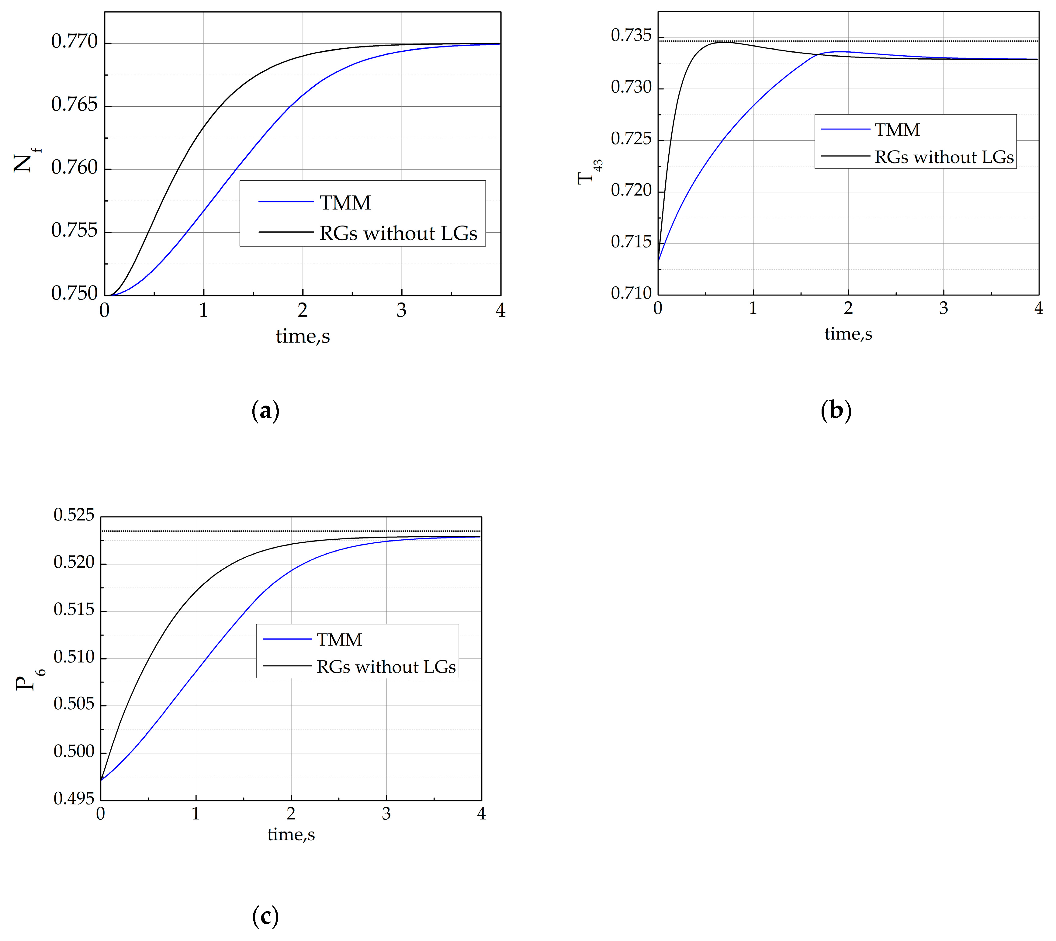
The tracking aim of all the simulations was to increase the fan speed by 2%. The simulations were set up in Matlab (R2012b) on a Windows 7 32 bit PC (CPU Core(TM) i3-4170 3.7 GHz, Memory 4 GB). Parameters of the feedback control for set-point tracking were given as $K_1=\left[\begin{array}{ccc}-3.4314& -11.2365& -0.3290\end{array}\right]$, $K_2=-0.3290$. We first illustrated the operation of the original RG and its advantages over the traditional Min–Max structure on a high fidelity turbofan engine model. The same main controller was implemented on the turbofan engine model and the original RG and Min–Max structure was designed for the same constraints limits, i.e., $T_{43\max }=0.7332$, $P_{6\max }=0.5210$. Figure 4 compares the performances of the original RG and the traditional Min–Max method. The response became less conservative and quicker when the original RG was used and all constraints were strictly enforced. More specifically, the limit would be as close as possible to the limit value using RG, while the traditional Min–Max method might cause the limit to be restricted prematurely before reaching the limit value.

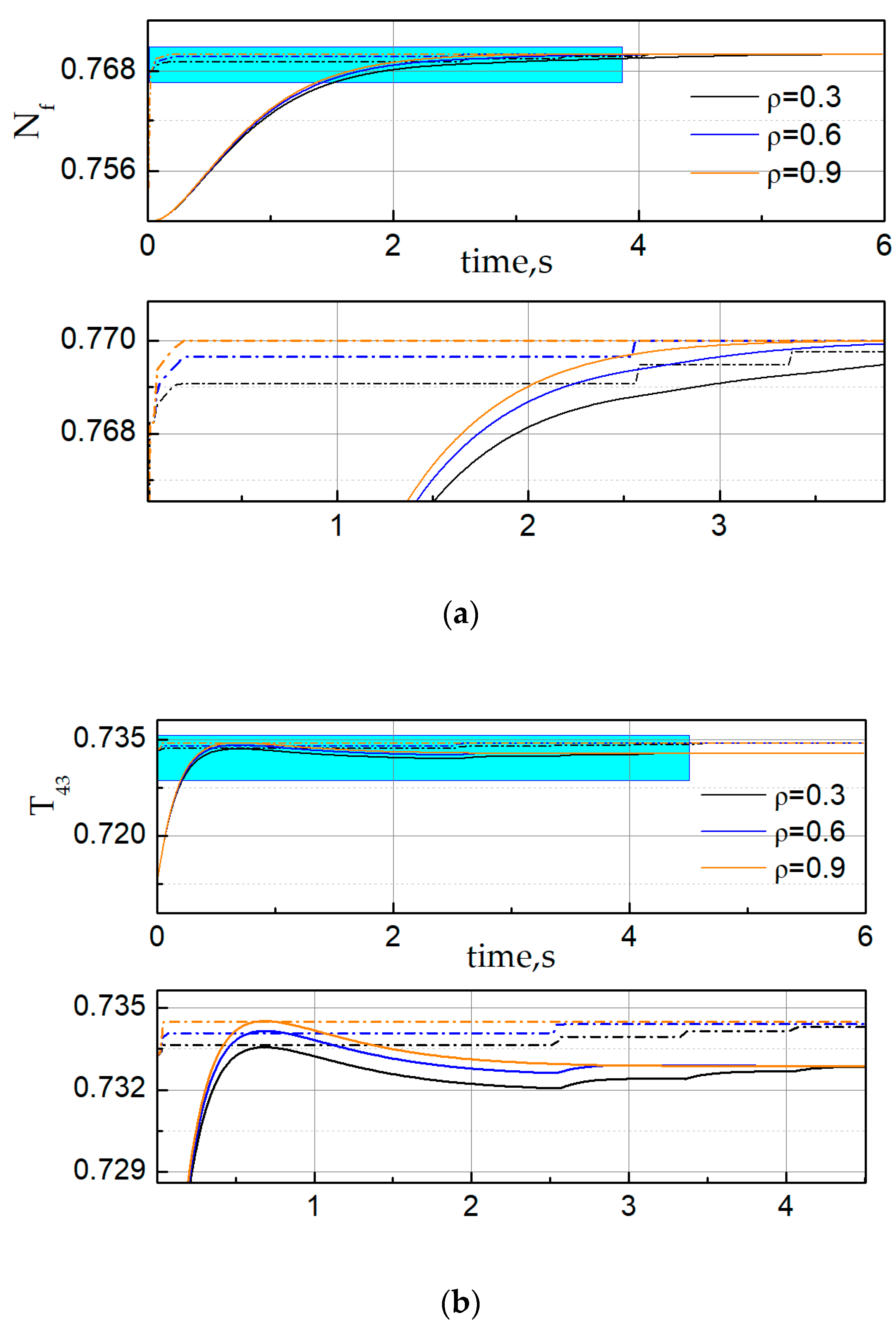
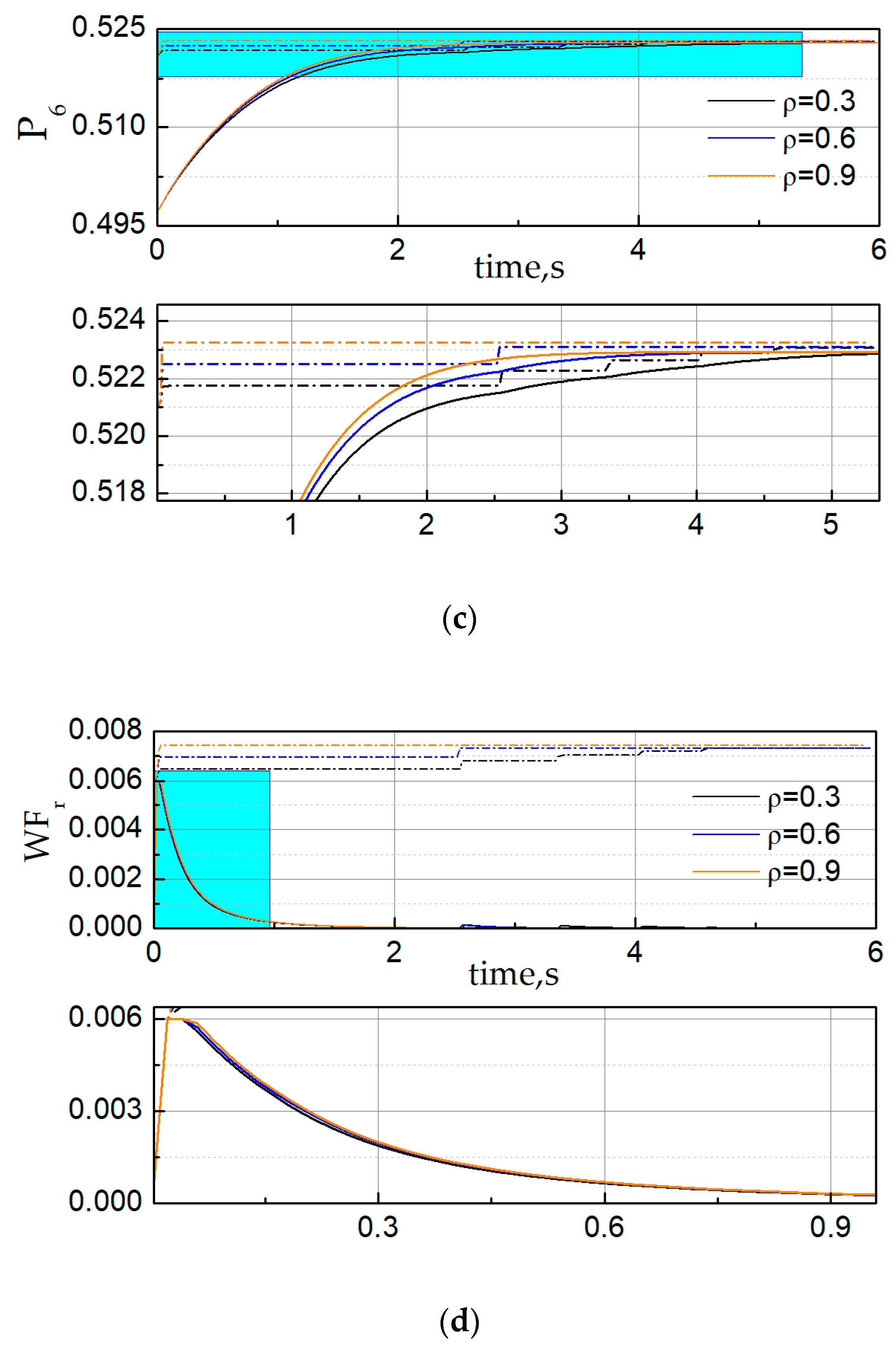
Secondly, we illustrated the influence of parameter design of LGs in handling varying constraints. Figure 5 compares the performances of RGs with LGs for different parameters $\rho$. To verify the validity of LGs, the temperature constraint, pressure constraint and rate of fuel flow constraint were designed as follows in the simulation:

$$\begin{gathered} T_{43\max }=0.7332, \\ {P}_{6\max }=0.5210, \\ W{F}_{r\max }=0.0060, \\ \alpha =0.0020,\beta =0.0048,\gamma =0.2667. \end{gathered}$$

From the simulation results we could observe that the fan speed could quickly track the reference speed within the parameter variation. The response became faster when the parameter $\rho$ was increasing and it showed that all constraints were almost enforced.

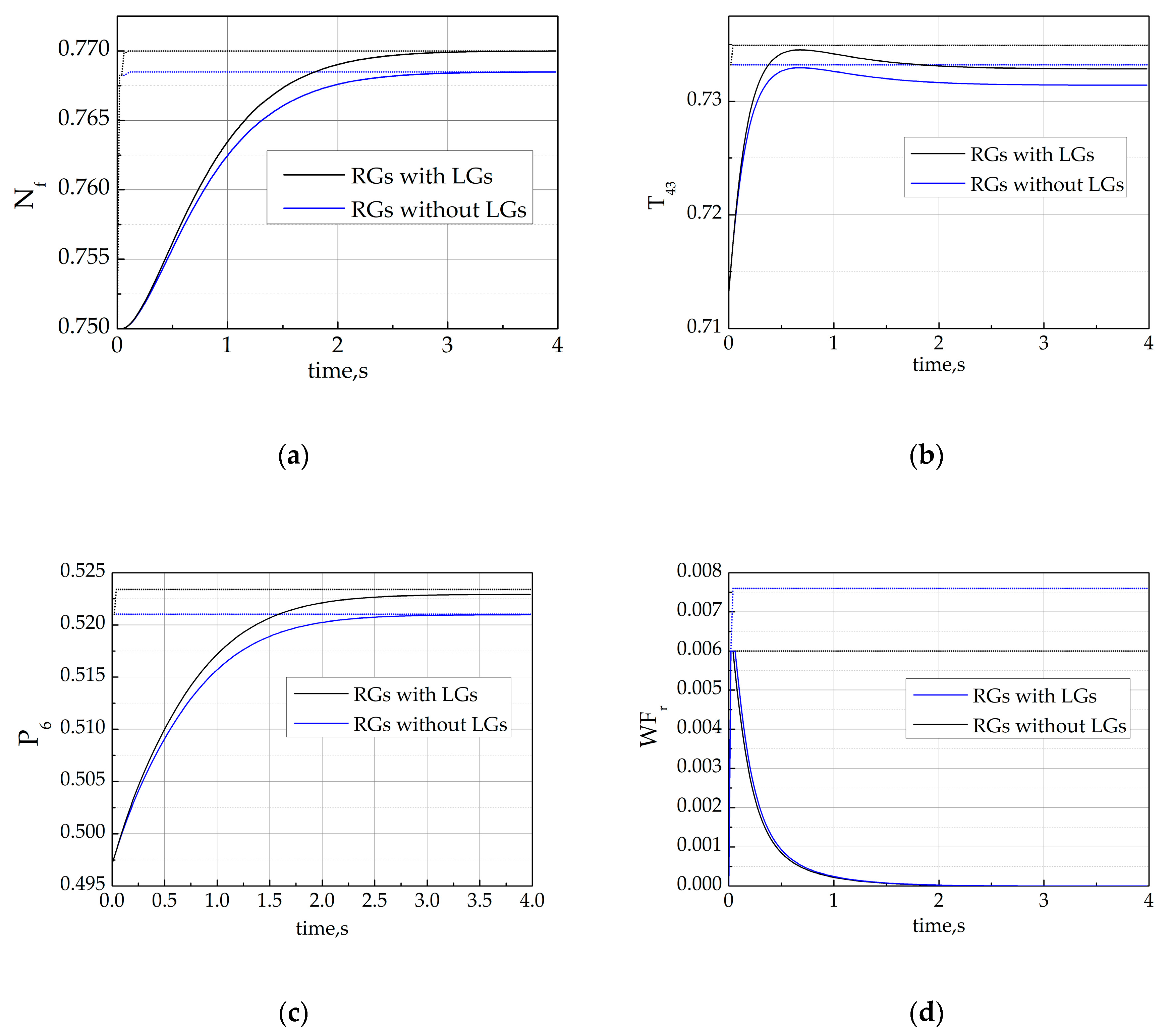
Finally, we illustrated the ancillary effects of LGs for RGs in enhancing the engine thrust. In this simulation, the temperature constraint, pressure constraint and rate of fuel flow constraint were designed as the same as the second simulation and steady violation condition would occur by the manual design of limits. Figure 6 compares the performances of RGs with and without LGs. As shown in Figure 6, $T_{43}$, $P_6$ and $W{F}_r$ rode the constraint boundary without LGs. However, due to steady violation, the fan speed failed to track the reference speed resulting in failing to obtain the required thrust. With LGs, the fan speed could quickly track the reference speed so that the engine thrust could be enhanced and all constraints were strictly enforced.

5. Conclusions

The paper illustrated the application and improvement of the recently developed reference governors for constraint handling in turbofan engines. To ensure the effective work of RGs, limit governors were proposed as add-on schemes that slack constraints when RGs were infeasible. The limit governor design method to guarantee the invariance of the output admissible set was studied in this paper. The reference governor with the limit governor rigorously enforced the constraints based on an accurate prediction model and the design method of output admissible sets. Simulation results, based on high fidelity engine models, confirmed the following points of this research: (1) The reference governor approach provided a faster and less conservatism response than the traditional min–max approach; (2) the proposed limit protection scheme could effectively track the reference, enhance the engine thrust when steady violation occurred and handled the constraints during transients and steady states.

References

- Richter, H. Advanced Control of Turbofan Engines; Springer: New York, NY, USA, 2012; pp. 137–147. [Google Scholar]
- Jaw, L.; Mattingly, J. Aircraft Engine Controls: Design, System Analysis, and Health Monitoring; American Institute of Aeronautics & Astronautics (AIAA): Reston, VA, USA, 2009; pp. 136–138. [Google Scholar]
- May, R.D.; Garg, S. Reducing conservatism in aircraft engine response using conditionally active min-max limit regulators. In Proceedings of the ASME Turbo Expo: Turbine Technical Conference and Exposition, Copenhagen, Denmark, 11–15 June 2012. [Google Scholar]
- Du, X.; Richter, H.; Guo, Y. Multivariable sliding-mode strategy with output constraints for aeroengine propulsion control. J. Guid. Control. Dyn. 2016, 39, 1631–1642. [Google Scholar] [CrossRef]
- Richter, H. Multiple sliding modes with override logic: Limit management in aircraft engine controls. J. Guid. Control. Dyn. 2012, 35, 1132–1142. [Google Scholar] [CrossRef]
- Qin, J.; Huang, J.; Pan, M. An optimal augmented monotonic tracking controller for aircraft engines with output constraints. Energies 2017, 10, 73. [Google Scholar] [CrossRef]
- Du, X.; Sun, X.-M.; Wang, Z.-M.; Dai, A.-N. A scheduling scheme of linear model predictive controllers for turbofan engines. IEEE Access 2017, 5, 24533–24541. [Google Scholar] [CrossRef]
- Richter, H.; Singaraju, A.V.; Litt, J.S. Multiplexed predictive control of a large commercial turbofan engine. J. Guid. Control. Dyn. 2008, 31, 273–281. [Google Scholar] [CrossRef]
- Kolmanovsky, I.; Merill, W. Limit protection in gas turbine engines based on reference and extended command governors. In Proceedings of the 50th AIAA/ASME/SAE/ASEE Joint Propulsion Conference, Cleveland, OH, USA, 28–30 July 2014. [Google Scholar]
- Kolmanovsky, I.; Weiss, A.; Merrill, W. Incorporating risk into control design for emergency operation of turbo-fan engines. In Proceedings of the Infotech@Aerospace 2011, St. Louis, MO, USA, 29–31 March 2011. [Google Scholar]
- Kolmanovsky, I.V.; Jaw, L.C.; Merrill, W.; Van, H.T. Robust control and limit protection in aircraft gas turbine engines. In Proceedings of the IEEE International Conference on Control Applications, Dubrovnik, Croatia, 3–5 October 2012. [Google Scholar]
- Tee, K.P.; Ge, S.S.; Tay, E.H. Barrier lyapunov functions for the control of output-constrained nonlinear systems. Automatica 2009, 45, 918–927. [Google Scholar] [CrossRef]
- Tian, Y.; Kolmanovsky, I. Reduced order and prioritized reference governors for limit protection in aircraft gas turbine engines. In Proceedings of the AIAA Guidance, Navigation, and Control Conference, National Harbor, MD, USA, 13–17 January 2014. [Google Scholar]
- Gong, X.; Kolmanovsky, I.; Garone, E.; Zaseck, K.; Chen, H. Constrained control of free piston engine generator based on implicit reference governor. Sci. China Inf. Sci. 2018, 61. [Google Scholar] [CrossRef]
- Hui, Y.; Mou, C.; Wu, Q.X. Flight envelope protection control based on reference governor method in high angle of attack maneuver. Math. Probl. Eng. 2015, 2015, 1–15. [Google Scholar] [CrossRef]
- Kalabic, U.V.; Buckland, J.H.; Cooper, S.L.; Wait, S.K.; Kolmanovsky, I.V. Reference governors for enforcing compressor surge constraints. IEEE Trans. Control Syst. Technol. 2016, 24, 1729–1739. [Google Scholar] [CrossRef]
- Garone, E.; Di Cairano, S.; Kolmanovsky, I. Reference and command governors for systems with constraints: A survey on theory and applications. Automatica 2017, 75, 306–328. [Google Scholar] [CrossRef] [Green Version]
- Kalabić, U.; Chitalia, Y.; Buckland, J.; Kolmanovsky, I. Prioritization schemes for reference and command governors. In Proceedings of the European Control Conference (ECC), Zürich, Switzerland, 17–19 July 2013. [Google Scholar]
- Gilbert, E.G.; Ong, C.-J. Constrained linear systems with hard constraints and disturbances: An extended command governor with large domain of attraction. Automatica 2011, 47, 334–340. [Google Scholar] [CrossRef]
- Guo, T.-H.; Litt, J.S. Risk management for intelligent fast engine response control. In Proceedings of the AIAA Infotech@Aerospace Conference, Seattle, WA, USA, 6–9 April 2009. [Google Scholar]
- Lu, F.; Zheng, W.; Huang, J.; Feng, M. Life cycle performance estimation and in-flight health monitoring for gas turbine engine. J. Dyn. Syst. Meas. Control 2016, 138. [Google Scholar] [CrossRef]
- Zhou, W.X. Research on Object-Oriented Modeling and Simulation for Aeroengine and Control System. Ph.D. Dissertation, Nanjing University of Aeronautics and Astronautics, Nanjing, China, 2007. [Google Scholar]
- Pang, S.; Li, Q.; Zhang, H.B. An exact derivative based aero-engine modelling method. IEEE Access 2018, 6, 34516–34526. [Google Scholar] [CrossRef]
- Pan, M.; Cao, L.; Zhou, W.; Huang, J.; Chen, Y.-H. Robust decentralized control design for aircraft engines: A fractional type. Chin. J. Aeronaut. 2019, 32, 347–360. [Google Scholar] [CrossRef]
- Tang, L.; Huang, J.; Pan, M. Switching LPV control with double-layer LPV model for aero-engines. Int. J. Turbo Jet-Engines 2016, 34, 313–320. [Google Scholar] [CrossRef]
- Lu, F.; Qian, J.; Huang, J.; Qiu, X. In-flight adaptive modeling using polynomial lpv approach for turbofan engine dynamic behavior. Aerosp. Sci. Technol. 2017, 64, 223–236. [Google Scholar] [CrossRef]
- Lin, Y.H.; Zhang, H.B. Establishment of state variable model of aeroengine with improved least square fitting. Appl. Mech. Mater. 2010, 40–41, 27–33. [Google Scholar] [CrossRef]
- Kalabic, U. Reference Governors: Theoretical Extensions and Practical Applications; Ford Motor Company: Dearborn, MI, USA, 2015. [Google Scholar]
- Gilbert, E.G.; Tan, K.T. Linear systems with state and control constraints: The theory and application of maximal output admissible sets. IEEE Trans. Autom. Control 1991, 36, 1008–1020. [Google Scholar] [CrossRef]
Figure 1.
Structure of the traditional Min–Max architectures.
Figure 2.
Structure of the novel architectures discussed in this paper.
Figure 3.
Comparisons of simulations with parameter perturbing under 2% step reference. (a) The time history of the rate of fan speed; (b) the time history of the rate of the high-pressure rotor speed; (c) the time history of fan speed; (d) the time history of high-pressure rotor speed; (e) the time history of the rate of fuel flow; (f) the time history of the rate of the high-pressure turbine outlet temperature and (g) the time history of the low-pressure compressor outlet pressure.
Figure 4.
Comparison of original references governors (RGs) and traditional Min–Max structure. (a) The time history of fan speed (solid line); (b) the time history of the high-pressure turbine outlet temperature (solid line) and corresponding limit (dot) and (c) the time history of the low-pressure compressor outlet pressure (solid line) and corresponding limit (dot).
Figure 5.
Comparison of RGs with limit governors (LGs) using different parameter values. (a) The time history of fan speed (solid line) and admissible reference command (dash dot); (b) the time history of the high-pressure turbine outlet temperature (solid line) and corresponding limit (dash dot); (c) the time history of the low-pressure compressor outlet pressure (solid line) and corresponding limit (dash dot) and (d) the time history of the rate of fuel flow (solid line) and corresponding limit (dash dot).
Figure 6.
Comparison between RGs with LGs and RGs without LGs. (a) The time history of fan speed (solid line) and admissible reference command (dot); (b) the time history of the high-pressure turbine outlet temperature (solid line) and corresponding limit (dot); (c) the time history of the low-pressure compressor (solid line) outlet pressure and corresponding limit (dot) and (d) the time history of the rate of fuel flow (solid line) and corresponding limit (dot).
© 2019 by the authors. Licensee MDPI, Basel, Switzerland. This article is an open access article distributed under the terms and conditions of the Creative Commons Attribution (CC BY) license (http://creativecommons.org/licenses/by/4.0/).
Share and Cite
MDPI and ACS Style
Xu, W.; Pan, M.; Qin, J.; Huang, J. Reference and Limit Governors for Limit Protection of Turbofan Engines. Energies 2019, 12, 2803. https://doi.org/10.3390/en12142803
AMA Style
Xu W, Pan M, Qin J, Huang J. Reference and Limit Governors for Limit Protection of Turbofan Engines. Energies. 2019; 12(14):2803. https://doi.org/10.3390/en12142803
Chicago/Turabian StyleXu, Wenhao, Muxuan Pan, Jiakun Qin, and Jinquan Huang. 2019. "Reference and Limit Governors for Limit Protection of Turbofan Engines" Energies 12, no. 14: 2803. https://doi.org/10.3390/en12142803
Note that from the first issue of 2016, this journal uses article numbers instead of page numbers. See further details here.