Article

Better Fuel Economy by Optimizing Airflow of the Fuel Cell Hybrid Power Systems Using Fuel Flow-Based Load-Following Control

1
Faculty of Electronics, Communication and Computers, University of Pitesti, 1 Targu din Vale, 110040 Pitesti, Romania
2
University Politehnica of Bucharest, 313 Splaiul Independentei, 060042 Bucharest, Romania
3
Renewable Energy Research Centre (RERC), King Mongkut’s University of Technology North Bangkok, Bangkok 10800, Thailand
4
Gazi University, Faculty of Technology, Department of Electrical and Electronics Engineering, 06500 Teknikokullar, Ankara, Turkey
*
Author to whom correspondence should be addressed.
Energies 2019, 12(14), 2792; https://doi.org/10.3390/en12142792
Submission received: 23 June 2019 / Revised: 13 July 2019 / Accepted: 16 July 2019 / Published: 19 July 2019
(This article belongs to the Special Issue Fuel Cell Renewable Hybrid Power Systems)

Abstract

:
In this paper, the results of the sensitivity analysis applied to a fuel cell hybrid power system using a fuel economy strategy is analyzed in order to select the best values of the parameters involved in fuel consumption optimization. The fuel economy strategy uses the fuel and air flow rates to efficiently operate the proton-exchange membrane (PEM) fuel cell (FC) system based on the load-following control and the global extremum seeking (GES) algorithm. The load-following control will ensure the charge-sustained mode for the batteries’ stack, improving its lifetime. The optimization function’s optimum, which is defined to improve the fuel economy, will be tracked in real-time by two GES algorithms that will generate the references for the controller of the boost DC-DC converter and air regulator. The optimization function and performance indicators (such as FC net power, FC electrical efficiency, fuel efficiency, and fuel economy) have a multimodal behavior in dithers’ frequency. Furthermore, the optimum in the considered range of frequencies depends on the load level. So, the best value could be selected as the frequency where the optimum is obtained for the most load levels. Considering a dither frequency of 100 Hz selected as the best value, the sensitivity analysis of the fuel economy is further analyzed for different values of the weighting parameter keff, highlighting the multimodal feature in the parameters for the optimization function and fuel economy as well. A keff value around of 20 lpm/W seems to give the best fuel economy in the full range of load.

Graphical Abstract

1. Introduction

Instead of a diesel generator [1], the proton-exchange membrane fuel cell (PEM FC) system could be used as a backup green energy source [2] for an FC hybrid power system (FC HPS) to mitigate the load variability by the load-following (LF) control [3,4,5]. A hybrid energy storage system (ESS) using batteries and ultracapacitors is mandatory to dynamically compensate the power flow balance [6,7]. The most used ESS topologies are the active and semi-active topologies, using two and one bidirectional DC-DC converters integrated into a multiport topology, respectively [8,9,10]. An active topology with two bidirectional DC-DC converters is more flexible as a control structure compared to a semi-active topology [9]. The two control references will be generated by the energy management strategies (EMS), usually to regulate the DC voltage and mitigate the load pulses via the bidirectional DC-DC converters for the batteries and ultracapacitors stacks [5,7,11,12]. The EMS has an important role in the optimal and safe operation of the FC system [13,14]. The control objectives for PEM FC system are as follows [15,16,17]: (1) minimization of the fuel consumption; (2) supplying the dynamic loads with energy, such as FC vehicles; (3) safe operation by using appropriate control loops to mitigate the load pulses, to limit the FC current slope, and to avoid fuel starvation.
The first objective can be ensured using a real-time optimization (RTO) strategy based on different optimization functions, which integrate performance indicators related to fuel consumption such as FC net power, FC lifetime, and cost [18,19,20].
The equivalent consumption minimization strategy (ECMS) is a well-known strategy applied to FC vehicles, which converts the energy difference in battery charging (at the start and end of a load cycle) into additional fuel consumption, to compensate this loss of energy by discharging the battery [21]. In last decade, several algorithms searching for the global optimum using different optimization functions have been proposed in the literature [22,23,24]. Intelligent concepts are usually involved in these algorithms [25,26,27]. In this study, the global extremum seeking (GES) algorithm is used due to the good performance reported in the previous work for FC systems [28,29,30,31], photovoltaic (PV) systems [22,23,32], and wind turbine (WT) systems [33,34].
The objective of this paper is to use the sensitivity approach to identify the best value of the parameters used by the optimization function and control loops. Except the tuning parameters of the GES algorithm, which will be designed to ensure the imposed performance and stability of the tracking loops, the dither’s frequency fd is the most important parameter that could dynamically affect the performance of the GES algorithm.
The GES algorithm must search the optimization function’s optimum in real-time, which is defined in this study as a weighted function of the FC net power and the fuel consumption efficiency using the weighting parameters knet and keff. So, if knet = 1, then it is important to know the value of the weighting parameter keff, where the best fuel economy is obtained. So, the sensitivity approach in this study will be performed using the parameters fd and keff.
The structure of the paper is as follows. The FC HPS architecture and LF control and optimization loops are briefly presented in Section 2. The EMS based on LF control and optimization loops is detailed in Section 3. The obtained results are presented and discussed in Section 4. Section 5 concludes this study.

2. FC Hybrid Power System

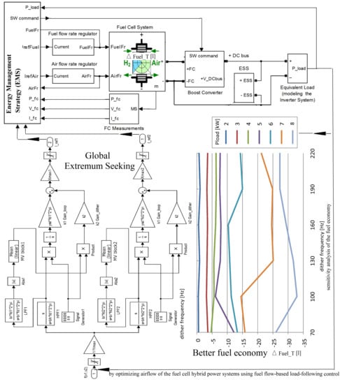
The synoptic architectures of the FC HPS and ESS are presented in Figure 1a. The FC power delivered on the DC can be controlled via the boost converter using the switching (SW) command generated by the boost controller under the EMS proposed in this paper. Also, the generated FC power depends on the fuel and air regulators controlled by the input references IrefFuel and IrefAir.
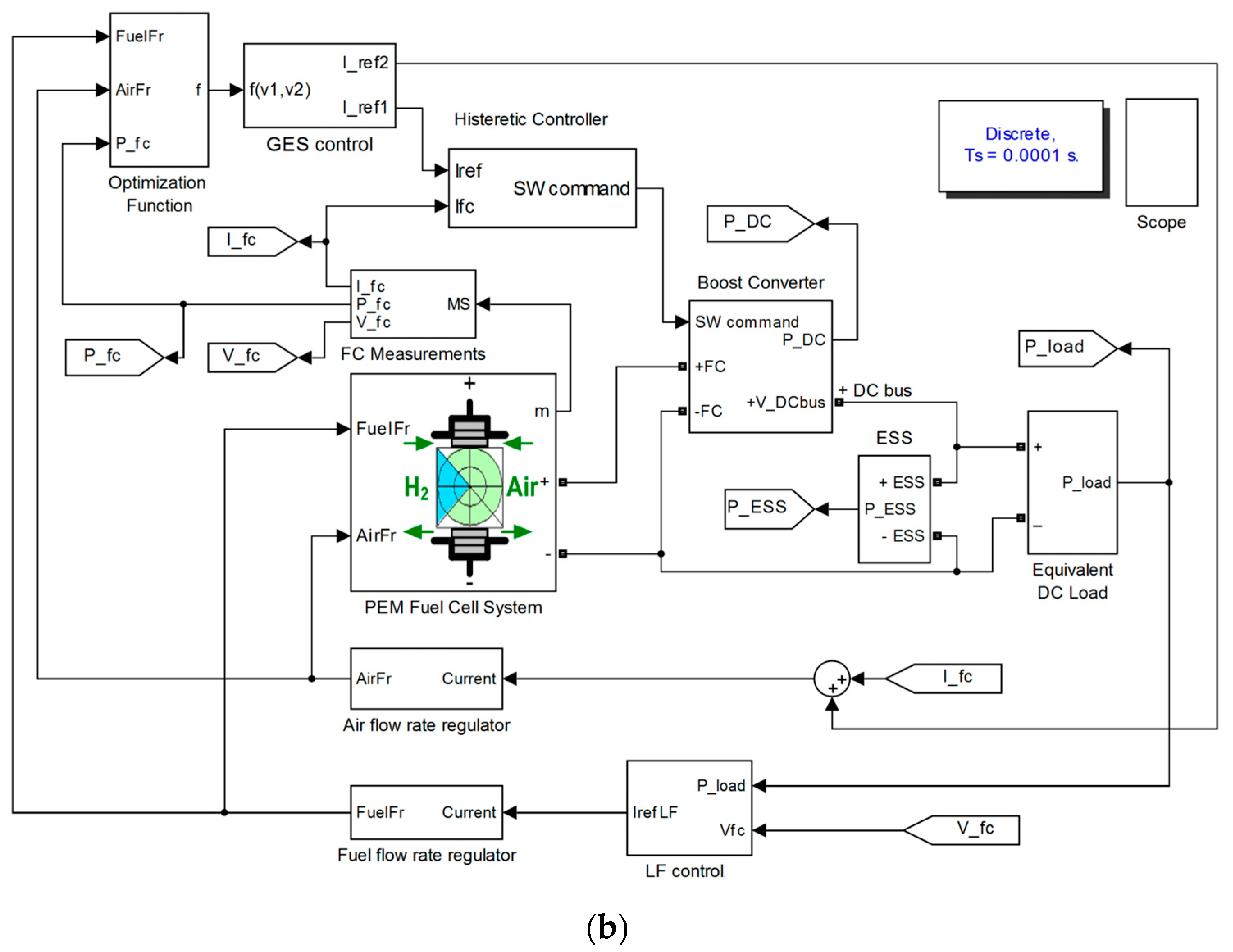
The Matlab-Simulink® diagram of the FC HPS architecture is presented in Figure 1b. The FC system is the main energy source to supply the load demand on the DC bus, which is modeled by an equivalent DC load for the inverter and an AC load in order to speed up the simulation.
The LF control will set the current reference IrefLF for the fuel flow rate (FuelFr) regulator to comply with the power flow balance on the DC bus (1), with the battery operating in charge-sustaining mode (2):
C D C u d c d u d c / d t   =   η b o o s t p F C g e n +   p E S S   p l o a d ;
P E S S ( A V ) 0 .
So, considering (2), (1) will be rewritten in the average value (AV) during a load cycle (LC) as (3):
0 =   η b o o s t P F C g e n ( A V )   P l o a d ( A V ) P F C g e n ( A V ) = P l o a d ( A V ) / η b o o s t .
Thus, the FC current generated by the FC system will be given by (4):
I F C ( A V ) = P l o a d ( A V ) /   ( η b o o s t V F C ( A V ) ) .
Consequently, the current reference IrefLF will be estimated by the LF control using the AV filtering method, based on the mean value (MV) technique of the FC current during a dithers’ period:
I r e f L F I F C ( A V ) =   P l o a d ( A V ) / ( η b o o s t V F C ( A V ) )
The MV technique or another filtering technique can be used to smooth the values used in (5) for the safe operation of the FC system, thus avoiding fuel starvation due to sharp changes in load demand. The current reference IrefLF will set the fuel flow rate FuelFr value using the FuelFr regulator’s relationship (6):
F u e l F r = 60000 R ( 273 + θ ) N C I L F r e f 2 F ( 101325 P f ( H 2 ) ) ( U f ( H 2 ) / 100 ) ( x H 2 / 100 ) .
Because of (5),
I F C I F C ( A V ) I r e f L F .
So, the current reference Iref2 will optimally adjust the air flow rate (AirFr) value using the AirFr regulator’s relationship (8):
A i r F r = 60000 R ( 273 + θ ) N C ( I F C + I r e f 2 ) 4 F ( 101325 P f ( O 2 ) ) ( U f ( O 2 ) / 100 ) ( y O 2 / 100 ) .
Thus, the input references of the fueling regulators are set as follows: IrefFuel = IrefLF and IrefAir = IFC + Iref2.
The optimization function’s optimum (computed in the block called “optimization function”, in Figure 1) will be searched using the current reference Iref1 that will set the FC current based on the 0.1 A hysteresis controller for the boost DC-DC converter.
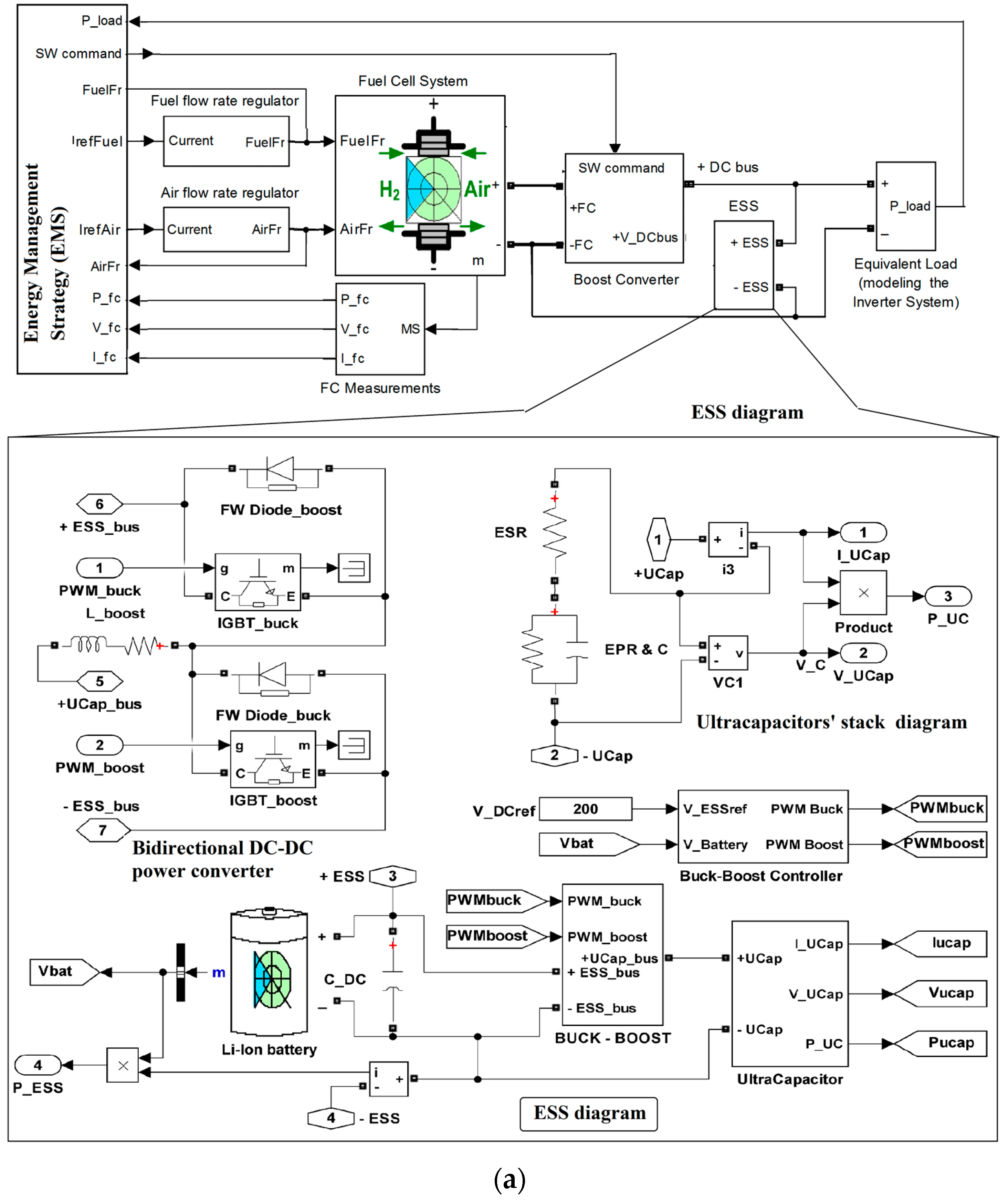
A semi-active 100 Ah battery/100 F ultracapacitors ESS topology was chosen to dynamically compensate power in (1) and stabilize the DC voltage at 200 V (uDC ≅ 200 V). The battery will operate in charge-sustaining mode due to the LF control applied to the fuel regulator (6), which will set the FC power close to the requested FC power on the DC bus. The FC power is P F C g e n ( A V ) given by (3) if (2) is considered. Thus, the battery will compensate the minor imbalance in energy flow on the DC bus (1) due to the changes in load profile or the small difference between the FC current set by the LF control (5) I F C I L F r e f I F C ( A V ) =   P l o a d ( A V ) / ( η b o o s t V F C ( A V ) ) and the value I F C + I r e f 2 set by the GES-based optimization loop (which is applied to the air regulator (7)). So, a 100 Ah capacity of the battery has been obtained for a 1 kW imbalance in energy flow during a 12 s load cycle using the design relationships from [5,7]. This capacity is more than sufficient, considering the sizing design presented in [2]. The sharp changes in load profile, such as pulses, can produce an imbalance in power flow on the DC bus (1) due to the large response time of the FC system and the battery, which is in the order of hundreds of milliseconds and tens of minutes, respectively. During the transitory regimes of the FC system and battery, the ultracapacitors’ stack will dynamically compensate the power flow on the DC bus (1) via the bidirectional DC-DC power converter. The 100 F capacitance was obtained for a 1 kW/100 ms pulse using the design relationships from [5,7]. The DC voltage regulation was implemented on the ultracapacitors’ stack side due to the slow response of the FC system, but also because the controlled inputs AirFr and FuelFr (via the fueling regulator) of the FC system and the controller of the FC boost converter are involved in the LF and optimization loops. Thus, if the DC voltage regulation will be implemented on the FC system’s side using a proportional–integral–derivative (PID) compensation technique of one of the aforementioned loops, then a degradation of the performance indicators will be obtained compared with the cases when the DC voltage regulation is implemented on the ultracapacitors’ stack side or on the battery’s side if an active ESS topology is selected instead of a semi-active type. If an active mitigation of the pulses on the DC bus must be implemented, then an active control of the bidirectional DC-DC power converter should be implemented in order to generate an anti-pulse from the ultracapacitors’ stack [5,7]. In this case, the DC voltage regulation remains to be implemented on the battery side using a PID compensation technique of the control designed to compensate the minor imbalance in energy flow on the DC bus (1). The high frequency ripple on the DC voltage will be mitigated in all cases by a 100 μF capacitor (CDC) designed using the design relationships from [5,7].
The FC parameters ( N C , θ , U f ( H 2 ) , U f ( O 2 ) ,   P f ( H 2 ) , P f ( O 2 ) , x H 2 , y O 2 ) were set for a 6 kW FC system, and R = 8.3145 J/(mol K) and F = 96485 As/mol are two well-known constants. The energy efficiency of the boost DC-DC converter may be considered constant in this study (ηboost = 0.9), because the boost controller operated in continuous current mode in the load range higher than 1 kW (so the case of light load was not considered), where the energy efficiency may vary in the range of 88% to 92%, but without significantly modifying the results obtained for a constant efficiency (as will be explained in the Discussion section).
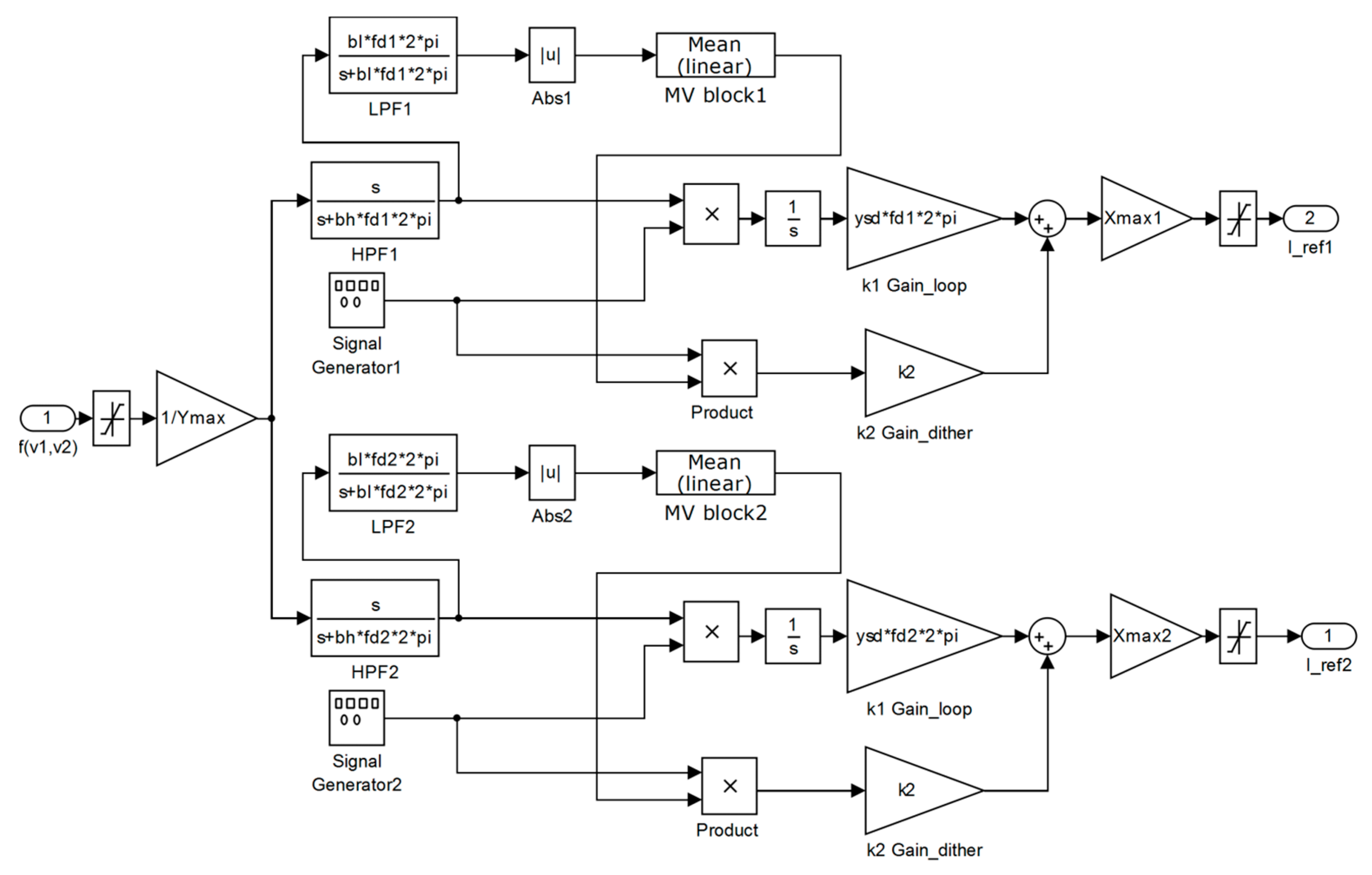
The current references Iref1 and Iref2 were generated by the GES controller shown in Figure 2, as will be explained in next section.

3. Energy Management Strategy

Each GES control was implemented (see Figure 2) based on the relationships from [30]. The dither’s frequencies were chosen to be fd1 = 100 Hz and fd2 = 2fd1 = 200 Hz in order to improve the dithers’ persistence by interference of the harmonics due to the nonlinear characteristics of the FC system. The cut off frequencies of the low-pass filter (LPF1 and LPF2 in Figure 2) and the high-pass filter (HPF1 and HPF2 in Figure 2) were set by the parameters bl = 1.5 and bh = 0.1. The tuning parameters were designed based on relationships presented in [30], as follows: k1 = 1, k2 = 2. The normalization values of the input (the optimization function y = f ( v 1 , v 2 ) , where v1 and v2 are the search variables) and the outputs (the reference currents I r e f 1 and I r e f 2 for the boost controller and the air regulator) were set to k N f = 1 / Y max   =   1 / 100 0 , k N v 1 = X max 1 =   50 and k N v 2 = X max 2 =   2 0 . The normalization values were not strict, because the GES control was of the adaptive type, but choosing the right value would improve the searching speed. Readers interested in analyzing and designing a GES control for FC systems or PV, WT, and PV/WT FC HPSs may read [14,17] or [22,23,32], [33], and [35], respectively.
The searching speed was limited to 100 A/s by the slope limiters included in the FuelFr and AirFr regulators in order to ensure the safe operation of the PEM FC system. So, the FC current could increase up to 20 A during the FC time constant (TFC) of 0.2 s. The GES algorithm needed about 10 periods of dither (Td) to find the Global Maximum Power Point (GMPP) of the PV system for different steps in irradiance (because there was no limitation related to searching slope in this case, excepting the safe values given by the devices used in the boost the boost DC-DC power converter, which were very high compared to 100 A/s) [22,23]. Considering 10 dither periods to find the maximum efficiency point (MEP) of the FC system or the optimization function’s optimum (which is defined in relation to the FC system’s performance indicators), to avoid limitation due to FC response time, it was recommended to choose:
T d ( max ) T F C / 10 .
This means Td(max) ≅ 20 ms, so fd(min) ≅ 50 Hz. The maximum frequency of the dither would be considered fd(max) = 200 Hz in order to have an acceptable increment per dithers’ period (about 0.5 A per Td(min) = 5 ms). So, the frequency range of the dither was 70 Hz to 220 Hz, with a 30 Hz step in evaluation of the fuel economy based on the optimization function f defined by (10) [35]:
f ( x , A i r F r , F u e l F r , P L o a d ) = k n e t P F C n e t + k f u e l F u e l e f f ;
x ˙ = g ( x , A i r F r , F u e l F r , P L o a d ) , x X ;
where (11) models the dynamic part of the FC HPS [36], x is the state vector, and PLoad is the disturbance. The weighting coefficients knet (1/W) and kfuel (liters per minute (lpm)/W) were defined in accordance with the chosen EMS objective. For example, the FC system energy efficiency ( η s y s =   P F C n e t /   P F C ) was maximized if knet = 1 and kfuel = 0 (in this case f = PFCnet). If knet = 1 and kfuel ≠ 0, then the fuel consumption efficiency (Fueleff ≅ PFCnet / FuelFr) was also considered in the optimization function. So, it was possible to improve the fuel economy for a value of the kfuel weighting coefficient in range 5 lpm/W to 50 lpm/W, with 5 lpm/W step in evaluation of the fuel economy.
The LF control was implemented based on (5) in order to set the value of the FC net power requested by power flow balance (3). So,
P F C g e n = P F C n e t P l o a d   / η b o o s t ,
where,
P F C n e t P F C   P c m ;
P c m = I c m V c m = ( a 2 A i r F r 2 + a 1 A i r F r + a 0 ) ( b 1 I F C + b 0 ) .
The air compressor power (Pcm) was estimated with (14), considering the coefficients [37]: a 0 = 0.6 , a 1 = 0.04 , a 2 = 0.00003231 , b 0 =   0.9987 , and b 1 =   46.02 .
In order to not exceed the maximum FC power, the range of the load demand was considered from 2 kW to 8 kW, with a 1 kW step in the evaluation of the fuel economy.
The total fuel consumption, F u e l T = F u e l F r ( t ) d t , will be estimated in the next section for different load levels in order to evaluate the fuel economy, measured in liters (L).

4. Results

The values of the performance indicators P F C n e t , η s y s , F u e l e f f , and F u e l T using different dither’s frequencies and constant load levels are recorded in Table 1, Table 2, Table 3 and Table 4. The values obtained by simulation using the static feed-forward (sFF) strategy [
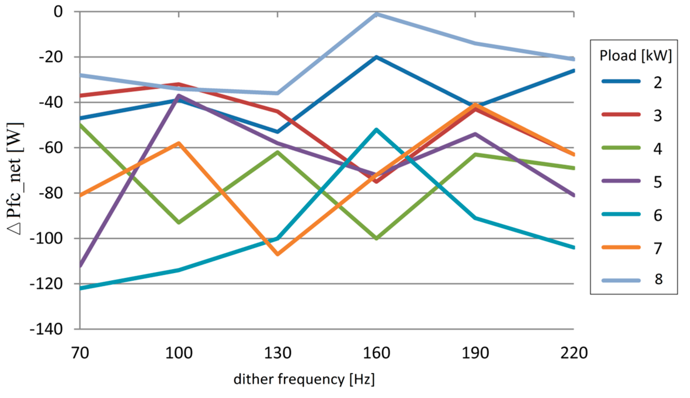
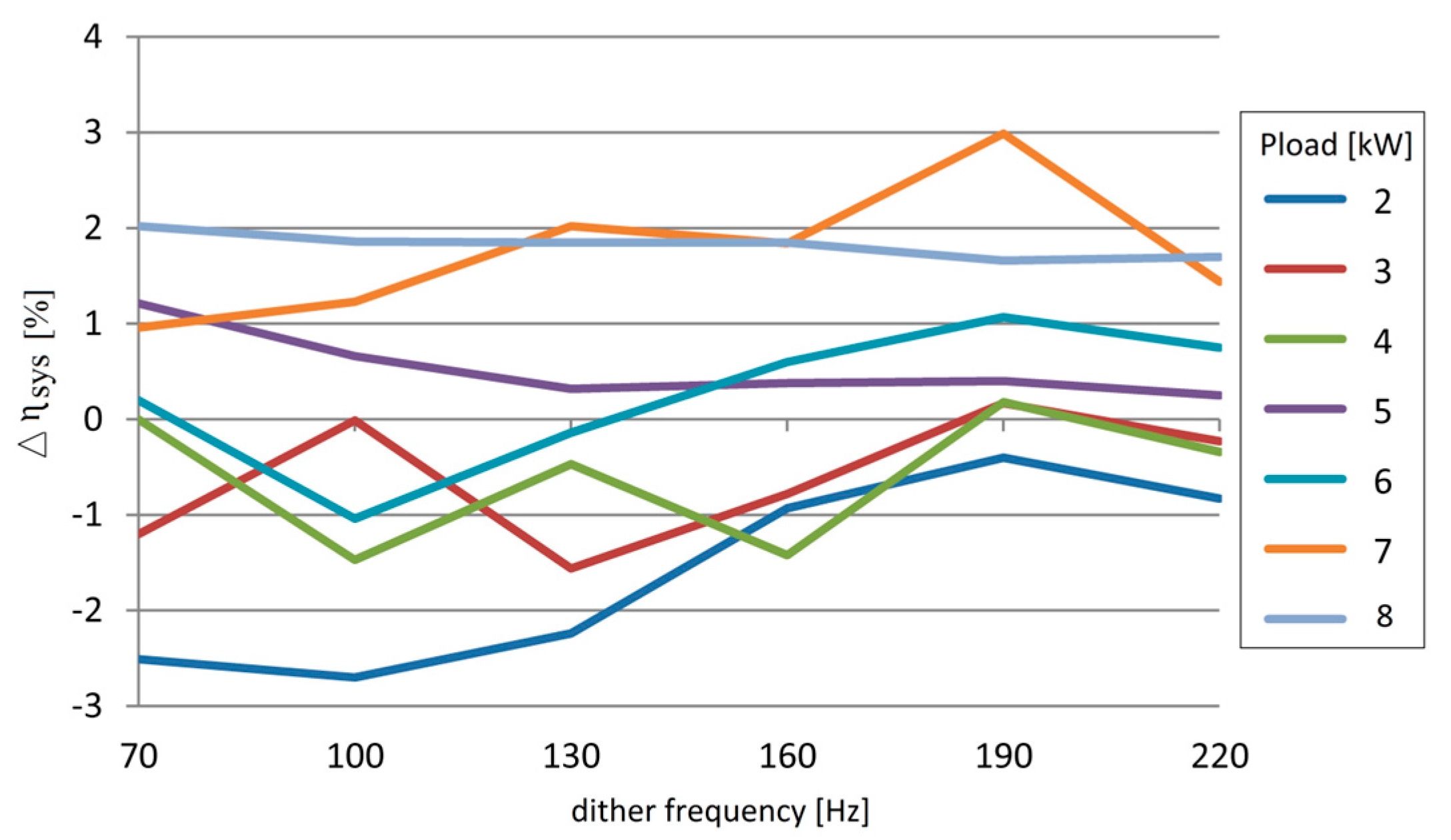
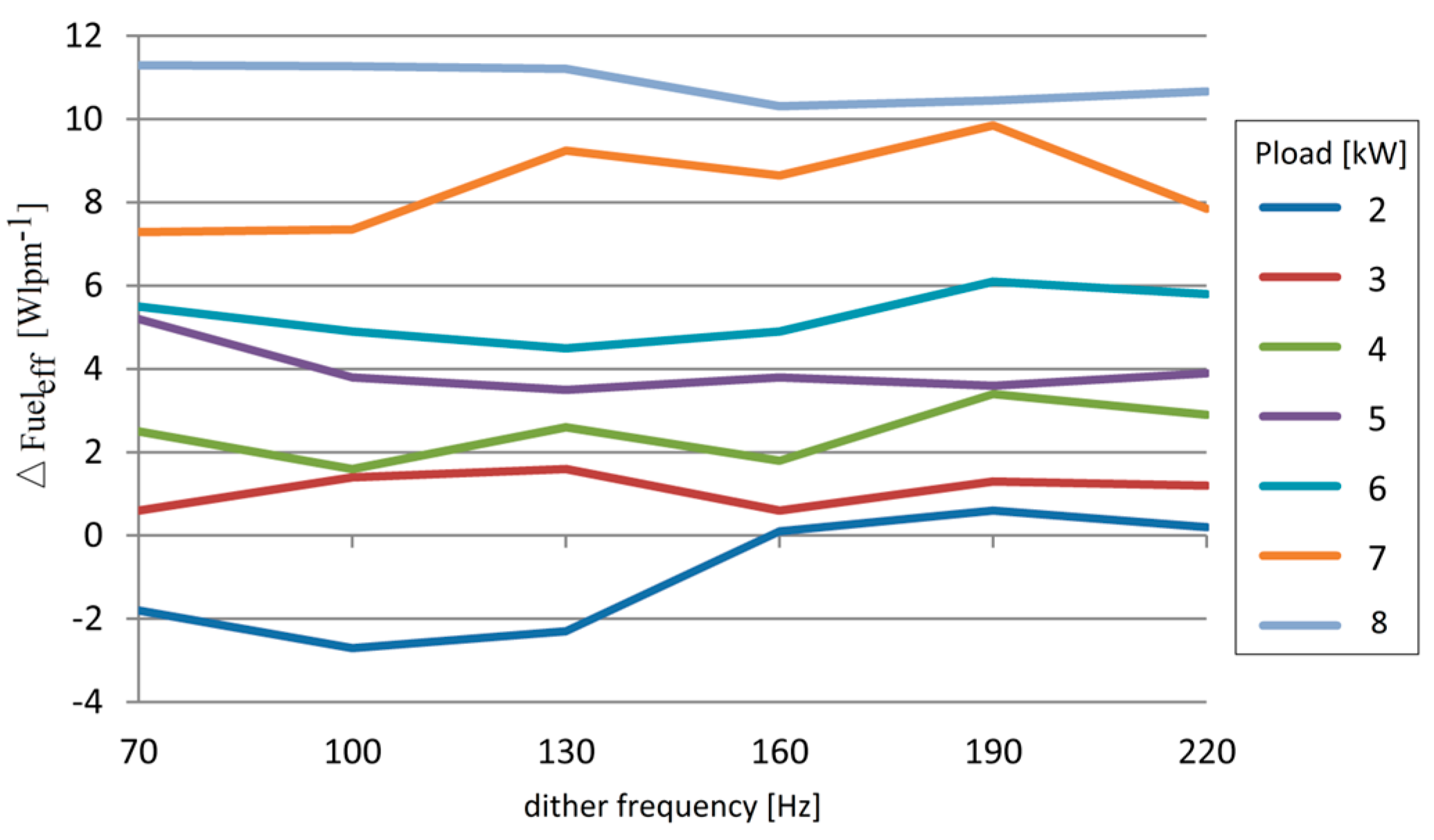
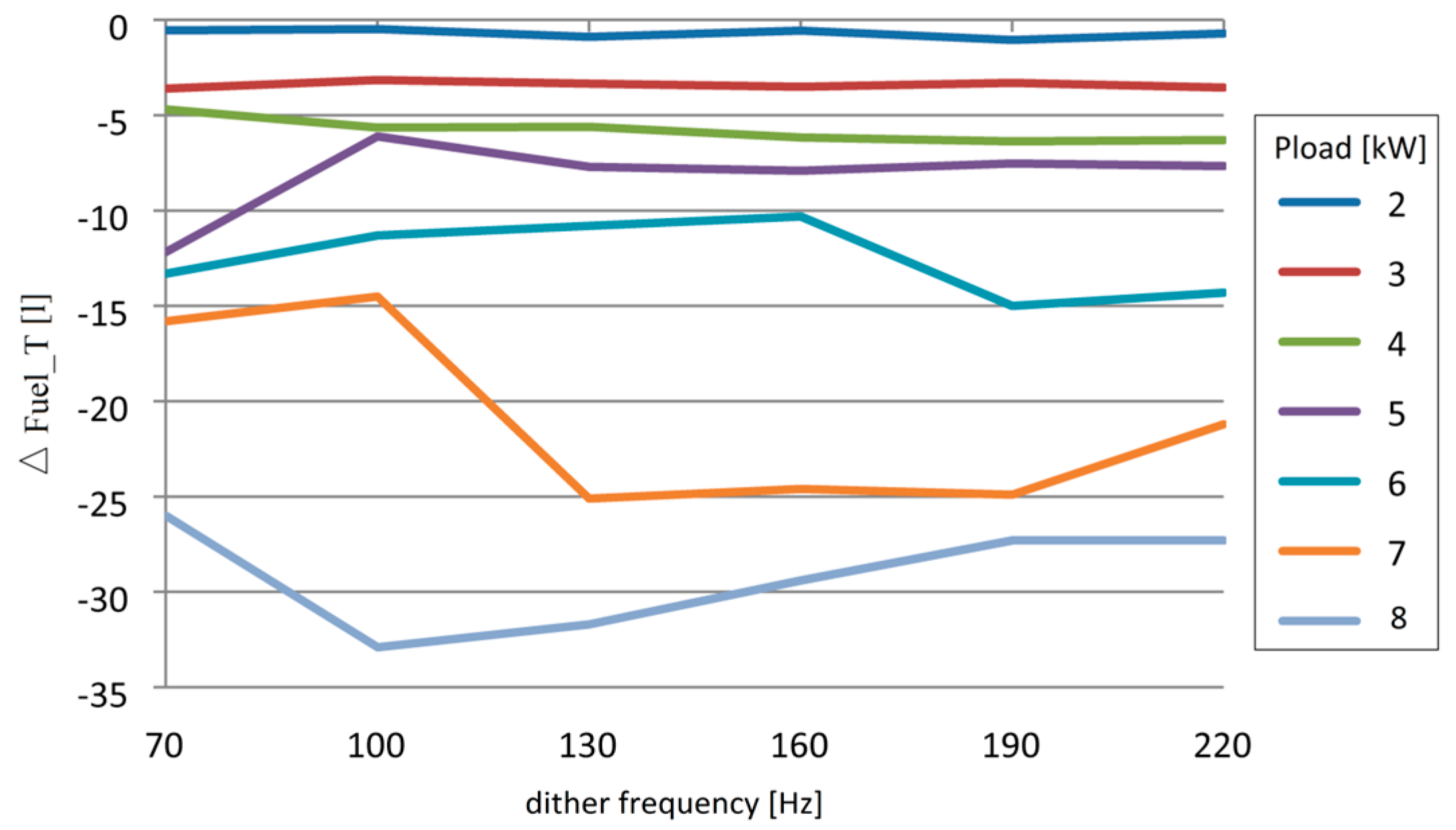
36], which is considered in this study as a reference strategy because it is the most known strategy implemented in commercial FC systems, are mentioned in the first column of these Tables. The differences in the performance indicators will be defined compared to the sFF strategy by using (15):
Δ P F C n e t P F C n e t   P F C n e t 0 ;
Δ η s y s = η s y s η s y s 0 ;
Δ F u e l e f f =   F u e l e f f   F u e l e f f 0 ;
Δ F u e l T =   F u e l T   F u e l T 0 .
The differences are recorded in Table 5, Table 6, Table 7 and Table 8 and represented in Figure 3, Figure 4, Figure 5 and Figure 6. Note the multimodal behavior in dithers’ frequency for all performance indicators. Also, it is worth mentioning that the optimum’s position (maximum of Δ P F C n e t , Δ η s y s , Δ F u e l e f f , and minimum of Δ F u e l T ) depends on the load level. So, the best value in the frequencies’ range could be selected as the frequency where the optimum is obtained for most of load levels, and this seems to be the dither frequency of 100 Hz.
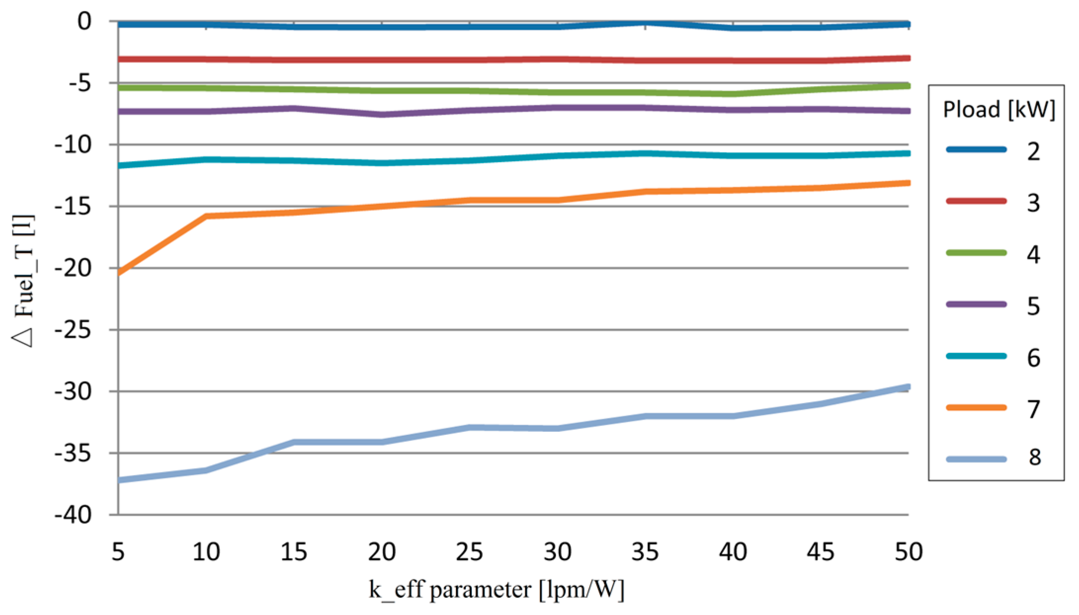
Considering a dither frequency of 100 Hz, the total fuel consumption ( F u e l T ) for different values of the parameters keff and Pload is recorded in Table 9. The values for keff = 0 (mentioned in the first column of the Table 9) are used as reference values. So, the differences in total fuel consumption ( Δ F u e l T ) are estimated in Table 10 and represented in Figure 7.
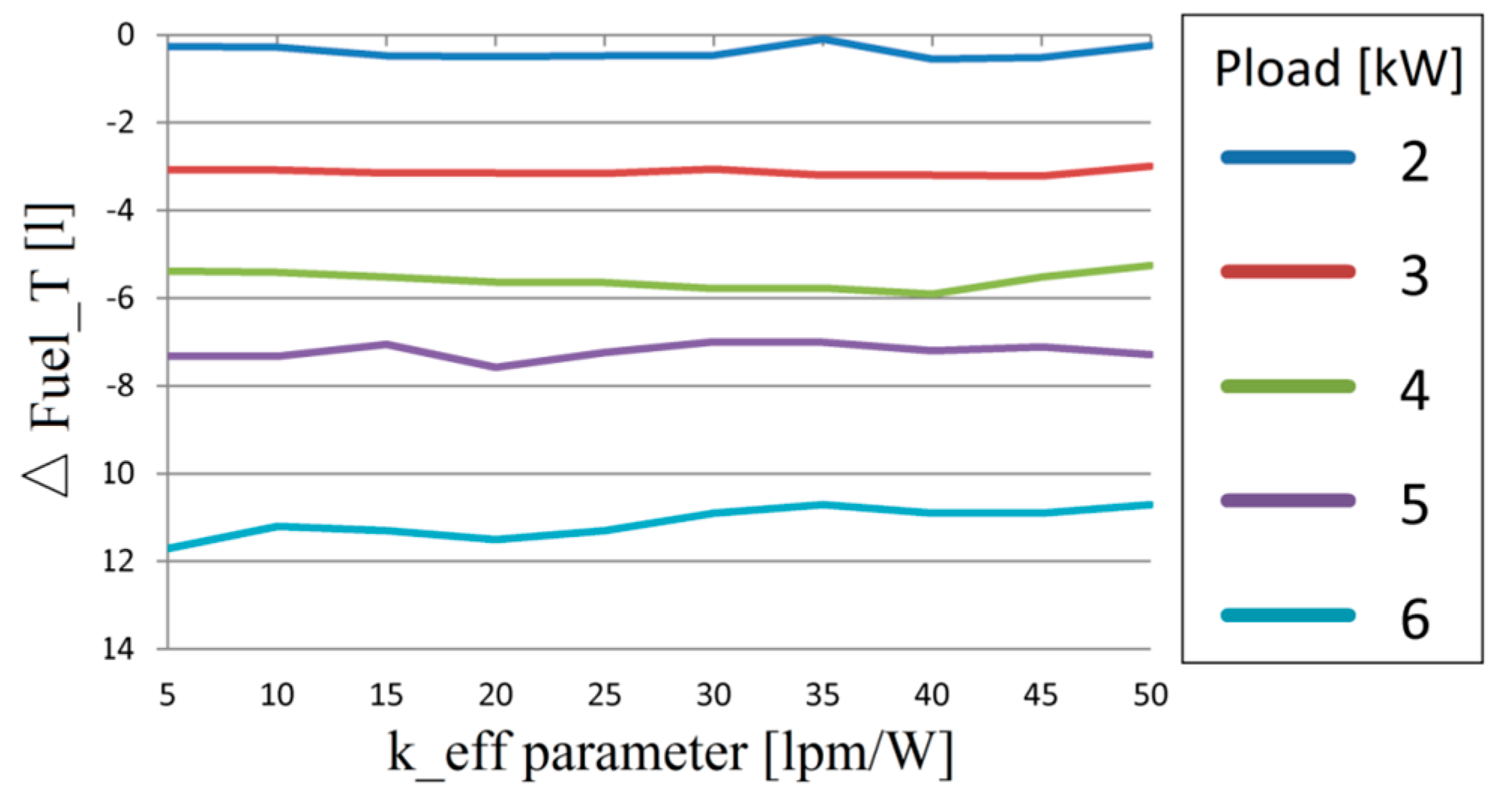
The sensitivity analysis of the fuel economy ( Δ F u e l T ) highlights the better fuel economy with increase in load level, and this is normal. Also, note the multimodal behavior in the weighting parameter keff. This is better shown in Figure 8 (where the high values of fuel economy for a load of 7 kW and 8 kW are canceled). Looking to Table 10 (where the optimum, local minimums, and the minimums at keff = 5 and keff = 50 are highlighted in different colors: yellow, blue, and gray, respectively), a keff value in the range of 20 lpm/W to 30 lpm/W seems to give the best fuel economy in the load range of 2 kW to 5 kW. However, note the decrease in fuel economy with the increase in keff value. So, the recommended value for the entire load range is keff = 20 lpm/W.
The effect of a variable energy efficiency of the boost converter on the results obtained at constant energy efficiency will be analyzed and discussed in the next section.

5. Discussion

The dependence of the power loss (Ploss) and energy efficiency for a DC-DC power converter were analyzed for low and medium power applications in [38,39] and [40,41,42], respectively. The main findings of the aforementioned studies are as follows:
1)
The energy efficiency characteristic related to the load current (Iload) is dependent on the control mode used, the switching frequency, and coil inductance [42];
2)
For low [38] and high [39] power applications using the control mode based on the pulse width modulation technique and optimal control, respectively, the energy efficiency can be approximated by (16):
η c o n v e r t e r = η max η max η min 4 lg 2 ( I l o a d I l o a d ( o p t ) ) ,
where ηmax is the maximum of the energy efficiency (obtained at the optimal load current Iload(opt)) and ηmin is the minimum of the energy efficiency (obtained in the considered load range).
3)
For low-power applications using the control mode based on the pulse frequency modulation technique, the energy efficiency can be approximated by (17) [38,39]:
η c o n v e r t e r = η max ζ η I l o a d ,
where ηmax is the maximum energy efficiency (obtained at the maximum load current Iload(max)) and ζη is a parameter (that must be determined using the experimental values in the considered range of load). Relationship (17) highlights the nonlinear increase in energy efficiency in the range of light loads and the saturation that appears in the rest of the load range;
4)
For most types of control used in medium and high-power applications, the energy efficiency in the normal load range (therefore, except for light loads), where the converter operates in continuous current mode [43,44], can be considered as constant or linearly increasing (18):
η c o n v e r t e r = η min + χ η I l o a d I l o a d ( max ) ,
where ηmin is the energy efficiency obtained at the load current Iload(min), which is the upper limit of light loads, and χη is a parameter to be determined using the experimental values in the considered load range (except the light loads).
The assumption that the energy efficiency linearly increases is valid for the medium-power FC HPS analyzed in this paper, because the load range was higher than 1 kW (so the case of light load was not considered). For different values of the load current, the LF control and optimization loops set the values of the FC current, IFC0, and IFC1, using the sFF strategy and the fuel economy strategy analyzed in this paper. So, (18) can be rewritten using as a variable the FC current as (19):
η b o o s t = η min + K η I F C I F C ( max ) ,
where ηmin ≅ 88.5% is the energy efficiency obtained at the nominal FC current, IFC(min) ≅ 30 A, and Kη = 4 is a parameter which has been determined using the experimental values of the energy efficiency ηmax ≅ 92% obtained at the maximum FC current, IFC(max) ≅ 240 A. Note that the energy efficiency obtained at the nominal FC current, IFC(nom) ≅ 130 A, was ηnom ≅ 90.17% (which is very close to the constant value considered in simulation).
The power loss of the boost converter (Ploss) was estimated using (20):
P l o s s = P l o a d ( 1 η b o o s t 1 ) .
The FC current, IFC0, and IFC1, using the sFF strategy and the fuel economy strategy, are registered in the second and third columns of Table 11 for different load levels and fd =100 Hz. The energy efficiency (ηboost0 and ηboost1) and the power loss of the boost converter (Ploss0 and Ploss1) were estimated for the sFF strategy and the fuel economy strategy with (19) and (20), and are registered in Table 11. The difference in power loss of the boost converter (ΔPloss) is registered in the eighth column of Table 11. The influence of ΔPloss on ΔPFCnet for fd =100 Hz was estimated as ΔPloss/ΔPFCnet (%) and is registered in the last column of Table 11. As expected, the biggest error of 0.10485% was obtained at the maximum load.
It is worth mentioning that the biggest differences mentioned in Table 4, Table 6, and Table 8 were less than 0.2% for variable energy efficiency compared to the constant efficiency and also, this value was obtained at maximum load. So, the conclusions of this study are valid for both constant and variable energy efficiency.

6. Conclusion

The sensitivity analysis of the dither’s frequency fd and weighting parameter keff was performed in this study in order to identify the best value of these parameters, which can be used to improve the fuel economy of an FC HPS. For this, the FC HPS was modeled, and the optimization and control loops of the considered strategy were designed.
The main findings of this study are as follows:
-
Firstly, the sensitivity analysis of the dither’s frequency fd revealed that a value of 100 Hz is recommended to improve the performance indicators, such as P F C n e t , η s y s , F u e l e f f , and F u e l T ;
-
Secondly, the sensitivity analysis of the fuel economy ( Δ F u e l T ) in weighting parameter keff was performed for a 100 Hz dither; a keff value in the range of 20 lpm/W to 30 lpm/W gave the best fuel economy in the load range of 2–6 kW, but for a load of 6–8 kW, the fuel economy was better with a decrease in keff. So, keff = 20 lpm/W is recommended to improve the fuel economy in the full range of load.
-
Thirdly, a better fuel economy with an increase in load level has been highlighted.
Subsequent works will focus on comparing the performance of this strategy (using the load-following for the fuel regulator and the air optimization) with other strategies (for example, with the strategy which considers the fuel optimization and the load-following mode for the air regulator). But first, a sensitivity analysis for both fd and keff parameters will be performed for the new strategies, to validate the recommended values of 100 Hz and 20 lpm/W obtained in this study.
Experimental tests have been performed for the first strategies (such as [3,4]) proposed in the research grant mentioned in the Acknowledgments section, but these will continue for recently proposed advanced strategies [14,45,46,47], including the strategy detailed in this paper.

Author Contributions

Methodology and Writing—Original Draft Preparation: N.B.; Validation and Supervision: N.B., P.T., E.K.; Formal analysis: N.B., G.S., I.L.; Writing—Review and Editing: N.B., A.G.M., L.M.I., M.O.

Funding

This research was funded by Ministry of National Education and Scientific Research, Romania, grant numbers PN-III P1-1.2-PCCDI2017-0332 and PN-III P2-2.1-PED-2016-1223.

Acknowledgments

This work was supported by a grant of the Ministry of National Education and Scientific Research, Romania, CNCS/CCCDI-UEFISCDI, within PNCDI III, code PN-III P1-1.2-PCCDI2017-0332 and title “Increasing the institutional capacity of bioeconomic research for the innovative exploitation of the indigenous vegetal resources in order to obtain horticultural products with high added value”, and within PNCDI III, code PN-III P2-2.1-PED-2016-1223, number #53PED and title “Experimental validation of a propulsion system with hydrogen fuel cell for a light vehicle - Mobility with Hydrogen Demonstrator”. The sponsors had no role in the design, execution, interpretation, or writing of the study. The research was performed in the Research Center “Modeling and Simulation of the Systems and Processes”.

Conflicts of Interest

The authors declare no conflict of interest

Nomenclature

AirFrAir Flow rate
AVAverage value
fdDither frequency
EMSEnergy Management Strategy
ECMSEquivalent Consumption Minimization Strategy
ESExtremum Seeking
ESSEnergy Storage System
FuelFrFuel Flow rate
FCFuel cell
PFCFC stack power
PFcneFC net power
PcmAir compressor power
ηsyFC electrical efficiency
FCHPSFuel Cell Hybrid Power System
FuelTTotal Fuel Consumption
FueleffFuel Consumption Efficiency
GESGlobal Extremum Seeking
HPSHybrid Power System
kNv1 and kNv1 Output normalization gains
kNfInput normalization gain
ILFrefLoad-following reference
Iref1 and Iref2GES references
LFLoad-following
LCLoad cycle
LPFLow-pass filter
HPFHigh-pass filter
MEPMaximum Efficiency Point
MPPMaximum Power Point
GMPPGlobal Maximum Power Point
MV Mean Value
PVPhotovoltaic
PEMFCProton Exchange Membrane Fuel
PloadStationary load power (constant power demand)
ploadDynamic load power (variable power demand)
RTOReal-Time Optimization
sFFStatic Feed-Forward
kfuelWeighting coefficient of the fuel consumption efficiency
WTWind Turbine

References

  1. Jamshidi, M.; Askarzadeh, A. Techno-economic analysis and size optimization of an off-grid hybrid photovoltaic, fuel cell and diesel generator system. Sustain. Cities Soc. 2019, 44, 310–320. [Google Scholar] [CrossRef]
  2. Sarma, U.; Ganguly, S. Determination of the component sizing for the PEM fuel cell-battery hybrid energy system for locomotive application using particle swarm optimization. J. Energy Storage 2018, 18, 247–259. [Google Scholar] [CrossRef]
  3. Bizon, N. Real-time optimization strategy for fuel cell hybrid power sources with load-following control of the fuel or air flow. Energy Convers. Manag. 2018, 157, 13–27. [Google Scholar] [CrossRef]
  4. Bizon, N.; Iana, G.; Kurt, E.; Thounthong, P.; Oproescu, M.; Culcer, M.; Iliescu, M. Air Flow Real-Time Optimization Strategy for Fuel Cell Hybrid Power Sources with Fuel Flow Based on Load-Following. Fuel Cell 2018, 18, 809–823. [Google Scholar] [CrossRef]
  5. Bizon, N. Effective Mitigation of the Load Pulses by Controlling the Battery/SMES Hybrid Energy Storage System. Appl. Energy 2018, 229, 459–473. [Google Scholar] [CrossRef]
  6. Bendjedia, B.; Rizoug, N.; Boukhnifer, M.; Bouchafaa, F.; Benbouzid, M. Influence of secondary source technologies and energy management strategies on Energy Storage System sizing for fuel cell electric vehicles. Int. J. Hydrogen Energy 2018, 43, 11614–11628. [Google Scholar] [CrossRef]
  7. Bizon, N. Hybrid power sources (HPS) for space applications: Analysis of PEMFC/Battery/SMES HPS under unknown load containing pulses. Renew. Sustain. Energy Rev. 2019, 105, 14–37. [Google Scholar] [CrossRef]
  8. Bizon, N. Energy efficiency for the multiport power converters architectures of series and parallel hybrid power source type used in plug-in/V2G fuel cell vehicles. Appl. Energy 2013, 102, 726–734. [Google Scholar] [CrossRef]
  9. Mihaescu, M. Applications of multiport converters. J. Electr. Eng. Electron. Control Comput. Sci. 2016, 21, 13–18. [Google Scholar]
  10. Bizon, N. Energy Efficiency of Multiport Power Converters used in Plug-In/V2G Fuel Cell Vehicles. Appl. Energy 2012, 96, 431–443. [Google Scholar] [CrossRef]
  11. Hou, J.; Song, Z.; Park, H.; Hofmann, H.; Sun, J. Implementation and evaluation of real-time model predictive control for load fluctuations mitigation in all-electric ship propulsion systems. Appl. Energy 2018, 230, 62–77. [Google Scholar] [CrossRef]
  12. Bizon, N.; Lopez-Guede, J.M.; Kurt, E.; Thounthong, P.; Mazare, A.G.; Ionescu, L.M.; Iana, G. Hydrogen Economy of the Fuel Cell Hybrid Power System optimized by air flow control to mitigate the effect of the uncertainty about available renewable power and load dynamics. Energy Convers. Manag. 2019, 179, 152–165. [Google Scholar] [CrossRef]
  13. Kaya, K.; Hames, Y. Two new control strategies: For hydrogen fuel saving and extend the life cycle in the hydrogen fuel cell vehicles. Int. J. Hydrogen Energy 2019, 44, 18967–18980. [Google Scholar] [CrossRef]
  14. Bizon, N. Real-time optimization strategies of FC Hybrid Power Systems based on Load-following control: A new strategy, and a comparative study of topologies and fuel economy obtained. Appl. Energy 2019, 241, 444–460. [Google Scholar] [CrossRef]
  15. Ahmadi, S.; Bathaee, S.M.T.; Hosseinpour, A.H. Improving fuel economy and performance of a fuel-cell hybrid electric vehicle (fuel-cell battery and ultra-capacitor) using optimized energy management strategy. Energy Convers. Manag. 2018, 160, 74–84. [Google Scholar] [CrossRef]
  16. Ou, K.; Yuan, W.W.; Choi, M.; Yang, S. Optimized power management based on adaptive-PMP algorithm for a stationary PEM fuel cell/battery hybrid system. Int. J. Hydrogen Energy 2018, 43, 15433–15444. [Google Scholar] [CrossRef]
  17. Bizon, N.; Thounthong, P. Fuel Economy using the Global Optimization of the Fuel Cell Hybrid Power Systems. Energy Convers. Manag. 2018, 173, 665–678. [Google Scholar] [CrossRef]
  18. Yuan, J.; Yang, L.; Chen, Q. Intelligent energy management strategy based on hierarchical approximate global optimization for plug-in fuel cell hybrid electric vehicles. Int. J. Hydrogen Energy 2018, 43, 8063–8078. [Google Scholar] [CrossRef]
  19. Zhao, J.; Ramadan, H.S.; Becherif, M. Metaheuristic-based energy management strategies for fuel cell emergency power unit in electrical aircraft. Int. J. Hydrogen Energy 2019, 44, 2390–2406. [Google Scholar] [CrossRef]
  20. Bizon, N.; Hoarca, C.I. Hydrogen saving through optimized control of both fueling flows of the Fuel Cell Hybrid Power System under a variable load demand and an unknown renewable power profile. Energy Convers. Manag. 2019, 184, 1–14. [Google Scholar] [CrossRef]
  21. Zhang, W.; Li, J.; Xu, L.; Ouyang, M. Optimization for a fuel cell/battery/capacity tram with equivalent consumption minimization strategy. Energy Convers. Manag. 2017, 134, 59–69. [Google Scholar] [CrossRef]
  22. Bizon, N. Global Maximum Power Point Tracking (GMPPT) of Photovoltaic array using the Extremum Seeking Control (ESC): A review and a new GMPPT ESC scheme. Renew. Sustain. Energy Rev. 2016, 57, 524–539. [Google Scholar] [CrossRef]
  23. Bizon, N. Global Maximum Power Point Tracking based on new Extremum Seeking Control scheme. Prog. Photovolt. Res. Appl. 2016, 24, 600–622. [Google Scholar] [CrossRef]
  24. Olatomiwa, L.; Mekhilef, S.; Ismail, M.S.; Moghavvemi, M. Energy management strategies in hybrid renewable energy systems: A review. Renew. Sustain. Energy Rev. 2016, 62, 821–835. [Google Scholar] [CrossRef]
  25. Mehne, H.H. Evaluation of Parallelism in Ant Colony Optimization Method for Numerical Solution of Optimal Control Problems. J. Electr. Eng. Electron. Control Comput. Sci. 2015, 1, 15–20. [Google Scholar]
  26. Hoarca, I.C.; Raducu, M. On the micro-inverter performance based on three MPPT controllers. J. Electr. Eng. Electron. Control Comput. Sci. 2015, 1, 7–14. [Google Scholar]
  27. Lopez-Guede, J.M.; Ramos-Hernanz, J.A.; Larrañaga, J.M.; Garmendia, A.; Ionescu, V.M. Study on the influence of Lambda parameter on several performance indexes in Dynamic Matrix Control. J. Electr. Eng. Electron. Control Comput. Sci. 2015, 2, 1–8. [Google Scholar]
  28. Bizon, N.; Kurt, E. Performance Analysis of Tracking of the Global Extreme on Multimodal Patterns using the Asymptotic Perturbed Extremum Seeking Control Scheme. Int. J. Hydrogen Energy 2017, 42, 17645–17654. [Google Scholar] [CrossRef]
  29. Ettihir, K.; Cano, M.H.; Boulon, L.; Agbossou, K. Design of an adaptive EMS for fuel cell vehicles. Int. J. Hydrogen Energy 2017, 42, 1481–1489. [Google Scholar] [CrossRef]
  30. Bizon, N.; Thounthong, P.; Raducu, M.; Constantinescu, L.M. Designing and Modelling of the Asymptotic Perturbed Extremum Seeking Control Scheme for Tracking the Global Extreme. Int. J. Hydrogen Energy 2017, 42, 17632–17644. [Google Scholar] [CrossRef]
  31. Ettihir, K.; Boulon, L.; Agbossou, K. Optimization-based energy management strategy for a fuel cell/battery hybrid power system. Appl. Energy 2016, 163, 142–153. [Google Scholar] [CrossRef]
  32. Bizon, N. Global Extremum Seeking Control of the Power Generated by a Photovoltaic Array under Partially Shaded Conditions. Energy Convers. Manag. 2016, 109, 71–85. [Google Scholar] [CrossRef]
  33. Bizon, N. Optimal Operation of Fuel Cell Wind Turbine Hybrid Power System under Turbulent Wind and Variable Load. Appl. Energy 2018, 212, 196–209. [Google Scholar] [CrossRef]
  34. Valenciaga, F.; Puleston, P.F.; Battaiotto, P.E. Supervisor Control for a Stand-Alone Hybrid Generation System Using Wind and Photovoltaic Energy. IEEE Trans. Energy Convers. 2005, 20, 398–405. [Google Scholar] [CrossRef]
  35. Bizon, N.; Oproescu, M. Experimental Comparison of Three Real-Time Optimization Strategies Applied to Renewable/FC-Based Hybrid Power Systems Based on Load-Following Control. Energies 2018, 11, 3537. [Google Scholar] [CrossRef]
  36. Pukrushpan, J.T.; Stefanopoulou, A.G.; Peng, H. Control of Fuel Cell Power Systems; Springer: New York, NY, USA, 2004. [Google Scholar]
  37. Ramos-Paja, C.A.; Spagnuolo, G.; Petrone, G.; Emilio Mamarelis, M. A perturbation strategy for fuel consumption minimization in polymer electrolyte membrane fuel cells: Analysis, Design and FPGA implementation. Appl. Energy 2014, 119, 21–32. [Google Scholar] [CrossRef]
  38. Shrivastava, A.; Calhoun, B.H. A DC-DC Converter Efficiency Model for System Level Analysis in Ultra Low Power Applications. J. Low Power Electron. Appl. 2013, 3, 215–232. [Google Scholar] [CrossRef] [Green Version]
  39. Shin, J.; Shin, S.; Kim, Y.; Lee, S.; Song, B.; Jung, G. Optimal current control of a wireless power transfer system for high power efficiency. In Proceedings of the Conference on Electrical Systems for Aircraft, Railway and Ship Propulsion, Bologna, Italy, 16–18 October 2012. [Google Scholar]
  40. Fahem, K.; Chariag, D.E.; Sbita, L. Performance evaluation of continuous and discontinuous pulse width modulation techniques for grid-connected PWM converter. Int. Trans. Electr. Energy Syst. 2018, 28, 1–14. [Google Scholar] [CrossRef]
  41. Kazimierczuk, M.K. Pulse-Width Modulated DC–DC Power Converters, 2nd ed.; John Wiley & Sons: Hoboken, NJ, USA, 2016. [Google Scholar]
  42. Çelebi, M. Efficiency optimization of a conventional boost DC/DC converter. Electr. Eng. 2018, 100, 803–809. [Google Scholar] [CrossRef]
  43. Hauke, B. Basic Calculation of a Boost Converter’s Power Stage. Applications Note. Texas Instruments. Available online: http://www.ti.com/lit/an/slva372c/slva372c.pdf (accessed on 1 July 2019).
  44. Raj, A. Calculating Efficiency. Applications note. Texas Instruments. Available online: http://www.ti.com/lit/an/slva390/slva390.pdf (accessed on 1 July 2019).
  45. Bizon, N.; Stan, V.A.; Cormos, A.C. Optimization of the Fuel Cell Renewable Hybrid Power System using the control mode of the required load power on the DC bus. Energies 2019, 12, 1889. [Google Scholar] [CrossRef]
  46. Bizon, N. Efficient fuel economy strategies for the Fuel Cell Hybrid Power Systems under variable renewable/load power profile. Appl. Energy 2019, 251, 113400–113518. [Google Scholar] [CrossRef]
  47. Bizon, N. Fuel saving strategy using real-time switching of the fueling regulators in the Proton Exchange Membrane Fuel Cell System. Appl. Energy 2019, 252, 113449–113453. [Google Scholar] [CrossRef]
Figure 1. (a) The synoptic architectures of the fuel cell hybrid power system (FC HPS) and energy storage system (ESS). (b) The diagram of the FC HPS.
Energies 12 02792 g001aEnergies 12 02792 g001b
Figure 2. The diagram of the global extremum seeking (GES) control.
Energies 12 02792 g002
Figure 3. Differences in FC net power.
Energies 12 02792 g003
Figure 4. Differences in FC electrical efficiency.
Energies 12 02792 g004
Figure 5. Differences in fuel efficiency.
Energies 12 02792 g005
Figure 6. Differences in total fuel consumption.
Energies 12 02792 g006
Figure 7. Differences in total fuel consumption for different values of the weighting parameter keff.
Energies 12 02792 g007
Figure 8. The multimodal behavior of the fuel economy ΔFuelT in weighting parameter keff.
Energies 12 02792 g008
Table 1. FC net power for different dithers’ frequencies and constant load levels.
Load LevelsFF StrategyDithers’ Frequency fd (Hz)
Pload (kW)PFCnet0 (kW)70100130160190220
21942189519031889192219001916
32880284328482836280528372817
43773372336803711367337103704
54638452646014580456645844557
65437531553235337538553465333
76188610761306081611661476125
86841681368076805684068276820
Table 2. FC electrical efficiency for different dithers’ frequencies and constant load levels.
Load LevelsFF StrategyDithers’ Frequency fd (Hz)
Pload (kW)ηsys0 (%)70100130160190220
293.1790.6690.4790.9392.2492.7792.34
391.4590.2591.4489.8990.6791.6291.22
490.2490.2488.7789.7788.8290.4289.9
588.5289.7389.1888.8488.988.9288.77
686.5586.7585.5186.4187.1587.6287.3
784.3785.3385.686.3986.2187.3685.81
88284.0283.8683.8583.8583.6683.7
Table 3. Fuel efficiency for different dithers’ frequencies and constant load levels.
Load LevelsFF StrategyDithers’ Frequency fd (Hz)
Pload (kW)Fueleff0 (W/lpm)70100130160190220
2136.1134.3133.4133.8136.2136.7136.3
3128.3128.9129.7129.9128.9129.6129.5
4119.5122121.1122.1121.3122.9122.4
5111.6116.8115.4115.1115.4115.2115.5
6102.6108.1107.5107.1107.5108.7108.4
792.6599.94100101.9101.3102.5100.5
88192.392.2792.2191.3191.4591.67
Table 4. Total fuel consumption for different dithers’ frequencies and constant load levels.
Load LevelsFF StrategyDithers’ Frequency fd (Hz)
Pload (kW)FuelT0 (L)70100130160190220
23433.4633.5333.1233.4432.9533.3
354.7551.1551.651.4151.2551.4651.21
476.8872.271.2471.2870.7270.5170.59
598.5786.492.4790.8790.6791.0590.91
6125.5112.2114.2114.7115.2110.5111.2
7152.5136.7138127.4127.9127.6131.3
8193167160.1161.3163.6165.7165.7
Table 5. Differences in FC net power compared to reference.
Load LevelDithers’ Frequency fd (Hz)
Pload (kW)70100130160190220
2−47−39−53−20−42−26
3−37−32−44−75−43−63
4−50−93−62−100−63−69
5−112−37−58−72−54−81
6−122−114−100−52−91−104
7−81−58−107−72−41−63
8−28−34−36−1−14−21
Table 6. Differences in FC electrical efficiency compared to reference.
Load LevelDithers’ Frequency fd (Hz)
Pload (kW)70100130160190220
2−2.51−2.7−2.24−0.93−0.4−0.83
3−1.2−0.01−1.56−0.780.17−0.23
40−1.47−0.47−1.420.18−0.34
51.210.660.320.380.40.25
60.2−1.04−0.140.61.070.75
70.961.232.021.842.991.44
82.021.861.851.851.661.7
Table 7. Differences in fuel efficiency compared to reference.
Load LevelDithers’ Frequency fd (Hz)
Pload (kW)−1.8−2.7−2.30.10.60.2
20.61.41.60.61.31.2
32.51.62.61.83.42.9
45.23.83.53.83.63.9
55.54.94.54.96.15.8
67.297.359.258.659.857.85
711.311.2711.2110.3110.4510.67
82.021.861.851.851.661.7
Table 8. Differences in total fuel consumption compared to reference.
Load LevelDithers’ Frequency fd (Hz)
Pload (kW)−0.54−0.47−0.88−0.56−1.05−0.7
2−3.6−3.15−3.34−3.5−3.29−3.54
3−4.68−5.64−5.6−6.16−6.37−6.29
4−12.17−6.1−7.7−7.9−7.52−7.66
5−13.3−11.3−10.8−10.3−15−14.3
6−15.8−14.5−25.1−24.6−24.9−21.2
7−26−32.9−31.7−29.4−27.3−27.3
8−0.54−0.47−0.88−0.56−1.05−0.7
Table 9. Total fuel consumption for different values of the parameters keff and Pload.
Load LevelWeighting Parameter keff (lpm/W)
Pload (kW)05101520253035404550
23433.7433.7233.5333.5133.5333.5433.9133.4533.4933.76
354.7551.6851.6752.5551.6151.651.6951.5651.5651.5451.76
476.8871.571.4771.3771.2571.2471.171.1170.9871.3771.63
599.792.3992.3892.6592.1392.4792.7192.792.592.5992.42
6125.5113.8114.3114.2114114.2114.6114.7114.8114.6114.8
7152.5132.1136.7137137.5138.1138138.7138.8139139.4
8193155.8156.6158158.9160.1160161161162163.4
Table 10. Differences in total fuel consumption compared to keff = 0.
Load LevelWeighting Parameter keff (lpm/W)
Pload (kW)5101520253035404550
2−0.26−0.28−0.47−0.49−0.47−0.46−0.09−0.55−0.51−0.24
3−3.07−3.08−2.2−3.14−3.15−3.06−3.19−3.19−3.21−2.99
4−5.38−5.41−5.51−5.63−5.64−5.78−5.77−5.9−5.51−5.25
5−7.31−7.32−7.05−7.57−7.23−6.99−7−7.2−7.11−7.28
6−11.7−11.2−11.3−11.5−11.3−10.9−10.8−10.7−10.9−10.7
7−20.4−15.8−15.5−15−14.4−14.5−13.8−13.7−13.5−13.1
8−37.2−36.4−35−34.1−32.9−33−32−32−31−29.6
Table 11. Influence of variable energy efficiency on the FC net power estimated for fd = 100 Hz.
Load LevelsFF StrategyFuel Economy Strategy Dithers’ Frequency fd = 100 Hz
Pload (kW)IFC0 (A)IFC1 (A)ηboost0 (%)ηboost0 (%)Ploss0 (kW)Ploss1 (kW)ΔPloss (kW)ΔPloss/ΔPFCnet (%)
236.6236.5989.110389.10980.244410.244420.000010.00003
358.9558.2989.482589.47150.352610.353020.000410.00129
482.6277.7889.877089.79630.450530.454520.004000.00430
5108.1105.290.301790.25330.537000.539960.002970.00801
6138.912690.815090.60000.606840.622520.015680.01375
7173149.191.383390.98500.660040.693580.033540.05782
8193170.691.716791.34330.722510.758170.035650.10485

