Battery Remaining Useful Life Prediction with Inheritance Particle Filtering

Abstract

Accurately forecasting a battery’s remaining useful life (RUL) plays an important role in the prognostics and health management of rechargeable batteries. An effective forecast is reported using a particle filter (PF), but it currently suffers from particle degeneracy and impoverishment deficiencies in RUL evaluations. In this paper, an inheritance PF is developed to predict lithium-ion battery RUL for the first time. A battery degradation model is first mapped onto a PF problem using the genetic algorithm (GA) framework. Then, a Lamarckian inheritance operator is designed to improve the light-weight particles by heavy-weight ones and thus to tackle particle degeneracy. In addition, the inheritance mechanism retains certain existing information to tackle particle impoverishment. The performance of the inheritance PF is compared with an elitism GA-based PF. The former has fewer tuning parameters than the latter and is less sensitive to tuning parameters. Both PFs are applied to the prediction of lithium-ion battery RUL, which is validated using capacity degradation data from the NASA Ames Research Center. The experimental results show that the inheritance PF method offers improved RUL prediction and wider applications. Further improvement is obtained with one-step ahead prediction when the charging and discharging cycles move along.

1. Introduction

Optimized lithium-ion batteries play an important role in daily applications, from mobile phones, through microgrids, to satellites [1,2]. Despite the fact that they offer many advantages over other types of batteries, such as a low weight, high power density, and long lifespan [3], their performance degrades with repeated charging and discharging. Hence, their degradation identification, state estimation and prediction, and maintenance optimization have become a focus of attention in engineering research [4]. To optimize the energy deployment of a battery, avoid its premature failure, and improve its reliability and durability, it is important to monitor its degradation process accurately. This involves evaluating the state of health (SOH) [5] and predicting the state of charging (SOC) and remaining useful life (RUL) [6] in a battery management system (BMS) [7], which can be used for automated and optimized scheduling of maintenance actions that, in turn, ensure safe operation and use of lithium-ion batteries. Capacity is a direct indicator of SOH, where the end of life (EOL) is defined as the state in which the capacity reaches 70–80% of the nominal value [8] at the same SOC and operating conditions.

In recent years, a number of RUL prediction methods have been developed. For instance, neural networks [9] and relevance vector machines (RVMs) [10] have been utilized to learn the battery SOH, using test data to estimate the parameters of a battery degradation model. However, these methods are dependent on the training datasets and their models lose accuracy under complex conditions [11]. A more adaptive method is a parameter estimation approach, using a filter such as the extended Kalman filter (EKF) [12], unscented Kalman filter [13], or their improved versions [14,15,16], which can adjust the model parameters to track battery degradation. Despite this improvement, however, these Kalman filters cannot be well adjusted since battery life generally demonstrates a nonlinear and non-Gaussian property.

To realize further improvements, the particle filter (PF) widely adopted in sequential importance resampling (SIR) [17,18] has been used to provide better estimation and prediction for battery SOH [19]. For example, a PF framework for prognostics of lithium-ion battery systems is presented in [20]. However, it is known that the estimation error for PF can be large for several instances during the model parameter training stage due to the degeneracy and impoverishment of particles [21]. To solve these problems, improved particle filtering methods have been developed recently. These have led to improved RUL estimation for lithium-ion batteries in evaluating SOH. For instance, an empirical degradation model and unscented particle filtering have been applied to predicting the RUL [22]. Predicting the end-of-discharge of a lithium-ion battery has also been reported by combining a PF and an artificial neural network [23]. In the state space, capacity degradation has been estimated using a spherical cubature particle filter [24]. Markov-chain-based Monte Carlo simulation has also been shown to be effective with an improved unscented PF for sample impoverishment in lithium-ion battery RUL prediction [25].

The review in [6] has concluded that, because the battery modeling methods currently reported in the literature are not accurate enough and impose several restrictions to continually update the models, it is necessary to perform more research in this field. Recently, further improvements in overcoming the particle diversity deficiency have been reported [26], as well as the use of an improved unscented particle filter in optimizing combination resampling for RUL prediction [27] and the use of a heuristic Kalman filter [28]. Despite the efforts undertaken so far, however, the issues of particle degradation and particle impoverishment remain challenging for RUL estimation. The work reported in [27,28] has particularly motivated the work reported in this paper. From the review in [6], it is clear that adaptive filter-based algorithms are more suitable for electric vehicle (EV) applications, and algorithms based on artificial intelligence (AI) are not suitable for this application due to its intensive computing and learning requirements. For solving the optimization problem in filter-based techniques, however, the trend is to use AI-based techniques owing to their simplicity, flexibility, derivation-free mechanism, and local optima avoidance [6].

Hence, we propose an AI-based inheritance particle filtering approach to the prediction of lithium-ion battery RUL with high accuracy, using the genetic algorithm (GA) framework. A Lamarckian inheritance operator is developed to reduce particle degradation, enhance particle diversity and simplify the filtering process. Thus, the optimized particle will tend to cluster around the high likelihood region. Battery capacity degradation data provided by NASA Ames Research Center will be used to validate the proposed prediction approach and to compare it with the GA-based PF approach.

The rest of the paper is organized as follows. In Section 2, the empirical degradation model of a lithium-ion battery solved in this paper is described. In Section 3, brief preliminaries regarding the standard PF are presented and the inheritance PF algorithm is developed for building a prediction model of the RUL. In Section 4, we first use one experimental example to demonstrate the effectiveness of the inheritance PF. Then, the results of the standard PF and inheritance PF for RUL prediction are compared and analyzed, using real lithium-ion battery data extracted from the NASA Ames Research Center database. Finally, in Section 5, conclusions are summarized, and future work highlighted.

2. Empirical Degradation Model of Lithium-Ion Battery RUL

A lithium-ion battery and its degradation involve a complex electrochemical process. In particular, self-charging during charge and discharge cycles makes it difficult to establish a suitable first-principles-based clear- or grey-box model [29] to characterize the overall degradation process. Hence, a black-box model such as the empirical model of the capacity degradation from He et al. [30] has been adopted. For example, RUL prediction of lithium-ion battery capacity is approximated by a double-exponential degradation black-box model as [30]:

$$Q=a·exp\left(b·k\right)+c·exp\left(d·k\right)$$

(1)

where $a$, $b$, $c$ and $d$ are the parameters of the double-exponential function, the amplitudes of which, $a$ and c, are related to the internal impedance of the battery and the degradation rates of which, $b$ and $d$ are related to aging; $k$ is the number of charging cycles, and $Q$ the remaining capacity of the battery.

Here, the objective of modeling and hence predicting the RUL is to estimate these model parameters. They can be estimated as transitional states and measurements of a stochastic dynamic system [30]:

$$x_k={\left[a_k b_k c_k d_k \mathsf{\mu } \mathsf{\sigma }\right]}^{\hspace{1em}\mathrm{T}},$$

(2)

$$\{\begin{array}{c}\begin{array}{c}\begin{array}{cc}{a}_k=a_{k-1}+w_a& w_a~N\left(\mu ,{\sigma }_a\right)\end{array}\\ \begin{array}{cc}{b}_k=b_{k-1}+w_b& w_b~N\left(\mu ,{\sigma }_b\right)\end{array}\end{array}\\ \begin{array}{c}\begin{array}{cc}{c}_k=c_{k-1}+w_c & w_c~N\left(\mu ,{\sigma }_c\right)\end{array}\\ \begin{array}{cc}{d}_k=d_{k-1}+w_d& w_d~N\left(\mu ,{\sigma }_d\right)\end{array}\end{array}\end{array},$$

(3)

$$Q_k=a_k·exp\left(b_k·k\right)+c_k·exp\left(d_k·k\right)+n_k,$$

(4)

where $Q_k$ is the capacity of the battery at cycle index $k$ and $N\left(\mu ,\sigma \right)$ the Gaussian noise with mean $\mu$ and standard deviation (SD) $\sigma$, which could be different for different parameters, but are usually constant and hence not expressed as state variables to estimate. To determine the probabilistic characteristics of the estimation, the state variables are estimated conditionally based on observation information, which can be achieved via particle filtering.

3. Inheritance Particle Filtering Approach to RUL Prediction

Here, we propose an inheritance particle filtering approach to predicting battery RUL, using the GA framework to develop an inheritance-based Lamarckian particle filter (LPF). A Lamarckian operator is designed in the GA context to modify the light-weight particles by heavy-weight ones and to retain the information of light-weight particles. This is to improve from the standard PF the diversity of resampled particles, to mitigate the particle degeneracy and impoverishment problem. In the following, the standard PF will be first outlined, followed by the LPF algorithm.

3.1. Particle Filter Algorithm

A particle filter is also known as a sequential Monte Carlo method in statistics. It combines Bayesian learning with importance sampling to estimate a posterior probability density function with a set of weighted particles representing sampled values from an unknown state space. Particle filtering has thus found wide applications in stochastic processes of given noisy and/or partial observations, such as the prediction of a battery’s remaining lifetime [22].

Many dynamic processes can be described by a state space model [31], including the state transition and measurement equations written as:

$$x_k=f\left(x_{k-1},u_{k-1}\right),$$

(5)

$$z_k=h\left(x_k,v_{k-1}\right),$$

(6)

where $x_k$ and $z_k$ are the state variables and observations at time $k$, respectively; $x_k\in R^{n_x}$, $z_k\in R^{n_z}$, $n_x$ and $n_z$ are the dimensions of $x_k$ and $z_k$, respectively; $f(\cdot )$ and $h(\cdot )$ are the known system and observation functions, respectively; $u_{k-1}\in R^{n_x}$ and $v_k\in R^{n_z}$ are the system and observation noises, respectively, which are both random in terms of known distributions and $v_k$ likely independent of $u_{k-1}$; and $u_{k-1}$ and $v_{k-1}$ are independent of the past and current states.

A standard PF estimates the posterior distribution of the states using an observation measurement process. The sequences of the states and observations are denoted as $x_{0:k}=\left\{x_{0,\cdots ,}{x}_k\right\}$ and $z_{1:k}=\left\{z_{1,\cdots ,}{z}_k\right\}$, respectively. The initial distribution of states $p\left(x_0\right)$ is known a priori. A PF consists of a mass of N particles $x_k^i\left(i=1,\cdots ,N\right)$, where the number of particles, N, remains a constant at each time step k. Particle filtering is an approximation, but it can become more accurate with enough particles.

The objective of the aforementioned particle filtering is to estimate the posterior probability density $p\left(x_{0:k}|z_{1:k}\right)$ using a collection of particles ${\left\{x_k^i\right\}}_{i=1}^N$ with associated weight vector ${\left\{w_k^i\right\}}_{i=1}^N$, based on all available measurements $z_{1:k}$. Hence, the posterior probability density $p\left(x_{\mathrm{k}}|z_{1:\mathrm{k}}\right)$ can be written as [31]:

$$p\left(x_k|z_{1:k}\right)\approx {{\displaystyle \sum }}_{i=1}^N{\tilde{w}}_k^i\mathsf{\delta }\left(x_k-x_k^i\right),$$

(7)

where $\mathsf{\delta }(·)$ is the Dirac delta function.

Actually, it is difficult to obtain the ideal particle distribution directly from the posterior probability density distribution. Therefore, an “importance sampling” technique is used to sample the particles. The “importance distribution” in the filtering process is given by [31]:

$$q\left(x_{0:k}|z_{1:k}\right)=q\left(x_{0:k-1}|z_{1:k-1}\right)q\left(x_k|x_{0:k-1},z_{1:k}\right),$$

(8)

In the PF, a resampling procedure is used to solve the particle degeneracy problem. It is to eliminate samples with a low importance weight and retain those with a high importance weight. Following this resampling process, the weights are estimated as $w_k^i=1/N$, and the posterior density $p(x_k|z_{1:k})$ is approximated by [31]:

$$p\left(x_k|z_{1:k}\right)\approx \frac{1}{N}{{\displaystyle \sum }}_{i=1}^N\mathsf{\delta }\left(x_k-x_k^i\right),$$

(9)

While the resampling procedure of the PF reduces the particle degeneracy efficiently, particle impoverishment remains to be solved, as the low-weight particles are eliminated, whereas offspring particles share few distinct values. Therefore, the following section develops inheritance particle filtering to tackle this problem.

3.2. Lamarckian Particle Filter

3.2.1. Genetic Algorithm Framework for Particle Filtering

A GA solves a significant number of complex optimization problems, including the PF problem. The principle of a GA PF is based on Darwin’s theory of natural evolution through a “survival-of-the-fittest” selection. Several candidate PF solutions to the PF problem are drawn from its potential solution space. These solutions are optimized by mimicking a natural evolutionary process, through selection, crossover and mutation operations. One example of work using the GA mechanism to construct a PF for improved estimation performance is given in [31]. However, deficiencies such as a low convergence speed, weak local search ability, and premature convergence are not overcome.

3.2.2. Lamarckian Particle Filter

Compared with the working mechanism of a standard GA or an elitism GA, the Lamarckian mechanism of evolution is based on the theory that specific characteristics of an organism are directly inheritable by its offspring and survives the given environment [32,33]. In evolutionary algorithms, it has been shown that Lamarckian inheritance is an effective way to improve machine learning and convergence characteristics [34].

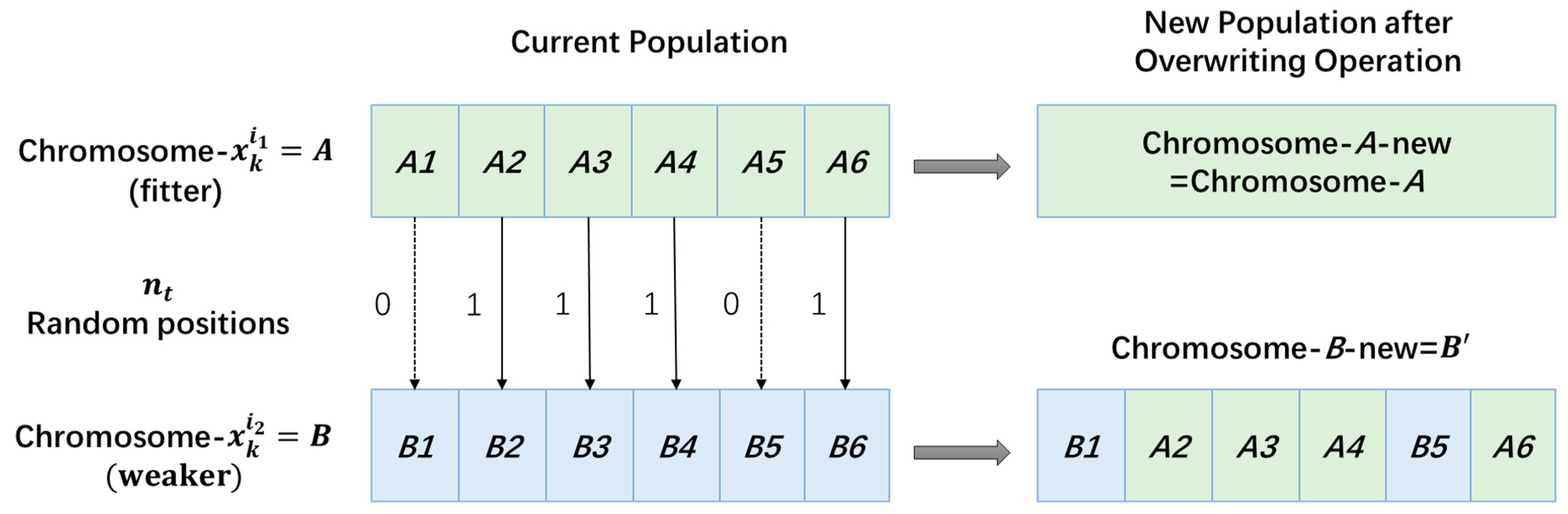
Here, in place of the conventional selection and crossover operators of a GA, an overwriting operator is implemented in the LPF on Lamarckian inheritance. This operator ensures that fitter organisms are given the priority directly to pass on their characteristics to their offspring in evolution. Suppose that each of the $N$ particles at time $k$, $x_k^i$, consists of six parameters of the RUL model as shown in Equation (2). Each parameter is termed a “phenotype” of “genes”. For simplicity of illustration, we assume that each parameter is represented by one gene. A complete set of the genes representing the parameter set is termed a “chromosome”. Consider two chromosomes at time k, $x_k^{i_1}=A=\left(A_1, A_2,A_3,A_4,A_5,A_6\right)$ and $x_k^{i_2}=B=\left(B_1, B_2,B_3,B_4,B_5,B_6\right)$, where $A$ is better than $B$, i.e., $fitness\left(A\right)>fitness\left(B\right)$.

In an LPF, for chromosomes $A$ and $B$ to produce offspring, a certain percentage of the genes of chromosome $B$ will be overwritten by corresponding genes of chromosome $A$, forming chromosome $B^{\prime }$ as a new candidate PF. The percentage of the overwriting genes transferred over to $B^{\prime }$ is termed the Lamarckian probability, which is denoted $p_t$ and is calculated as:

$$p_t=\left(\frac{fitness\left(A\right)}{fitness\left(B\right)+fitness\left(A\right)}\right)\%,$$

(10)

The numbers of genes transferred, $n_{\mathrm{t}}$, is calculated by:

$$n_{\mathrm{t}}=n_x·p_{\mathrm{t}},$$

(11)

where $n_x$ is the number of parameters (or genes in this simplified example) or the number of dimensions of a particle in the PF. This overwriting operation is depicted in Figure 1.

Hence, the number of genes passed on at crossover depends on the relative fitness of the two parental chromosomes. In this way, even if the fitness of chromosome B is too low, it will retain a small portion of its genes instead of being unselected as in a GA, thereby maintaining a degree of diversity in the gene pool and thus mitigating the particle impoverishment problem.

Further, the overwriting operation saves the mutation operation of a GA. With elitism, the overwriting operations will retain the best characteristics in the PF, while some lightweight particles are still present in the population for particle diversity potentially useful for future explorations.

3.2.3. Implementation of the LPF Algorithm

The steps of the LPF for RUL are given below.

Step 1: Initialization

Generate an initialization particle set $\left\{x_0^i\right\}, i=1,2,\cdots ,N$, by drawing from an assumed or a priori probability density $p\left(x_0\right)$. In the population, each particle or chromosome can be encoded in binary if necessary or if the number of parameters is relatively small, to explore finer estimation.

Step 2: Importance Sampling to Form an Initial Population

Sample $N$ particles with weights ${\left\{x_k^i,w_k^i\right\}}_{i=1}^N$ using the transition density $q$ $\left(x_k^i|x_{k-1}^i,z_k\right)=p\left(x_k^i|x_{k-1}^i\right)$ as the importance density to estimate the weight of each particle:

$${\tilde{w}}_k^i\propto {\tilde{w}}_{k-1}^i\frac{p(z_k|X_k^i)p(X_k^i|\left(X_{k-1}^i\right)}{q(X_k^i|\left(X_{k-1}^i,Z_k\right)},$$

(12)

for normalization to

$$w_k^i={\tilde{w}}_k^i/{{\displaystyle \sum }}_{i=1}^N{\tilde{w}}_k^i,$$

(13)

The importance sampling particle set ${\left\{x_k^i\right\}}_{i=1}^N$ at $k=0$ forms the initial population of the PF. The size of the population means the number of particles, which remains as $N$, constant to $k$ in the filtering process.

Step 3: Overwriting Operation

First, the overwriting chromosome is chosen according to the given inheritance probability. For instance, suppose that particles $i_1$ and $i_2$ are chosen with $w_k^{i_1}>w_k^{i_2}$. Then, the probability of each gene in $i_1$ to overwrite its corresponding gene in $i_2$ is calculated as:

$$p_t=\left(\frac{w_k^{i_1}}{w_k^{i_1}+w_k^{i_2}}\right)\%,$$

(14)

The numbers of genes transferred, $n_t$, is calculated by (11).

In this way, the lower-weight particle is overwritten in part by the higher-weight one with favorable genes, like gene editing in biochemistry. If the weight of one selected particle is zero, overwriting will not be performed. Note that the overwriting operation will automatically retain the elitist particle, as depicted in Figure 1. Hence, the LPF is always an elitism algorithm, as there is no need to use a mutation operation in an LPF.

Step 4: Evolution Until Termination

The particle set evolves generation by generation until the process terminates when a fixed number of iterations have been reached or no meaningful improvements may be obtained.

Step 5: Outputting the State Estimates

Then, the particle phenotypes are decoded back to real numbers of the optimal particles with equal weights ${\left\{{\tilde{x}}_k^i,1/N\right\}}_{i=1}^N$. By Equation (9), the system state is thus estimated as:

$$x_k=\frac{1}{N}{{\displaystyle \sum }}_{i=1}^N{\tilde{x}}_k^i,$$

(15)

3.2.4. State Updating and Prediction in the LPF Algorithm

The accurate estimation of battery capacity not only depends on a degradation model, but also on its parameters. According to [30], using the LPF, the estimated capacity for each particle at cycle $k$ is given by:

$$Q_k^i=a_k^i·exp\left(b_k^i·k\right)+c_k^i·exp\left(d_k^i·k\right),$$

(16)

and hence the capacity is estimated as:

$$Q_k={{\displaystyle \sum }}_{i=1}^N{w}_k^i·Q_k^i,$$

(17)

An $L$-step-ahead prediction at cycle $k$ with present observations can be estimated as:

$$Q_{k+L}^i=a_k^i·exp\left(b_k^i·\left(k+L\right)\right)+c_k^i·exp\left(d_k^i·\left(k+L\right)\right),$$

(18)

The estimated posterior PDF can be predicted at each trajectory with weights:

$$P(Q_{k+L}|Q_{0:k})\approx {{\displaystyle \sum }}_{i=1}^N{w}_k^i\delta \left(Q_{k+L}-Q_{k+L}^i\right),$$

(19)

Hence, the expectation of the L-step-ahead prediction yields:

$${\overline{Q}}_{k+L}={{\displaystyle \sum }}_{i=1}^N{w}_k^i{Q}_{k+L}^i,$$

(20)

As the failure threshold is 70% of the rated capacity, the RUL estimation $L_k^i$ of the ith trajectory is obtained by solving the equation:

$$a_k^{i}exp\left(b_k^i\left(k+L_k^i\right)\right)+c_k^{i}exp\left(d_k^i\left(k+L_k^i\right)\right)=0.7Q_{rated},$$

(21)

Then, the distribution of RUL is estimated as:

$$P(L_k|Q_{0:k})\approx {{\displaystyle \sum }}_{i=1}^N{w}_k^i\delta \left(L_k-L_k^i\right),$$

(22)

The expectation of the RUL at the cycle k is thus predicted as:

$${\overline{L}}_k={{\displaystyle \sum }}_{i=1}^N{w}_k^i{L}_k^i,$$

(23)

4. Experiments and Validation

Here, the performances of LPF is demonstrated in a single-dimensional (1D) system against the PF that is based on genetic algorithm with elitism (GAe), which is termed GAePF. The LPF is then compared with the standard PF for lithium-ion RUL prediction.

4.1. Single-Dimension Experiment

A nonlinear 1D experiment widely used in PF testing is given by [35]:

$$x_k=1+\sin \left(\alpha \pi k\right)+{\varnothing }_1{x}_{k-1}+v_k,$$

(24)

$$z_k=\{\begin{array}{cc}{\varnothing }_2{x}_k^2+r_k& k\le 30\\ {\varnothing }_3{x}_k-2+r_k& k>30\end{array},$$

(25)

where $v_k$ is a random variable modeling the process noise in Gamma(3,2); $\alpha =4\times {10}^{-2}$, ${\varnothing }_1={\varnothing }_3=0.5$, and ${\varnothing }_2=0.2$ are scalar parameters in the output model; and the observation noise is $r_k$, drawn from a Gaussian distribution $N\left(0, 0.00001\right)$. Different filters are used to estimate the state $x_k$ for $k=1,2,\dots ,T$, where the total observation time is $T=70$. The maximum number of generations is $G=20$. In the LPF, the inheritance probability is $\rho =0.5$. In the GAePF, the crossover probability and the mutation probability are 0.5 and 0.1, respectively. All of the PFs have $N=100$ particles. The experiment was carried out on Monte Carlo simulations with $M=200$.

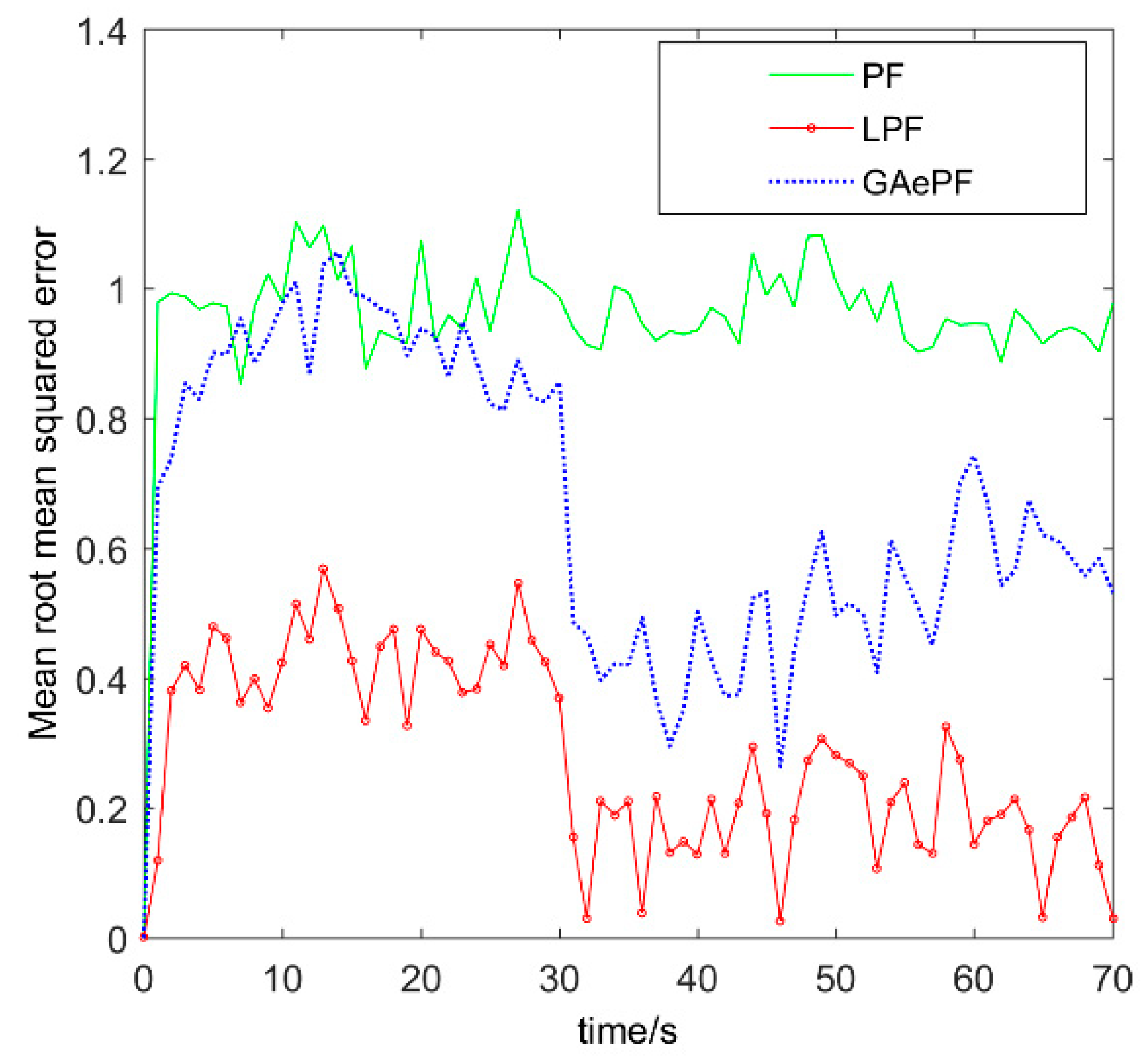
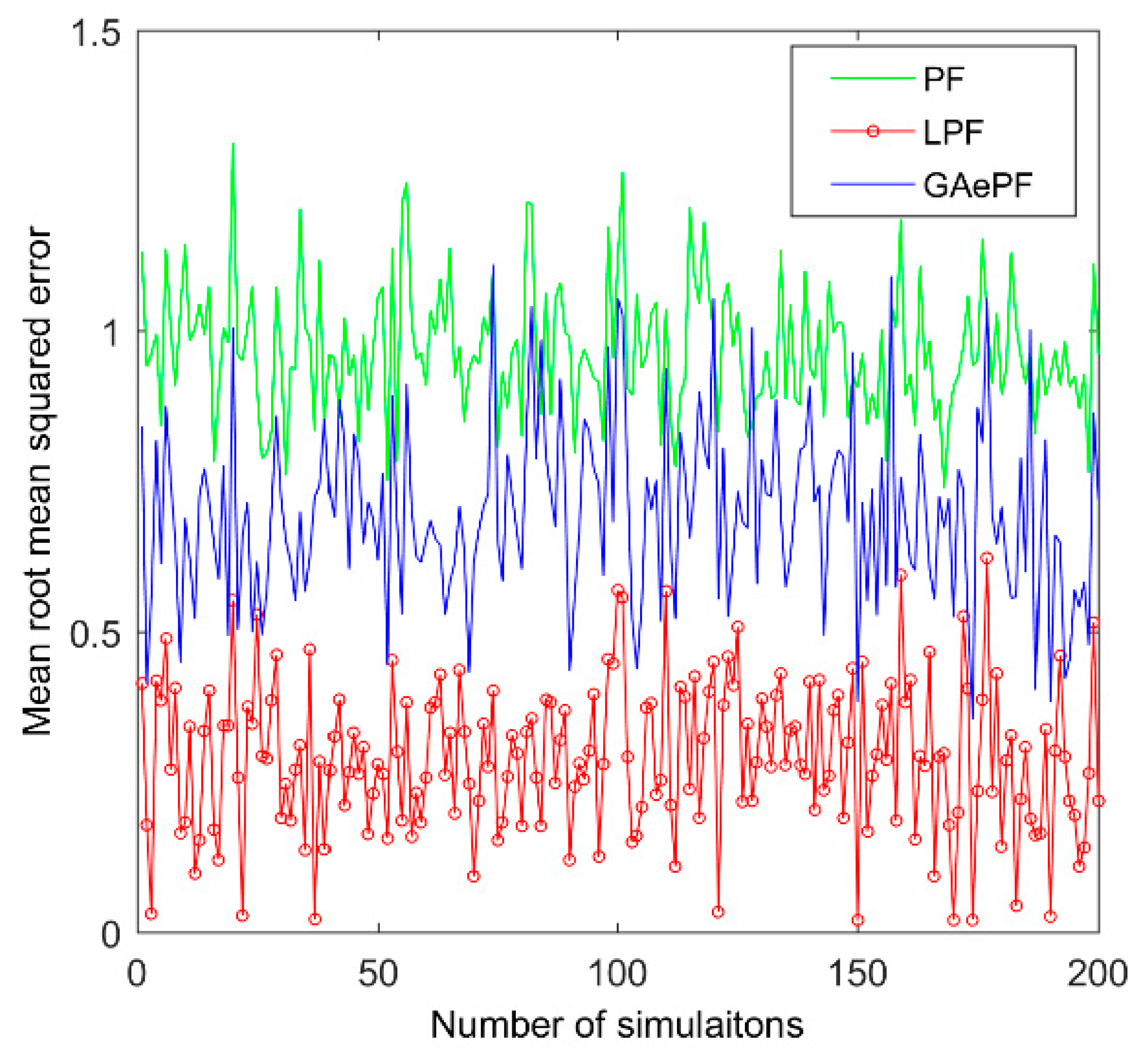
To evaluate the performance of LPF and GAePF, three root-mean-squared errors are used:

$$rmse=\sqrt{\frac{1}{T}{{\displaystyle \sum }}_{k=1}^T{\left(x_k-{\widehat{x}}_k\right)}^2},$$

(26)

$$\overline{rmse}=\sqrt{\frac{1}{M}{{\displaystyle \sum }}_{m=1}^M\left[\frac{1}{T}{{\displaystyle \sum }}_{k=1}^T{\left(x_k^m-{\widehat{x}}_k^m\right)}^2\right]},$$

(27)

$$rms{e}^{\prime }=\sqrt{\frac{1}{M}{{\displaystyle \sum }}_{m=1}^M{\left(x_k^m-{\widehat{x}}_k^m\right)}^2},$$

(28)

where the mean of $rmse$ is $\overline{rmse}$, $rms{e}^{’}$ is the $rmse$ for M simulations, $x_k^m$ the real state at time $k$ for the $m$th simulation, and ${\widehat{x}}_k^m$ the estimated state.

The mean estimation $rmse$ values of the generic PF, LPF, and GAePF for 200 simulations are presented in Figure 2 and Figure 3, respectively. As can be seen from the figures, the $rmse$ of the LPF is lower than that of the other two algorithms. The root mean square error $\left(rmse\right)$ results of the three algorithms with $N=100$ and $200$ are compared in

Table 1. Mean Root Mean Squared Error and Stop Time.

Algorithm	Performance Metrics
	Mean Root Mean Squared Error	Stop Time	N
PF	0.9604	0.2542	100
GAePF	0.8019	1.5454
PF	0.7604	0.6692	200
GAePF	0.6960	3.1651
LPF	0.2902	2.1539	100

. It can be seen that the estimation accuracy of the LPF with just 100 particles is better than that of the other two filters with 200 particles. In other words, the LPF not only improves the accuracy, but also has a higher utilization rate, while its runtime is close to that of the GAePF.

4.2. RUL Prediction for Lithium-Ion Battery

4.2.1. Experimental Battery Datasets

In this subsection, the proposed LPF framework for RUL prediction is validated against lithium-ion battery data provided by the NASA Ames Research Center Prognostics Center of Excellence [36]. The data were obtained at room temperature (24 °C).

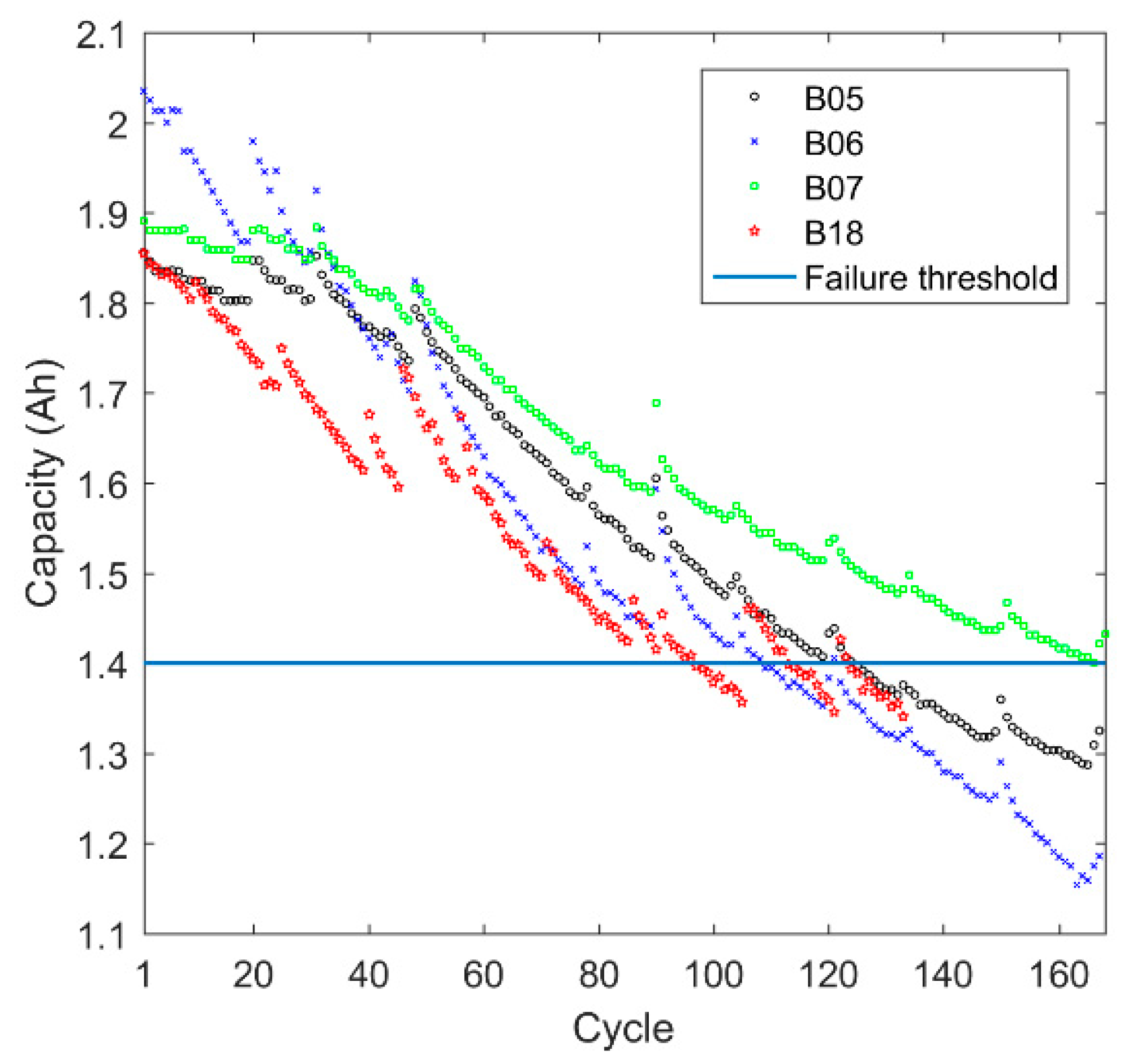
The dataset contains four cells, labeled as B05, B06, B07, and B18. Their nominal capacity is 2000 mAh, while the nominal voltage is 3.7 V. To estimate accelerated aging, multiple charge-discharge cycles were undertaken. All of the test cells went through the same constant-current (CC) and constant-voltage (CV) charging with current maintained at 1.5 A until the voltage reaches the upper limit of 4.2 V and then maintained until the current dropped to 20 mA. Similarly, discharging went through a constant current of 2 A until the voltages fell to 2.7 V, 2.5 V, 2.2 V, and 2.5 V for battery B05, B06, B07, and B18, respectively. The failure threshold was 1400 mAh.

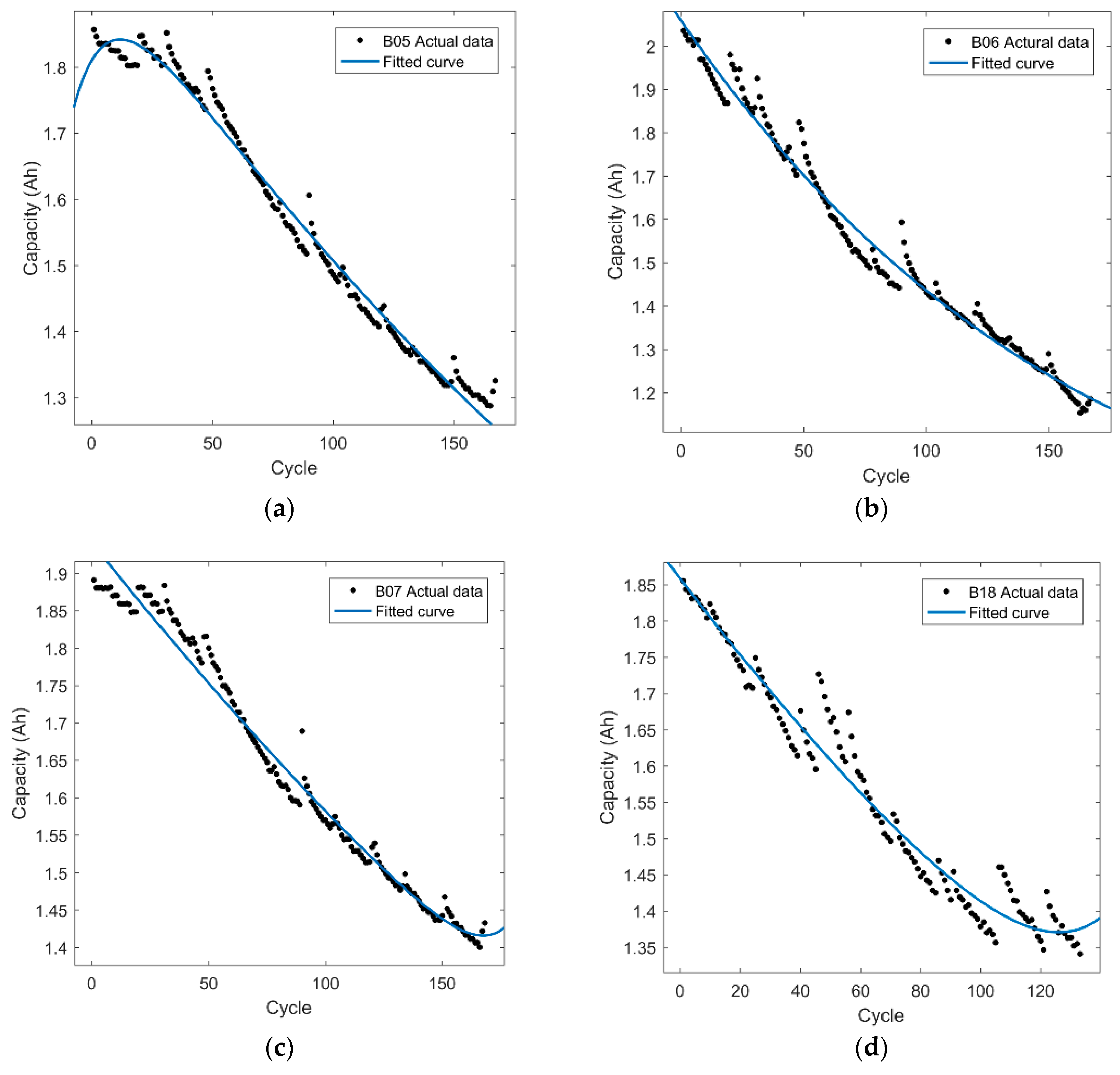
The capacity degradation trend is shown in Figure 4, where the degradation data were drawn using MATLAB^®®® (MathWorks, Natick, MA, USA) curve fitting. It can be seen that the empirical model of Equation (4) fit the regression process. Figure 5 shows that if the parameters are accurately estimated, the model fits the degradation trend.

To test the prediction accuracy, the data of batteries labeled B05, B06 and B07 were used as the training data. For validation, battery B18 was predicted using the LPF. For simplicity in this experiment, μ was set to 0.6 and ${\sigma }_a=1\times {10}^{-4}$, ${\sigma }_b=1\times {10}^{-6}$, ${\sigma }_c=1\times {10}^{-6}$, ${\sigma }_d=1\times {10}^{-7}$, and ${\sigma }_n=1\times {10}^{-3}$ for the Gaussian noise mode. Hence, only the four parameters $a$, $b$, $c$, and $d$ must be estimated in a particle. The parameters of the three known batteries were produced by the fitting to obtain initial training data, as shown in

Table 2. Model Parameters of Batteries and State Initialization.

Battery ID	State Variables	Initial Value	Fitting Range
B05	a	1.983	(1.963, 2.004)
	b	−0.002746	(−0.002838, −0.002654)
	c	−0.1738	(−0.2006, −0.1469)
	d	−0.06751	(−0.09014, −0.04488)
B06	a	1.579	(−1.745, 4.903)
	b	−0.00549	(−0.01438, 0.003402)
	c	0.4797	(−2.859, 3.819)
	d	0.0008834	(−0.01656, 0.01833)
B07	a	1.942	(1.933, 1.951)
	b	−0.002052	(−0.002126, −0.001978)
	c	1.572 × 10−7	(−2.198 × 10−6, 2.513 × 10−6)
	d	0.07406	(−0.01613, 0.1643)
Mean	a	1.8347	-
	b	−0.003429	-
	c	0.101967	-
	d	0.0024778	-

.

4.2.2. Results and Analysis

In this work, the initial parameters were set as their corresponding mean values of batteries B05, B06, and B07 shown in Table 2. The number of particles $N$ was set to 100. To test the robustness of the LPF method, different numbers of training cycles were used to compare the prediction results, which were the first 33 and 70 measurement cycles. To test the relative prediction performance, the results were compared with those obtained using the standard PF. Furthermore, the model accuracy was evaluated on the RUL absolute error (AE), the RUL relative prediction error (RPE), and the capacity root-mean-square-error (RMSE). These are defined as:

$$\mathrm{AE}=\left|{\mathrm{RUL}}_{\mathrm{true}}-{\mathrm{RUL}}_{\mathrm{prediction}}\right|,$$

(29)

$$\mathrm{RPE}=\mathrm{AE}/{\mathrm{RUL}}_{\mathrm{true}},$$

(30)

$$RMS{E}_{estimate}=\sqrt{\frac{1}{C}{{\displaystyle \sum }}_{k=1}^C\left(Q_k-\acute{Q_k}\right)},$$

(31)

$$RMS{E}_{prediction}=\sqrt{\frac{1}{Cp}{{\displaystyle \sum }}_{k=start}^C\left(Q_k-{\widehat{Q}}_k\right)},$$

(32)

where C is the number of measurement cycles, ${\acute{Q}}_k$ is the estimate at cycle k, $Cp$ is the number of cycles that must be predicted, and ${\widehat{Q}}_k$ the prediction result at cycle k.

Prediction Performance Analysis

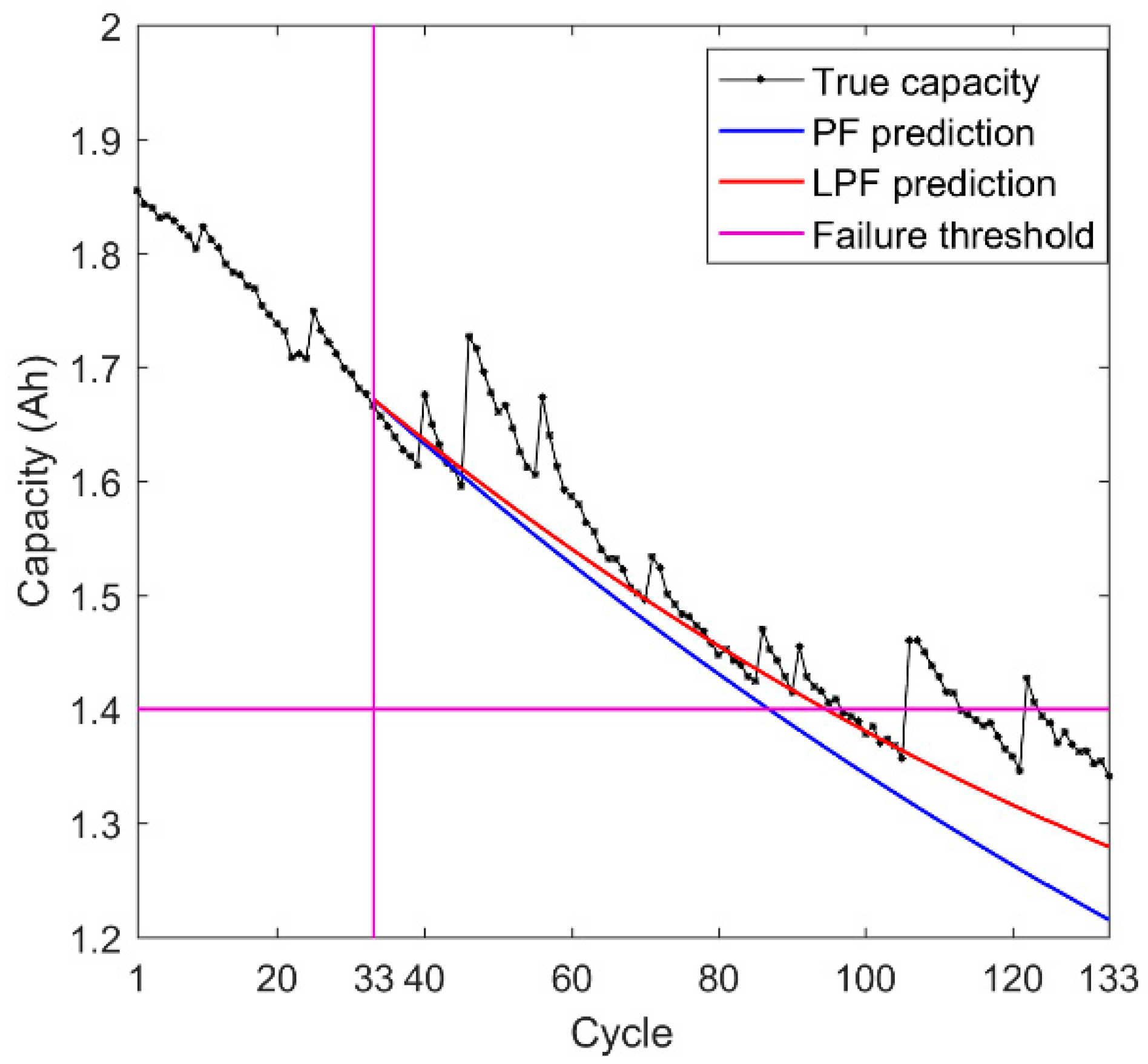
Figure 6 shows the RUL prediction results from the standard PF and the proposed LPF, where the first 33 cycles were used to update the prediction. Compared with the dataset, it is apparent that the LPF offers better predictions.

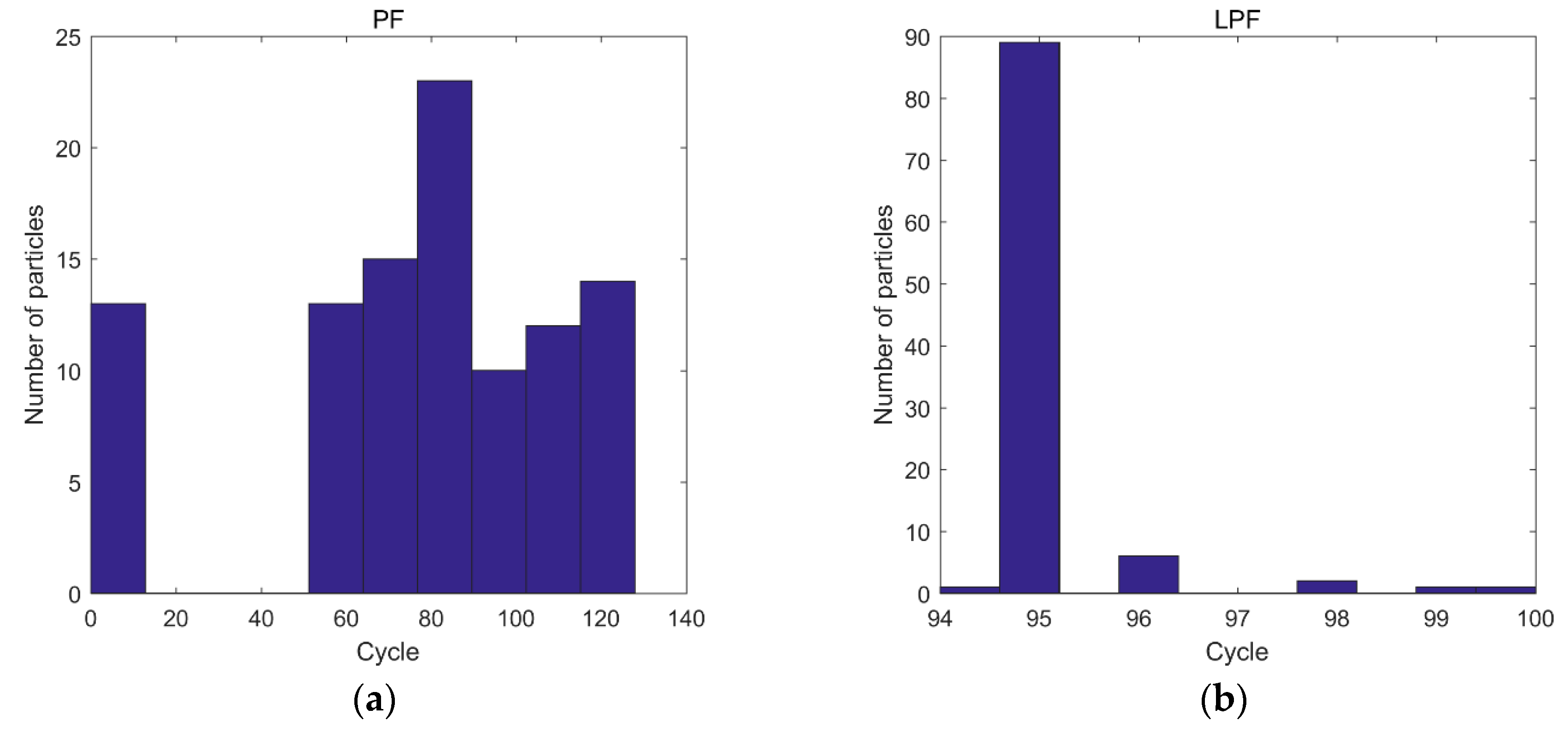
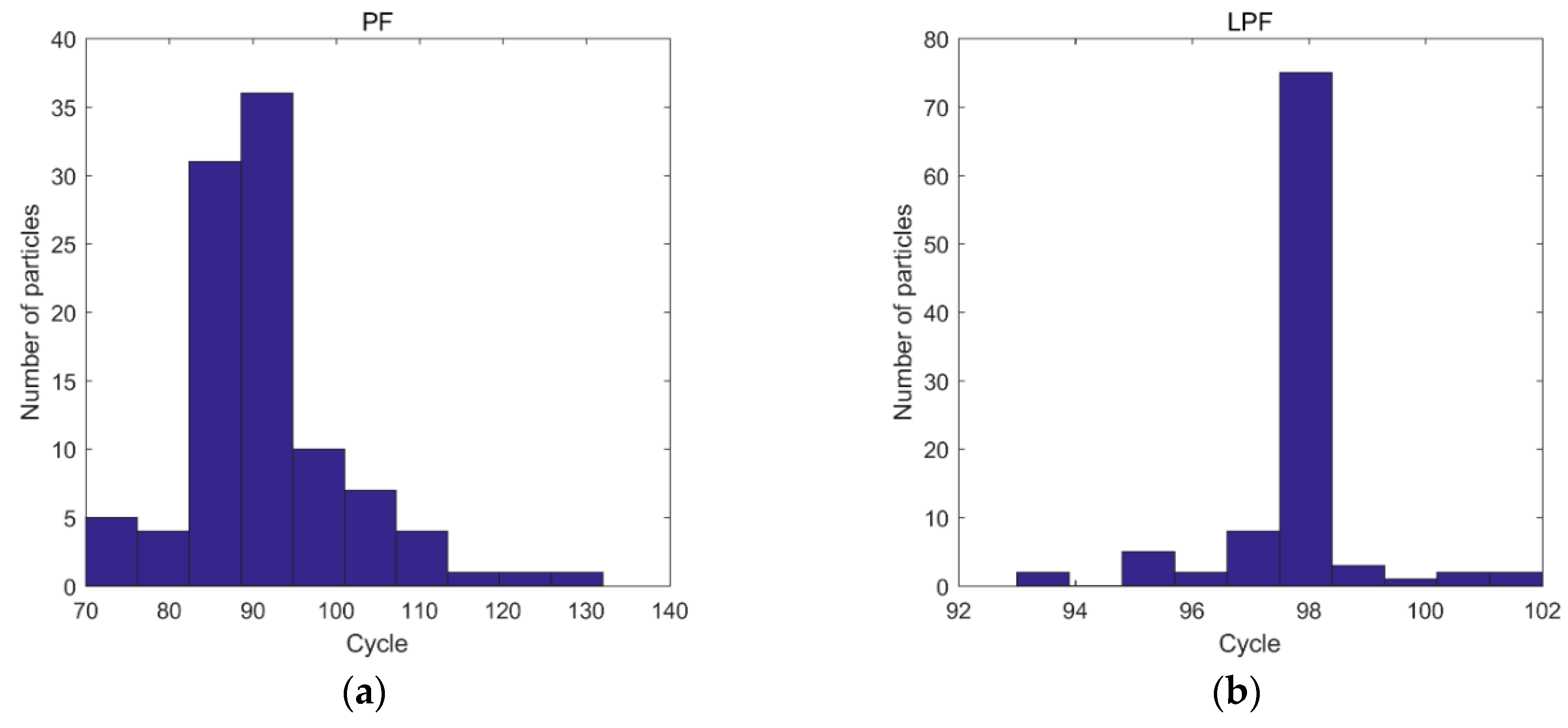
Figure 7 compares the histograms of the RULs predicted by the PF and LPF. It can be seen from Figure 7a that, using the PF method, more than 10% of the particles failed to predict the RUL from existing measurements during the first 33 cycles, and the estimated predicted RULs of cycles were within the range [50, 130], giving an average at 80 cycles, far away from the RUL data at 97 cycles. In contrast, Figure 7b plots the performance of the LPF predicted RULs within the range [94, 100], showing 90% of the particles predicting 95 cycles, which were very close to the true RUL of 97.

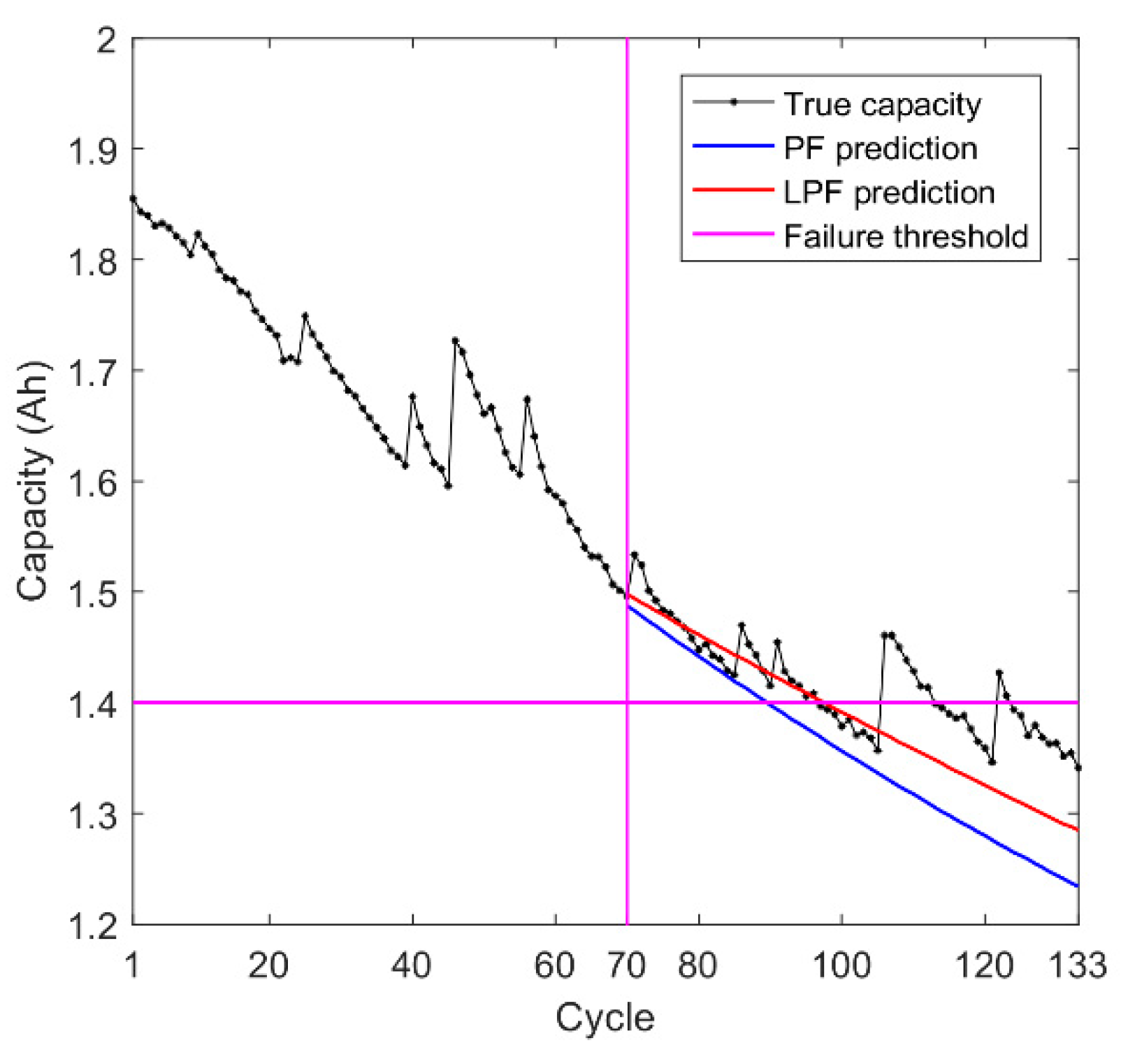
When using the first 70 cycles as measurement data to predict the RULs, Figure 8 similarly shows that the LPF offers better results. Figure 9a,b show the histograms of the RULs predicted by the PF and LPF, respectively. The same conclusions as drawn from Figure 6 and Figure 7 can be drawn from Figure 9, confirming the robustness of the LPF method.

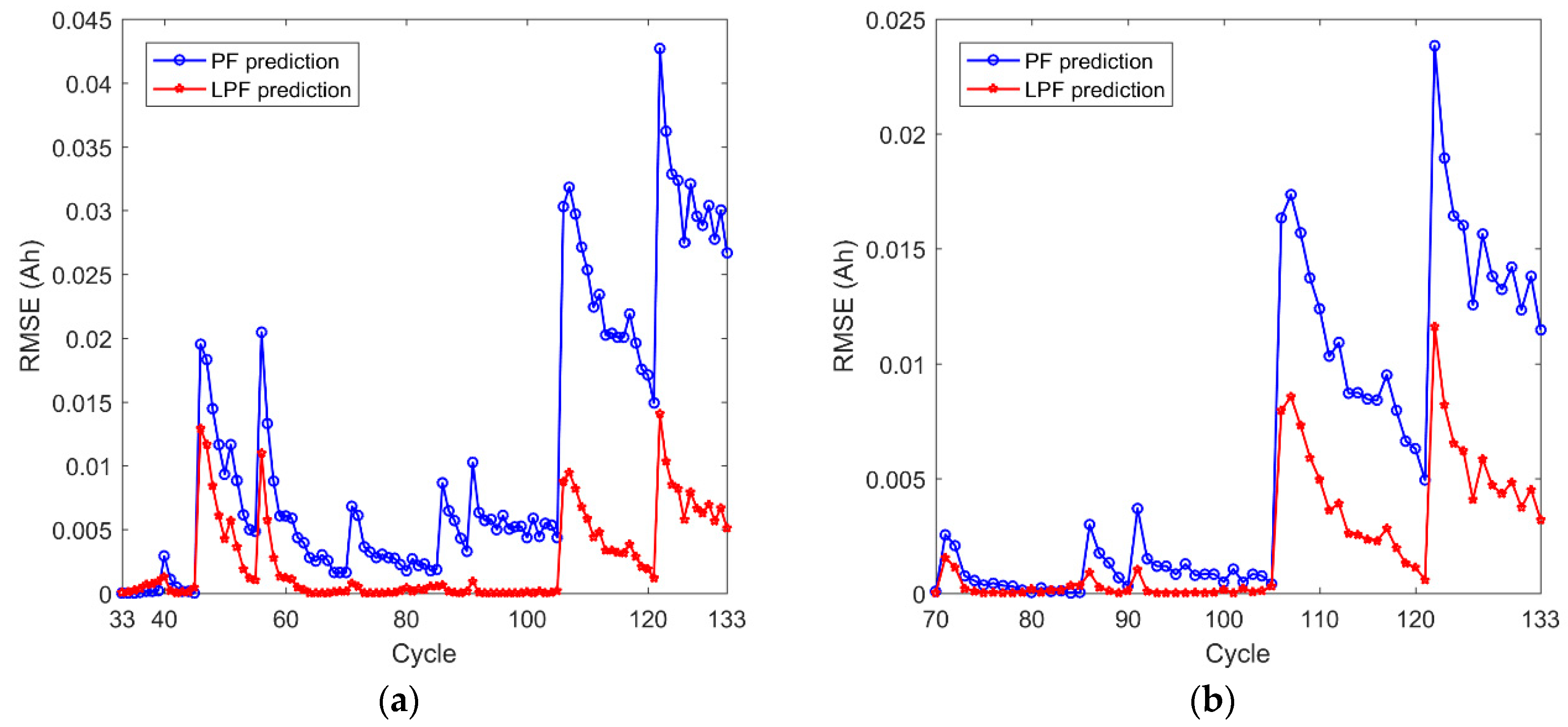
Figure 10a,b show the capacity RMSEs for the predictions using the PF and LPF methods, in which the first 33 and 70 cycles were used for the prediction, respectively. This confirms that the proposed LPF method results in a smaller RMSE than the PF.

Table 3. Prediction Results for Battery B18.

Cycles	True RUL	Algorithms	Prediction RUL	AE	RPE	RMSE
33	97	PF	87	10	10.3%	0.09084
		LPF	95	2	2.1%	0.04408
70		PF	90	7	7.2%	0.07705
		LPF	98	1	1%	0.04597

shows prediction errors between the two methods. It can be seen from the table that the predicted AEs, RPEs, and RMSEs obtained by the LPF are all smaller than those obtained with a standard PF.

One-Step Ahead Prediction Analysis

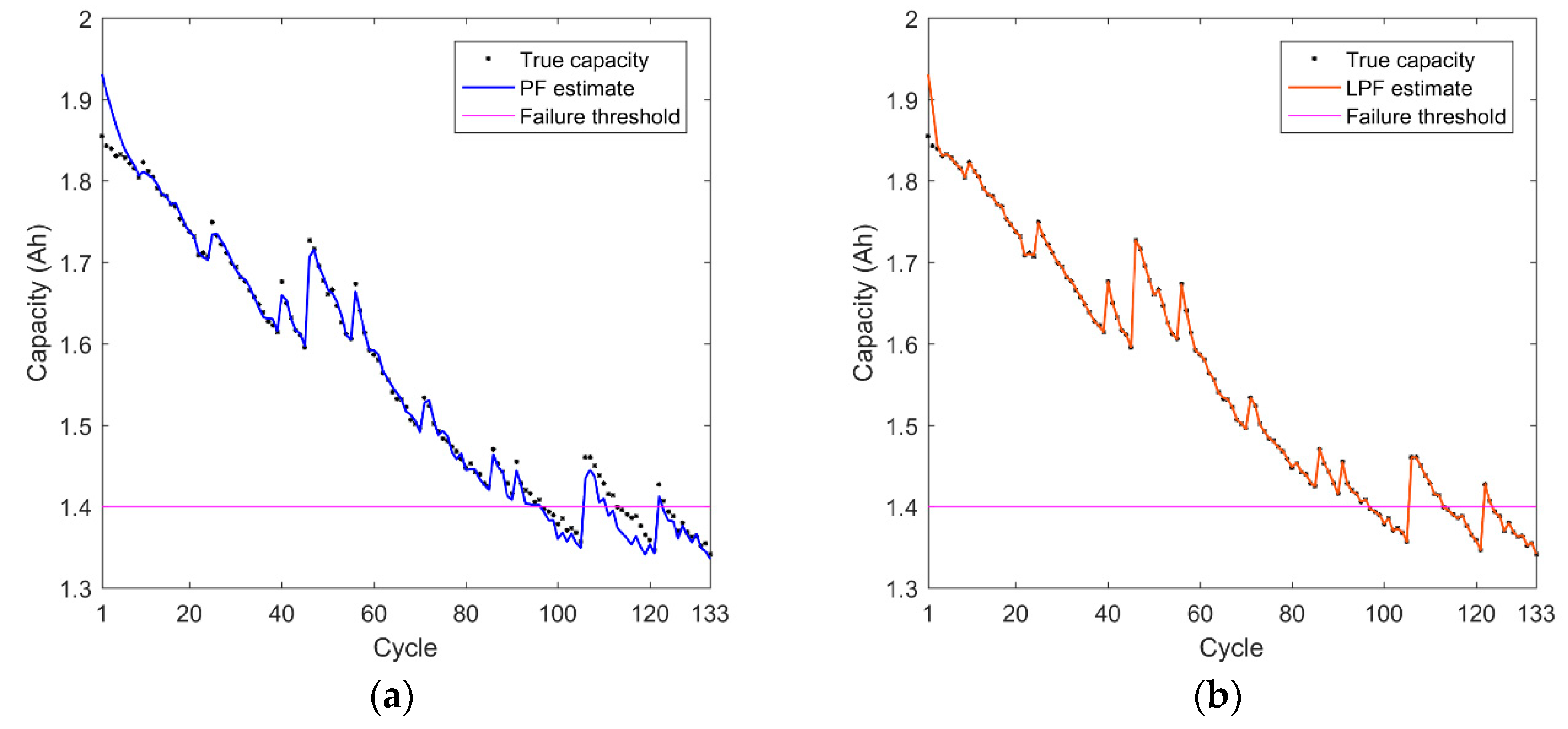
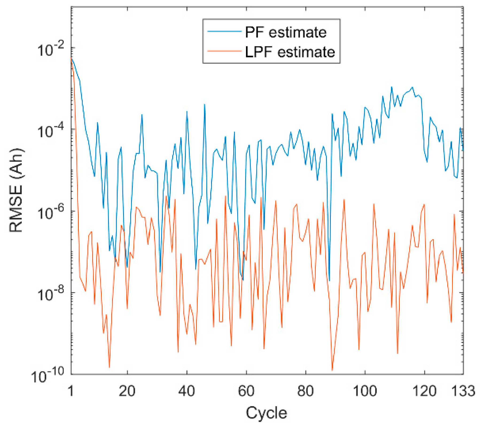
As all of the measurements of the battery could not be obtained while it was working, one-step prediction performance will also be considered as an on-line prediction reference. Figure 11a,b show the one-step-ahead capacity estimates using the standard PF and proposed LPF, respectively. Again, the LPF offers better results than the PF. To visualize the performance difference more clearly, the capacity RMSEs of the estimates at every cycle are compared in Figure 12 and mean RMSEs of all cycles are compared in

Table 4. Mean RMSE of One-Step-Ahead Capacity Estimates.

Algorithms	Mean RMSE (Ah)
PF	0.01098
LPF	0.00706

. The results of these comparisons confirm that the LPF is a better method.

5. Conclusions

In this work, a novel approach to predicting lithium-ion battery’s remaining useful life has been developed and evaluated. In the literature, effective forecast of remaining useful life has been reported using a particle filter, but it suffers from particle degeneracy and impoverishment deficiencies. The Lamarckian particle filter developed in this paper was to solve these problems for the first time to improve and broaden prediction of lithium-ion battery RUL.

Since the standard PF is a widely used algorithm for RUL prediction, we have used the RUL estimations from the traditional methods for comparison and have mapped a battery degradation model onto a particle filter problem. The LPF method developed in this paper is based on the PF estimates using the genetic algorithm framework with a Lamarckian inheritance mechanism. A Lamarckian inheritance operator has been developed to reduce particle degradation, enhance particle diversity and simplify the filtering process. Thus, the optimized particle will tend to cluster around the high likelihood region. The LPF has yielded better estimates of the RUL for cases considered with different numbers of measurement data, which are from NASA lithium-ion battery capacity degradation database, in terms of the average.

Moreover, according to histograms of the predicted RUL particle distribution using 33 and 70 observations, we draw the conclusion that more particles of the LPF when making a prediction were concentrated on the true RUL. In other words, the LPF well overcomes the lack of the particle collapsing problem, resulting in particle degeneracy and impoverishment. Further, better prediction results can be obtained using one-step ahead LPF prediction when the charge and discharge cycles proceed. This indicates that the proposed method has a good adaptability for lithium-ion battery degradation with non-linear and non-Gaussian characteristics.

It is expected that the LPF method can cope with more complex RUL models. Hence, in planned future research, the LPF method will be used to improve the underlying RUL model itself, and to make the prediction self-adaptive.

References

- Yu, Z.; Xiao, L.; Li, H.; Zhu, X.; Huai, R. Model parameter identification for lithium batteries using the coevolutionary particle swarm optimization method. IEEE Trans. Ind. Electron. 2017, 64, 5690–5700. [Google Scholar] [CrossRef]
- Dong, G.; Wei, J.; Chen, Z. Kalman filter for onboard state of charge estimation and peak power capability analysis of lithium-ion batteries. J. Power Sources 2016, 328, 615–626. [Google Scholar] [CrossRef]
- Kim, I.L.S. A technique for estimating the state of health of lithium batteries through a dual-sliding-mode observer. IEEE Trans. Power Electron. 2010, 25, 1013–1022. [Google Scholar]
- Wu, J.; Wang, Y.; Zhang, X.; Chen, Z. A novel state of health estimation method of Li-ion battery using group method of data handling. J. Power Sources 2016, 327, 457–464. [Google Scholar] [CrossRef]
- Xiong, R.; Yu, Q.; Shen, W.; Lin, C.; Sun, F. A sensor fault diagnosis method for a lithium-ion battery pack in electric vehicles. IEEE Trans. Power Electron. 2019, 34, 9709–9718. [Google Scholar] [CrossRef]
- Barrera, J.; Galeano, N.; Maldonado, H. SoC estimation for lithium-ion batteries: Review and future challenges. Electronics 2017, 6, 102. [Google Scholar] [CrossRef]
- Dong, G.; Chen, Z.; Wei, J.; Ling, Q. Battery health prognosis using Brownian motion modeling and particle filtering. IEEE Trans. Ind. Electron. 2018, 65, 8646–8655. [Google Scholar] [CrossRef]
- Mejdoubi, A.; Oukaour, A.; Chaoi, H.; Gualous, H.; Sabor, J.; Slamani, Y. State-of-charge and state-of-health lithium-ion batteries diagnosis according to surface temperature variation. IEEE Trans. Ind. Electron. 2016, 63, 2391–2402. [Google Scholar] [CrossRef]
- Eddahech, A.; Briat, O.; Bertrand, N.; Delétage, J.-Y.; Vinassa, J.-M. Behavior and state-of-health monitoring of Li-ion batteries using impedance spectroscopy and recurrent neural networks. Int. J. Elect. Power Energy Syst. 2012, 42, 487–494. [Google Scholar] [CrossRef]
- Liu, D.; Zhou, J.; Pan, D.; Peng, Y.; Peng, X. Lithium-ion battery remaining useful life estimation with an optimized relevance vector machine algorithm with incremental learning. Measurement 2015, 63, 143–151. [Google Scholar] [CrossRef]
- Liu, D.; Yin, X.; Song, Y.; Liu, W.; Peng, Y. An on-line state of health estimation of lithium-ion battery using unscented particle filter. IEEE Access 2018, 6, 40990–41001. [Google Scholar] [CrossRef]
- Kim, J.; Cho, B.-H. State-of-charge estimation and state-of-health prediction of a li-ion degraded battery based on an EKF combined with a per-unit system. IEEE Trans. Veh. Technol. 2011, 60, 4249–4260. [Google Scholar] [CrossRef]
- Chen, Z.P.; Wang, Q.T. The application of UKF algorithm for 18650-type lithium battery SOH estimation. Appl. Mech. Mater. 2014, 519–520, 1079–1084. [Google Scholar] [CrossRef]
- Hu, C.; Youn, B.D.; Chung, J. A multiscale framework with extended Kalman filter for lithium-ion battery SOC and capacity estimation. Appl. Energy 2012, 92, 694–704. [Google Scholar] [CrossRef]
- Zheng, X.; Fang, H. An integrated unscented kalman filter and relevance vector regression approach for lithium-ion battery remaining useful life and short-term capacity prediction. Reliab. Eng. Syst. Saf. 2015, 144, 74–82. [Google Scholar] [CrossRef]
- Liu, S.-L.; Cui, N.-X.; Zhang, C.-H. State of health estimation of lithium-ion battery based on AUKF. Power Electron. 2017, 11, 122–124. [Google Scholar]
- Banerjee, A.; Burlina, P. Efficient particle filtering via sparse kernel density estimation. IEEE Trans. Image Process. 2010, 19, 2480–2490. [Google Scholar] [CrossRef] [PubMed]
- Gordon, N.; Salmond, D.; Smith, A. Novel approach to nonlinear/non-Gaussian Bayesian state estimation. IEEE Proc. F 1993, 140, 107–113. [Google Scholar] [CrossRef] [Green Version]
- Dong, G.; Chen, Z.; Wei, J.; Zhang, C.; Wang, P. An online model-based method for state of energy estimation of lithium-ion batteries using dual filters. J. Power Sources 2016, 301, 277–286. [Google Scholar] [CrossRef]
- Dalal, M.; Ma, J.; He, D. Lithium-ion battery life prognostic health management system using particle filtering framework. Proc. Mech. Eng. Part O J. Risk Reliab. 2011, 225, 81–90. [Google Scholar] [CrossRef] [Green Version]
- Liu, J.; Wang, W.; Ma, F. A regularized auxiliary particle filtering approach for system state estimation and battery life prediction. Smart Mater. Struct. 2011, 20, 075021. [Google Scholar] [CrossRef]
- Miao, Q.; Xie, L.; Cui, H.; Liang, W.; Pecht, M. Remaining useful life prediction of lithium-ion battery with unscented particle filter technique. Microelectron. Reliab. 2012, 53, 805–810. [Google Scholar] [CrossRef]
- Sbarufatti, C.; Corbetta, M.; Giglio, M.; Cadini, F. Adaptive prognosis of lithium-ion batteries based on the combination of particle filters and radial basis function neural networks. J. Power Sources 2017, 344, 128–140. [Google Scholar] [CrossRef]
- Wang, D.; Yang, F.; Tsui, K.L.; Zhou, Q.; Bae, S.J. Remaining useful life prediction of lithium-ion batteries based on spherical cubature particle filter. IEEE Trans. Instrum. Meas. 2016, 65, 1282–1291. [Google Scholar] [CrossRef]
- Zhang, X.; Miao, Q.; Liu, Z. Remaining useful life prediction of lithium-ion battery using an improved UPF method based on MCMC. Microelectron. Reliab. 2017, 75, 288–295. [Google Scholar] [CrossRef]
- Zou, G.H.; Jing, Z.L.; Hu, H.-T. Particle filter algorithm based on optimizing combination resampling. J. Shanghai Jiaotong Univ. 2016, 40, 1135–1139. [Google Scholar]
- Zhang, H.; Miao, Q.; Zhang, X.; Liu, Z. An improved unscented particle filter approach for lithium-ion battery remaining useful life prediction. Microelectron. Reliab. 2018, 81, 288–298. [Google Scholar] [CrossRef]
- Duong, P.; Raghavan, N. Heuristic Kalman optimized particle filter for remaining useful life prediction of lithium-ion battery. Microelectron. Reliab. 2018, 81, 232–243. [Google Scholar] [CrossRef]
- Tan, K.C.; Li, Y. Grey-box model identification via evolutionary computing. Control Eng. Pract. 2002, 10, 673–684. [Google Scholar] [CrossRef] [Green Version]
- He, W.; Williard, N.; Osterman, M.; Pecht, M. Prognostics of lithium-ion batteries based on Dempster–Shafer theory and the Bayesian Monte Carlo method. J. Power Sources 2011, 196, 10314–10321. [Google Scholar] [CrossRef]
- Yin, S.; Zhu, X. Intelligent Particle Filter and Its Application to Fault Detection of Nonlinear System. IEEE Trans. Ind. Electron. 2015, 62, 3852–3861. [Google Scholar] [CrossRef]
- Dawkins, R. The Blind Watchmaker: Why the Evidence of Evolution Reveals a Universe without Design; W.W. Norton & Co Inc.: New York, NY, USA, 1996. [Google Scholar]
- Brian, R. A Lamarckian Evolution Strategy for Genetic Algorithms. In The Practical Handbook of Genetic Algorithms; Chambers, L., Ed.; CRC Press: Boca Raton, FL, USA, 1999. [Google Scholar]
- Tan, K.C.; Li, Y. Performance-based control system design automation via evolutionary computing. Eng. Appl. Artif. Intell. 2001, 14, 473–486. [Google Scholar] [CrossRef] [Green Version]
- Wang, Y.; Sun, F.; Zhang, Y. Central difference particle filter applied to transfer alignment for SINS on missiles. IEEE Trans. Aerosp. Electron. Syst. 2012, 48, 375–387. [Google Scholar] [CrossRef]
- Saha, B.; Goebel, K. Battery Data Set. NASA Ames Prognostics Data Repository, NASA Ames Research Centre, Moffett Field, CA, USA. 2007. Available online: https://ti.arc.nasa.gov/tech/dash/groups/pcoe/prognostic-data-repository/ (accessed on 1 March 2019).
Figure 1.
Lamarckian particle filter (LPF) A and LPF B forming offspring B’ via overwriting operation.
Figure 2.
Mean root mean square error (rmse) with observation times for 200 simulations of three algorithms compared.
Figure 3.
Mean rmse with simulation numbers of three algorithms compared.
Figure 4.
NASA Ames Research Center Prognostics Center of Excellence battery dataset.
Figure 5.
Degradation data and fitting curves of the four batteries: (a) B05; (b) B06; (c) B07; (d) B18.
Figure 6.
Prediction comparison using 33 cycles for battery B18 of a remaining useful life (RUL) of 97 cycles.
Figure 7.
Histograms of predicted RUL distribution for battery B18, using 100 particles and 33 observations for the particle filter (PF) and the LPF methods: (a) PF; (b) LPF.
Figure 8.
Prediction comparison using 70 cycles for battery B18 of a RUL of 97 cycles.
Figure 9.
Histograms of predicted RUL distribution for battery B18, using 100 particles and 70 observations for the PF and the LPF methods: (a) PF; (b) LPF.
Figure 10.
Capacity RMSEs for PF and LPF predictions: (a) Using 33 cycles as measurements; (b) Using 70 cycles as measurements.
Figure 11.
One-step-ahead estimates of capacity degradation trends for battery B18: (a) PF; (b) LPF.
Figure 12.
Comparison of capacity estimate RMSEs for battery B18 between the PF and the LPF methods.