New Method for Calculating the Heating of the Conductor

1
SODO d.o.o., Minařikova ulica 5, SI-2000 Maribor, Slovenia
2
ELES d.o.o., Hajdrihova 2, SI-1000 Ljubljana, Slovenia
3
Faculty of Electrical Engineering, University of Maribor, Smetanova 17, SI-2000 Maribor, Slovenia
*
Author to whom correspondence should be addressed.
Energies 2019, 12(14), 2769; https://doi.org/10.3390/en12142769
Submission received: 17 June 2019
/
Revised: 8 July 2019
/
Accepted: 11 July 2019
/
Published: 18 July 2019
(This article belongs to the Section F: Electrical Engineering)
Abstract
:The paper describes the core heating of ACSR (aluminum conductor steel—reinforced) conductor in stable operation under different environmental conditions. The calculations are greatly simplified in a steady state—we can calculate on a balance of power instead of a balance of energies. At a known surface, the temperature of the conductor due to solar radiation, natural convection, and joules heating as well as the temperature of the steel core were calculated, which is relevant for the tensile strength of the rope. Measurements of the surface of the conductor and the core rejected a simple model of heat transfer—it is also necessary to take into account empty air spaces between the wires of a rope. On the basis of measurements, a new model has given satisfactory compliance with the measured values.
1. Introduction
In the design of distribution and transmission networks the choice of cross-section affects several factors such as a voltage drop, a power loss, stability, and protection. The temperature rise [1] of the conductors above the ambient temperature is important. It is necessary to know the largest continuous current of the conductor, since it determines the maximum allowed temperature of the conductor. The temperature of the conductor affects the sag of the conductor between the pillars and determines the change in the tensile strength due to heating [2,3,4,5].
In calculating the load capacity of the conductors, attention must be paid primarily to the mechanical properties depending on the temperature [6,7,8].
Three temperatures are important: Joule heating [9] depends on the average conductor temperature, and natural convection [10] and radiation depend on the surface temperature of the conductor [11,12,13]. The change in the tensile strength in the first approximation depends on the temperature of the strands of the rope in the middle of the conductor.
In the articles [14,15,16], a sensitivity analysis was performed based on operating conditions (wind, solar, current) [14,15,16] and on the IEEE standard [17] for calculating the temperature of the conductor. In the article [13], a current is determined based on the calculation and measurement of the average temperature of the conductor [18].
It was also emphasized that, under exceptional conditions, the thermal creep and the loss of tensile strength of the conductor must be taken into account [15,19,20,21].
In this paper, a new method for calculating the warming of overhead lines (Al/Fe conductors) is presented.
Despite a good contact between the individual layers of aluminum, which is ensured at the time of manufacture, there is a great deal of influence between the empty spaces between the wires. If they are ignored, the rope has almost the same (thermal) properties as a homogeneous conductor, and the temperature in the axis is almost equal to the temperature on the surface. Considering the empty spaces between the wires, the thermal conductivity is about a hundred times smaller. The differences between the surface and center temperatures are also greater.
The new method, which results from the surface temperature of the conductor and takes into account the empty spaces between the wires, was confirmed by measurements.
In the paper, individual influencing factors on the conductor are shown, consequently indicating whether they heat it or cool it in a stable operation. In the second chapter, a general thermal equation of conductors has been written. In the third chapter, the simplification of the general equation for stable operation with emphasis on radiation, natural convection, and electric heating, is presented.
In the fourth chapter, the increase in temperature from the layers from the surface to the interior was determined. In the fifth chapter, the measurements that were rejected by the simple ACSR model of the conductor in the fourth chapter, are described. In the sixth chapter, in the conductor model, the empty spaces between the wires of the individual layers were taken into account, and the measured results confirmed the results. This is also confirmed by the new method of calculating the heating of the conductors.
2. Selection of Cross Section of the Conductors Considering on Heating
Each conductor is heated if an electric current flows through it. If all the heat produced in the conductor was consumed for heating, the temperature of the conductor would rise steadily. When the temperature of the conductor rises above the ambient temperature, the conductor sends the heat into the surroundings.
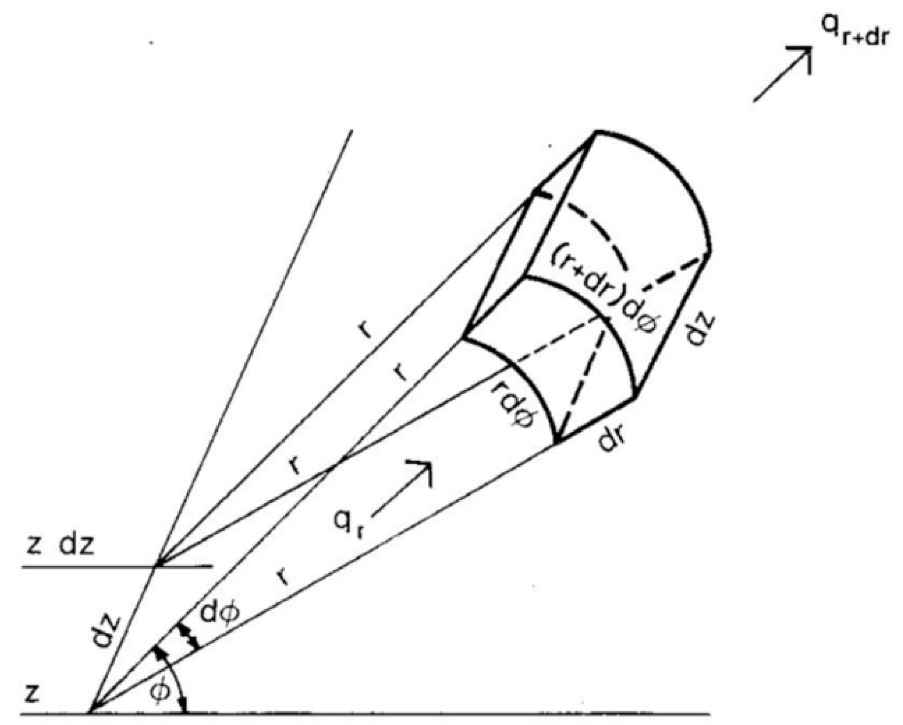
Figure 1 shows the flow of heat in the elemental volume with the indicated geometric and material parameters.
General thermal equation of conductors (1) after V. T. Morgan [22]:
where Q(T) is temperature-dependent heat produced per unit volume, λ(T) is temperature-dependent thermal conductivity, γ is specific weight, c is specific heat, T is temperature, and r, z, φ are geometric parameters.
3. Stabile Operation
In stable operation, there are events observed—energy in a time unit, that is, power. All energy equilibrium is simplified in the balance of power. For reasons of transparency, the fact that the conductor can be hidden a few meters from the sun so the heat flow is not observed in the longitudinal direction (z-axis) is not taken into account. Given the fact that the factors of immission and emissivity for clear, cloudy skies, grassy surfaces and fields are not known, both the emissivity and the albedo are set up by the same one, thus obtaining a rotational symmetric system [23].
3.1. Power of Radiation
In the case of heating the conductor, a comparison between the calculated values with the new method and during the measurements was made.
Figure 2 shows the conductor we are exploring and on which we performed the measurements described below in the article.
Using (2), the amount of light that irradiates a 1 m long piece of the conductor at temperature T = 20 °C = 293 K was calculated. For reasons of transparency it is supposed that the surface is ideally black.
where P means light current, Sv is surface of the conductor [m2], Sv = 2·π·r·1 m = 2·π·0.0153 m·1 m = 0.096 m2, φ is density of radiation flow of the black body, σ is a universal constant, known as Štefan–Boltzmann constant, T is temperature.
Because the rope conductor loses 40 J at a temperature of 20 °C per second, under these circumstances, it would be cooled every second for (P/(m·cp·dT) = 40/1547) = 0.026 K.
Bodies around the rope also have the same temperature (20 °C) and are not ideally black. The rope from the surroundings gets exactly the same amount of energy, namely
When the sun shines on the conductor, the light flux is joined by the previous 40 watts:
where φs is a solar constant (1000 W/m2).
As an irradiated surface, due to the curvature, the longitudinal cross-section Ap = 2·r·1 = 2·0.0153 m·1 m = 0.0306 m2 is taken. The conductor reaches such a T temperature to transmit exactly as much energy per second as it receives. If only the light currents are considered, the balance is the following:
where φs is solar energy density at surface [W/m2], Ap is longitudinal section of the conductor [m2], σ is Štefan–Boltzmann’s constant 5.68 × 10⁸ W/(m2 K4), T0 is ambient temperature [K], Tp is surface temperature of the conductor [K], Sv is surface of the conductor [m2].
Considering the solar constant (E0 = 1367 W/m2) less for passing through the atmosphere (φs = 1000 W/m2), it is:
Figure 3 shows the heat flux in equilibrium.
3.2. Convection
Convection is the transition of heat from solid bodies to a gaseous (liquid) medium and vice versa [24].
The research of heat flows due to convection [25,26] gave the following empirical formulas for determining the size of these flows:
where α is thermal transfer coefficient [W/(m2 K)] (depending on the position and shape of the wall), Tp is the temperature of the convection surface [K], To is the temperature of the surrounding medium [K], S is surface [m2].
For a horizontal tube [27], the heat flux density can be calculated as follows:
Taking radiation and convection into account, the equilibrium equation for power is for Al/Fe 490/65 mm2 conductor per unit of length:
In this case, the markings are equal to (5) and additionally d is a pipe diameter (conductor) [m].
The equation is not algebraically solvable. With the numerical tangent method [28], the surface temperature of the conductor is 316 K. or 43 °C.
Assuming that the surface of the conductor is the ideal black body, it is heated in the sun to 65 °C, the convection (without wind) cools it to 43 °C (Figure 4).
3.3. Electric Heating
The amount of heat released is proportional to the square of the current (Joule’s law):
where Q is heat due to electric current, I is current of the conductor, R is resistance of the conductor, t is time, ρel is specific resistance and A is section of the conductor.
The resistance of the conductor depends on the shape and the substance forming the conductor, and furthermore from the temperature, frequency and current density flowing through the conductor [10].
Normally, at the ropes, in the calculations of operating states, only the resistance (conductivity) of the aluminum cover is considered. For the generality, the conductivity of the steel core and the proper distribution of the current along the layers [29] will also be taken into account. The maximum allowed current for the conductor Al/Fe 490/65 mm2 is 960 A.
The equilibrium equation, taking into account the current, is then:
In this case the marks are as in (5).
Using the tangent numerical method [28], the surface of the conductor is obtained 354 K or 81 °C.
Assuming that the surface of the conductor is the ideal black body, it is heated in the sun to 65 °C, the convection cools it to 43 °C, maximum allowable current I = 960 A heats it to 81 °C (Figure 5).
4. Heating a Conductor by Layers
In the case of electric conductors, mainly the steel core determines the tensile strength and thus the sag and spacing from the ground [21,30]. The change in the tensile strength in the first approximation depends on the temperature of the strands of the rope. Internal, warmer strands lose tensile strength faster, therefore, it is necessary to count or also measure the temperature gradient.
In the steady state, the temperature of the surface of the conductor was calculated. The basic equation for calculating the temperature of individual layers is the equation for the heat flux (power) through a differential thin wall [22]:
where P, PFe and PAl is electrical power at the appropriate temperature.
Through a differential thin tube (wall thickness dr) in time dt transfers heat flow Ф from the steel core (PFe) and a part of the heat flow from a source in aluminum to a radius r (Figure 6):
The temperature in the axis of the conductor can also be calculated (Figure 7).
where Ф is heat due to electric current, P, PFe and PAl is power or specific power, VFe and VAl is volume, r, rAl and rFe is radius, l is length, λAl and, λFe is specific conductivity, and Tp is surface temperature.
In Table 1, the temperatures are given as a function of the distance from/to the surface.
Despite of calculating the layers, the heat flow is the same as for a solid conductor.
5. Measurement of Current by Layers
In order to check the accuracy of the calculations in the previous chapter, the distribution of the current along the layers had to be checked first. At about 2 m long piece of the stranded conductor, about 10 cm of aluminum wires were removed in the middle (to gain access to the steel core) and the ‘peeled’ part of the rope only with the removed aluminum wires were shortened (Figure 8).
The results of the measurements were different from the expectations (Table 2).
The sum of the currents was in the class of accuracy of the clamp meters. In checking the matching of all three measured currents, it was found that the deviations were within the limits of the accuracy class of the clamp meters.
The expected current distribution at the total current 960 A was 96.13% current in aluminum coat and 3.85% in steel core. The divergence was explained with the basics of electrical engineering. An electrical substitute circuit with calculated currents for 2 m long conductor is shown in Figure 9.
Obviously, the distribution of the current in accessories (couplings) with the cut aluminum coat was different than planned. The decision to check and pull out the steel core and parallelly attached to the source the steel core and an aluminum coat was made (Figure 10).
At the same time, the temperature of the surface of the conductors was measured with a thermography camera. An example of a measurement is in the Figure 11.
Figure 11 shows the measured temperature with the thermography. The left figure shows the temperature of the aluminum—the surface of the conductor, the right picture the temperature of the steel core—the temperature in the axis of the conductor.
The current distribution between the layers was in line with expectations.
The difference between the calculated temperatures on the surface and in the middle of the rope compared with the measurements shows that in the calculations we did not take into account the empty spaces between the rope wires (Figure 12). In the next chapter the attention was paid to these empty spaces.
To summarize, the heat transfer to the surface is worse than it was assumed in the previous section.
6. Heating of Conductor by Layers with Compliance of Air between Spaces
Measurements have shown that the model of heating in layers is not the best, since it shows almost the same values of core and surface temperatures (Table 3). Significantly higher core temperatures were measured (Table 3). Despite the good contact between the individual layers of Aluminum, which is ensured at the time of production, there is a considerable effect between the empty spaces between the wires [31]. In the new model for the calculation of heat transfer from the middle to the surface, concentric coils of metal and air were assumed (Figure 12). In the cross-section, these are coils with the same surface as the actual metals or air spaces.
The basic equation for calculating the temperature of individual layers is the equation for the heat flux (power) through a differential thin wall (12).
Once again the temperature of the conductor from the surface in a steady state (second chapter) was re-emerged. In the case of heat transfer, the transmission through the layer of air has to be separated, where the heat flow is constant (there are no sources) and the transition through the metal layer (aluminum or steel, where the heat produced in the layer is to be added to the heat flow from the inside).
Air layer: In a steady state, the heat flow is constant (no sources) and is equal to the heat flow to the air. In the case of the fourth layer of air it is Ф from the steel core and inner layers of aluminum (Pnot) at a distance rAl2 from the center of the conductor (Figure 12 and Figure 13).
In Table 4, the temperatures are shown in dependency of radius taking into account the empty spaces in the conductor with the air cylinders.
The comparison of Table 1 and Table 4 shows that already at a low ambient temperature of 5°C and a slight radiation of the sun (φ = 200 W/m2), the difference between the center and the surface for the new model is calculated 3 degrees, but earlier there were almost no differences.
Table 5 is a replicated Table 3 with measured and calculated temperatures, taking into account the empty spaces inside the conductor as thin air cylinders.
The comparison of Table 3 and Table 5 shows that the difference of the current of 611 A of middle temperature is higher for 7 degrees or 16%, while for the highest measured current, the difference is in the order of 80 degrees according to the new model. In the model without regard to the airspace, at 611 A there is practically no difference.
7. Discussion
The purpose of authors was to determine the core temperature of an ACSR (aluminum conductor steel—reinforced) conductor by simply measuring method.
In the analysis the level of heating of the conductor in a steady state of operation has been examined. Assuming that the surface of the conductor is the ideal black body, it heats up (φs = 1000 W/m2) to 65 °C in the sun, in a state without wind, the convection cools it to 36 °C, maximum allowable current I = 960 A heats it up to 80 °C.
In the case of electric conductors, the steel core frequently determines the tensile strength and thus the pitch and spacing from the ground. Joule heating depends on the average conductor temperature, while convection and radiation depend on the surface temperature of the conductor. The change in the tensile strength in the first approximation depends on the temperature of the strands of the rope. Internal, warmer strands lose tensile strength faster, therefore, it is necessary to count or also measure the temperature gradient.
At a known temperature of the surface of the conductor, the temperature rise in the interior was calculated as a function of the distance from the surface. At the measured current 611 A, there is practically no difference of the temperature of the conductor 490/65 mm2 Al/Fe in the center of the steel core, if we do not take into account the empty spaces between the wires. Considering the empty spaces of air, the difference is 7 °C. In the measurements, the difference in the center of the steel core was about 6 degrees at current 611 A.
Using the new method, taking into account the empty spaces between the wires, it was calculated and confirmed, while using the measurement that the temperature of the steel core is higher than would be expected from the surface of the conductor. This is of great importance because it affects the temperature of the core on the creep and the tensile strength of the conductor and the related sag. The new calculation method is closer to the real state, since it takes into account empty airspaces between individual wires. Therefore, it is proposed to use the new method in assessing the temperature of the center of the conductors (steel core) at a known surface temperature of the conductors, which can be easily measured, for example, with a thermography camera. This gives us the information on the appropriate mechanical strength of the conductor.
The method is suitable especially at high ambient temperatures, while the limitation is the measurement (assessment) of the conductor temperature.
Author Contributions
Conceptualization, Ž.V. and J.P.; Methodology, Ž.V., R.M. and J.P.; Software, R.M.; Validation, Ž.V., Formal Analysis, Ž.V. and J.P.; Investigation, Ž.V. and J.P.; Resources, Ž.V., R.M. and J.P.; Writing-Original Draft Preparation, Ž.V.; Writing-Review & Editing, Ž.V.; Visualization, Ž.V.; Supervision, Ž.V. and J.P.
Funding
This research received no external funding.
Conflicts of Interest
The authors declare no conflict of interest.
References
- Liu, G.; Zhou, F.; Ye, X.; Hu, Q. Error analysis on calculating conductor temperature based on outer shealth temperature of cable. In Proceedings of the IEEE Power & Energy Society General Meeting, Vancouver, BC, Canada, 21–25 July 2013. [Google Scholar]
- Rules on Technical Norms for the Construction of Overhead Power Lines with Nominal Voltage from 1 kV to 400 kV. Ur.l.RS, 2014, 52. Available online: https://www.uradni-list.si/glasilo-uradni-list-rs/vsebina/2014-01-2280/pravilnik-o-tehnicnih-pogojih-za-graditev-nadzemnih-elektroenergetskih-visokonapetostnih-vodov-izmenicne-napetosti-1-kv-do-400-kv (accessed on 11 May 2019).
- IEEE Standard for Calculating the Current-Temperature Relationship of Bare Overhead Conductors; IEEE: Piscataway, NJ, USA, 2012.
- Albizu, I.; Mazon, A.J.; Fernandez, E.; Bedialauneta, M. Tension—temperature behaviour of an overhead conductor in operation. In Proceedings of the IET Conference on Reliability of Transmission and Distribution Networks, London, UK, 22–24 November 2011. [Google Scholar]
- Dai, Y.; Kong, J.; Dou, H.; Cheng, Y.; Liamh, Y.; Song, A.; Xiao, K. An Improved Temperature Model for Thermal Rating Calculation of Transmission Line. In Proceedings of the IEEE International Conference on Power System Technology, Auckland, New Zealand, 30 October–2 November 2012. [Google Scholar]
- Jenkins, A.; Mekhanoshin, B.; Shkaptsov, V. Conductor Temperature Monitoring as a Tool to Increase Capacity of Transmission Network Infrastructure Elements. In Proceedings of the IEEE PES T&D, New Orleans, LA, USA, 19–22 April 2010. [Google Scholar]
- Lei, C.; Liu, G.; Liu, Y. An Accuracy Assessment Method of Calculating Cable Conductor Temperature through Surface Temperature and Actual Loading Current. In Proceedings of the 2010 IEEE International Symposium on Electrical Insulation, San Diego, CA, USA, 6–9 June 2010. [Google Scholar]
- Albizu, I.; Fernandez, E.; Mazon, A.J.; Bengoechea, J. Influence of the conductor temperature error on the overhead line ampacity monitoring systems. IET Gener. Transm. Distrib. 2011, 5, 440–447. [Google Scholar] [CrossRef] [Green Version]
- Antoulinakis, F.; Chernin, D.; Zhang, P.; Lau, Y.Y. Effects of temperature dependence of electrical and thermal conductivities on the Joule heating of a one dimensional conductor. In Proceedings of the IEEE International Conference on Plasma Science (ICOPS), Denver, CO, USA, 19–23 June 2016. [Google Scholar]
- Rahman, S.A.; Kopsidas, K. Modelling of convective cooling on conductor thermal rating methods. In Proceedings of the IEEE Manchester PowerTech, Manchester, UK, 18–22 June 2017. [Google Scholar]
- Auton, J.R.; Grant, C.R.; Houghton, R.L.; Thompson, H.P. A finite element method for the prediction of Joule heating of conductors in electromagnetic launchers. IEEE Trans. Magn. 1989, 25, 63–67. [Google Scholar] [CrossRef]
- Žunec, M.; Tičar, I.; Jakl, F. Determination of Current and temperature Distribution in Overhead Conductors by Using Electromagnetic-Field Analysis tools. IEEE Trans. Power Deliv. 2006, 21, 1524–1529. [Google Scholar] [CrossRef]
- Rahim, A.A.; Abidin, I.Z. Verification of Conductor Temperature and Time to Thermal-Overload Calculations by Experiments. In Proceedings of the 2009 3rd International Conference on Energy and Environment (ICEE), Malacca, Malaysia, 7–8 December 2009; pp. 324–329. [Google Scholar]
- Reddy, S.; Chatterjee, D. Computation of Current and temperature Distribution for High Temperature Low Sag Conductors. In Proceedings of the 2014 6th IEEE Power India International Conference (PIICON), Delhi, India, 5–7 December 2014; pp. 1–6. [Google Scholar]
- Šiler, M.; Heckenbergerova, J.; Musilek, P.; Rodway, J. Sensitivity Analysis of Conductor Current—Temperature Calculations. In Proceedings of the 2013 26th IEEE Canadian Conference on Electrical and Computer Engineering (CCECE), Regina, SK, Canada, 5–8 May 2013. [Google Scholar]
- Sidea, D.; Baran, I.; Leonida, T. Weather—based assessment of the overhead line conductors thermal state. In Proceedings of the IEEE Eindhoven PowerTech, Eindhoven, The Netherlands, 29 June–2 July 2015; pp. 1–6. [Google Scholar]
- IEEE. IEEE Standard for Calculating the Current-Temperature of Bare Overhead Conductors; IEEE: Piscataway, NJ, USA, 2013; pp. 738–2012. [Google Scholar]
- Youssef, M. A New Method for Temperature measurement of Overhead Conductors. In Proceedings of the IEEE Technology Conference, Budapest, Hungary, 21–23 May 2001. [Google Scholar]
- Morgan, V.T. Effects of alternating and direct current, power frequency, temperature, and tension on the electrical parameters of ACSR conductors. IEEE Trans. Power Deliv. 2003, 18, 859–866. [Google Scholar] [CrossRef]
- Morgan, V.T.; Jakl, F.; Jakl, A. Discussion of “Effect of elevated temperatures on mechanical properties under steady-state and short-circuit conditions of overhead conductors”. IEEE Trans. Power. Deliv. 2000, 15, 1345–1347. [Google Scholar] [CrossRef]
- Santos, J.R.; Exposito, A.G.; Sanchez, F.P. Assessment of conductor thermal models for grid studies. IET Gener. Transm. Distrib. 2007, 1, 155–161. [Google Scholar] [CrossRef]
- Morgan, V.T. Thermal Behaviour of Electrical Conductors, Steady, Dynamic and Fault Current Rating, Taunton; Research Study Press: Somerset, UK, 1991. [Google Scholar]
- Rohsenow, W. Handbook of Heat Transfer Fundamentals; Mc Graw-Hill Co: New York, NY, USA, 1985. [Google Scholar]
- Thomas, L. Heat Transfer; Prentice Hall: Upper Saddle River, NJ, USA, 1992. [Google Scholar]
- Voršič, J.; Bratina, J. Electrotermia, UM FERI; Publishing printing University of Maribor: Maribor, Slovenia, 2000. [Google Scholar]
- Girshin, S.S.; Kuznetsov, E.A.; Petrova, E.V. Application of Least square method for heat balance equation solving of overhead line conductors in case of natural convection. In Proceedings of the International Conference on Industrial Engineering, Applications and Manufacturing (ICIEAM), Chelyabinsk, Russia, 19–20 May 2016. [Google Scholar]
- Kraut, B. Kraut’s Mechanical Manual; Buča d.o.o.: Ljubljana, Slovenia, 2017. [Google Scholar]
- Kuščer, I.; Kodre, A. Mathematics in Physics and Technology, Society of Mathematicians, Physicists and Astronomers of Slovenia; Betascript Publishing: Ljubljana, Slovenia, 1994. [Google Scholar]
- Liu, G.; Li, Y.; Qi, K.; Yu, J.; Cai, Y. Sag Calculation Difference Caused By Temperature Difference Between The Steel Core And Outer Surface Of Overhead Transmission Lines. In Proceedings of the 2016 Australasian Universities Power Engineering Conference (AUPEC), Brisbane, QLD, Australia, 25–28 September 2016; pp. 1–5. [Google Scholar]
- Morgan, V.T. Effect of surface-temperature rise on external thermal resistance of single-core and multi-core bundled cables in still air. IEE Proc. Gener. Transm. Distrib. 1994, 141, 215–218. [Google Scholar] [CrossRef]
- Voršič, Ž.; Kumperščak, V.; Pihler, J. Heating of conductors in fixed-state. In Proceedings of the Komunalna Energetika, Maribor, Slovenia, 2015; Available online: http://ke.powerlab.um.si (accessed on 5 May 2019).
Figure 1.
Heat flow in elementary volume [22].
Figure 1.
Heat flow in elementary volume [22].

Figure 2.
ACSR (aluminum conductor steel—reinforced) conductor Al/Fe 490/65 mm2.

Figure 3.
Thermal balance of the conductor in the sun. Note: sun = 30 W, surrounding = 40 W, conductor at 65 °C = 70 W.
Figure 3.
Thermal balance of the conductor in the sun. Note: sun = 30 W, surrounding = 40 W, conductor at 65 °C = 70 W.
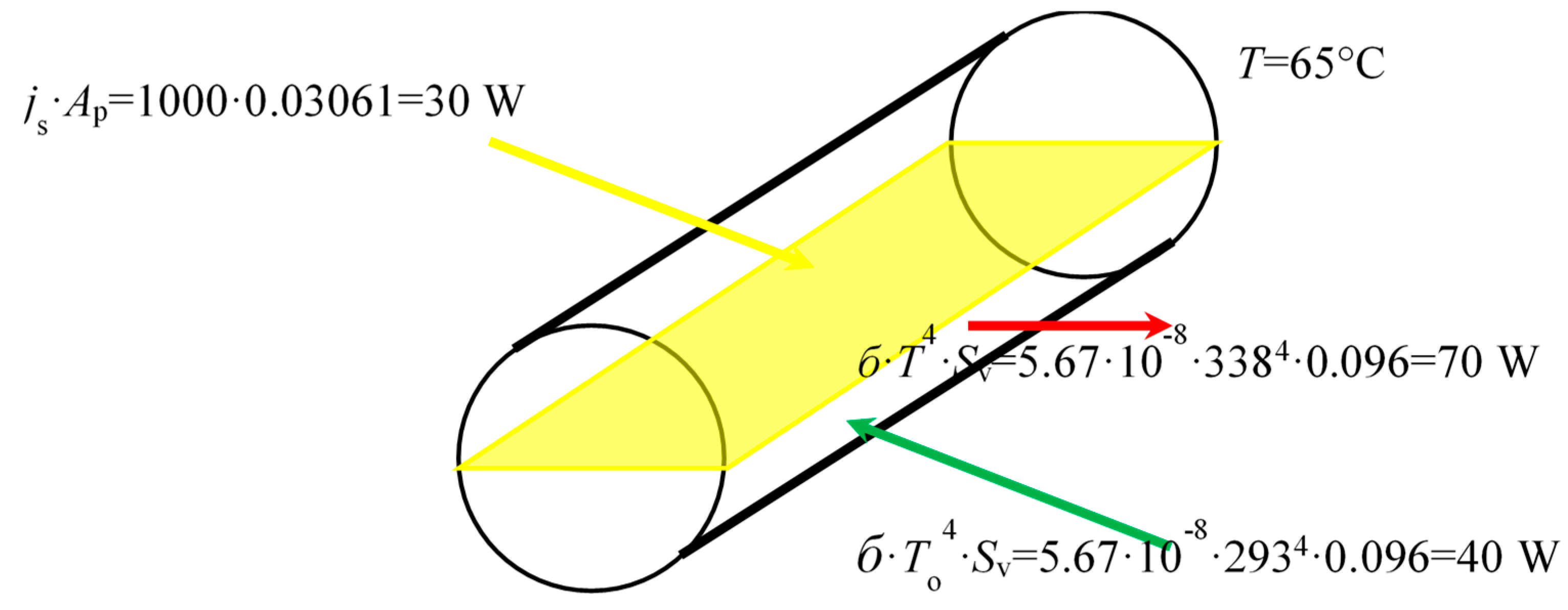
Figure 4.
Thermal balance of the cylinder in the sun, taking convection into account. Note: sun = 30 W, surrounding = 40 W, convection = 16 W, conductor at 43 °C = 54 W.
Figure 4.
Thermal balance of the cylinder in the sun, taking convection into account. Note: sun = 30 W, surrounding = 40 W, convection = 16 W, conductor at 43 °C = 54 W.
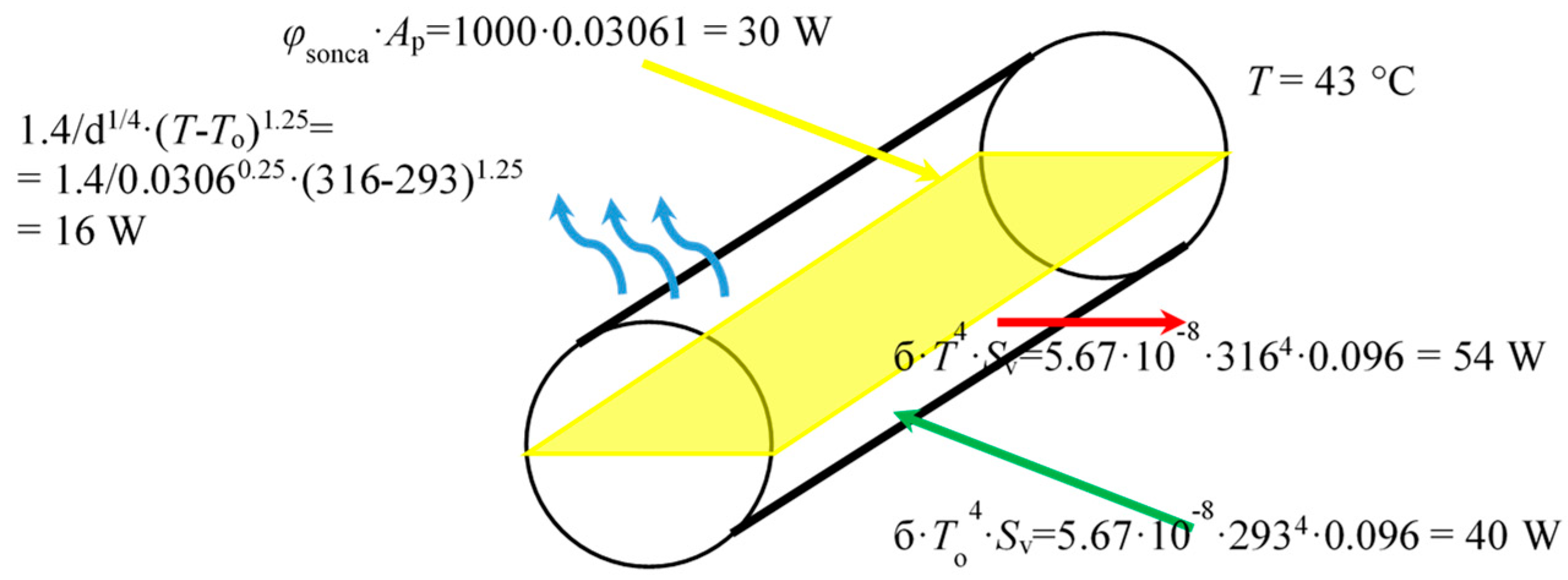
Figure 5.
The heat balance of the conductor in the sun, taking into account electrical heating and convection. Note: sun = 30 W, surrounding = 40 W, Joule’s heating = 70 W, convection = 55 W, conductor at 43 °C = 54 W.
Figure 5.
The heat balance of the conductor in the sun, taking into account electrical heating and convection. Note: sun = 30 W, surrounding = 40 W, Joule’s heating = 70 W, convection = 55 W, conductor at 43 °C = 54 W.
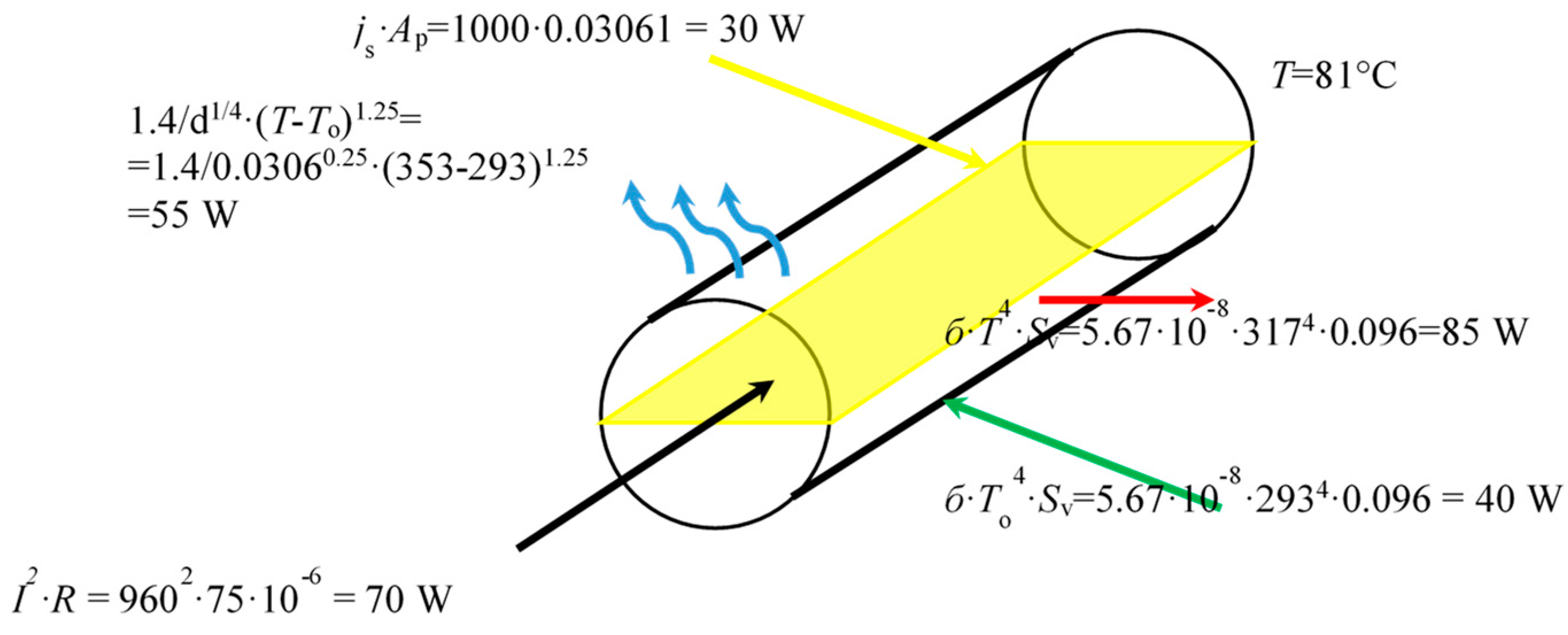
Figure 6.
Heat current from the steel core. Note: r is appropriate radius, T appropriate temperature, λ appropriate conductivity.
Figure 6.
Heat current from the steel core. Note: r is appropriate radius, T appropriate temperature, λ appropriate conductivity.
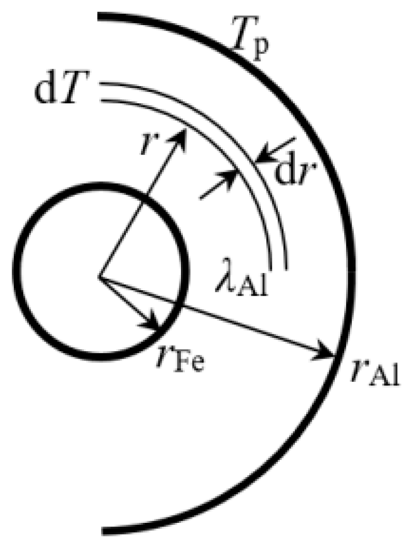
Figure 7.
Calculating the temperature in the steel core axis.

Figure 8.
(a) Measurement scheme with interrupted aluminum coat. (b) Picture of measurement with interrupted aluminum coat.
Figure 8.
(a) Measurement scheme with interrupted aluminum coat. (b) Picture of measurement with interrupted aluminum coat.
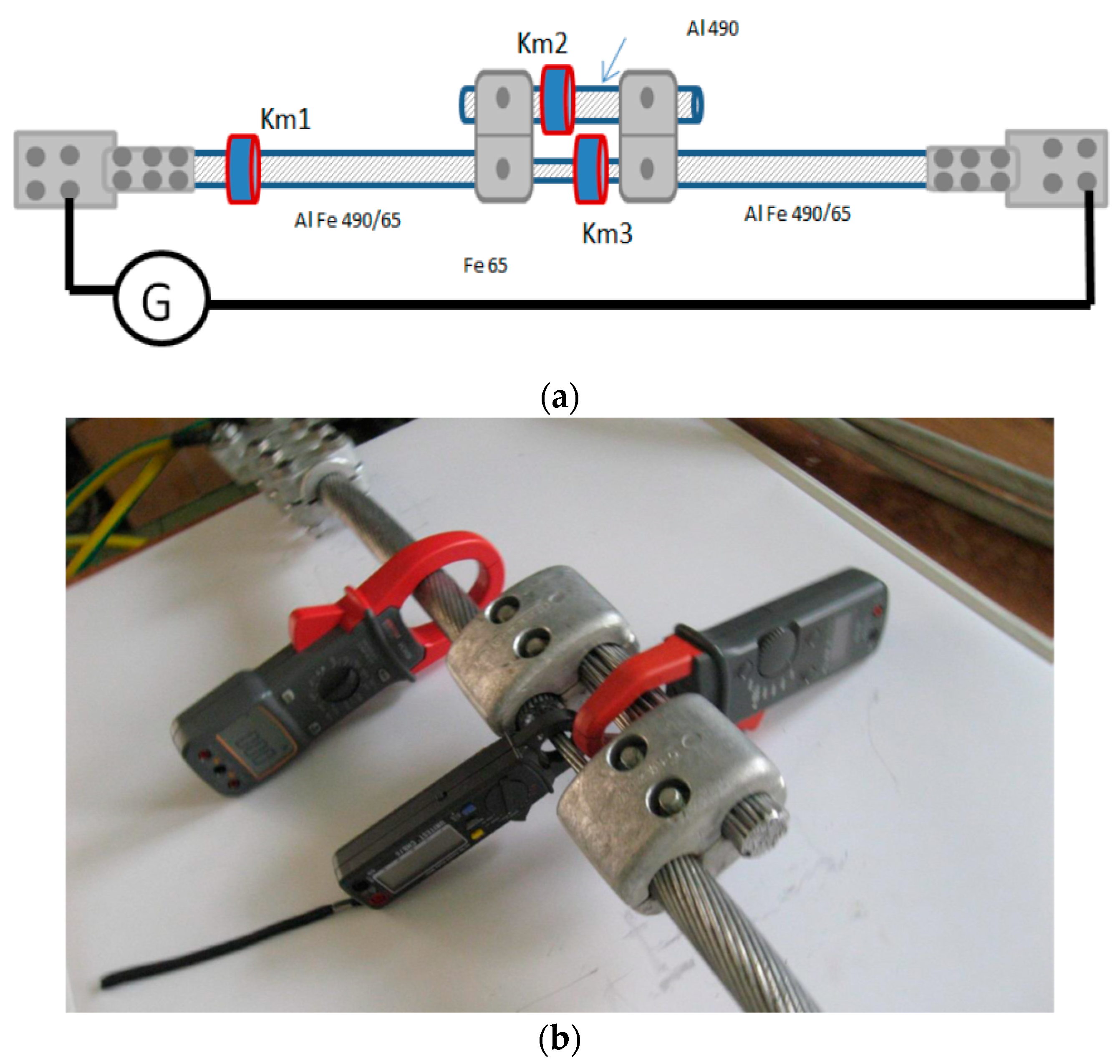
Figure 9.
Theoretical current distribution between the steel core and the aluminum coat. Picture of measurement with interrupted aluminum coat.
Figure 9.
Theoretical current distribution between the steel core and the aluminum coat. Picture of measurement with interrupted aluminum coat.
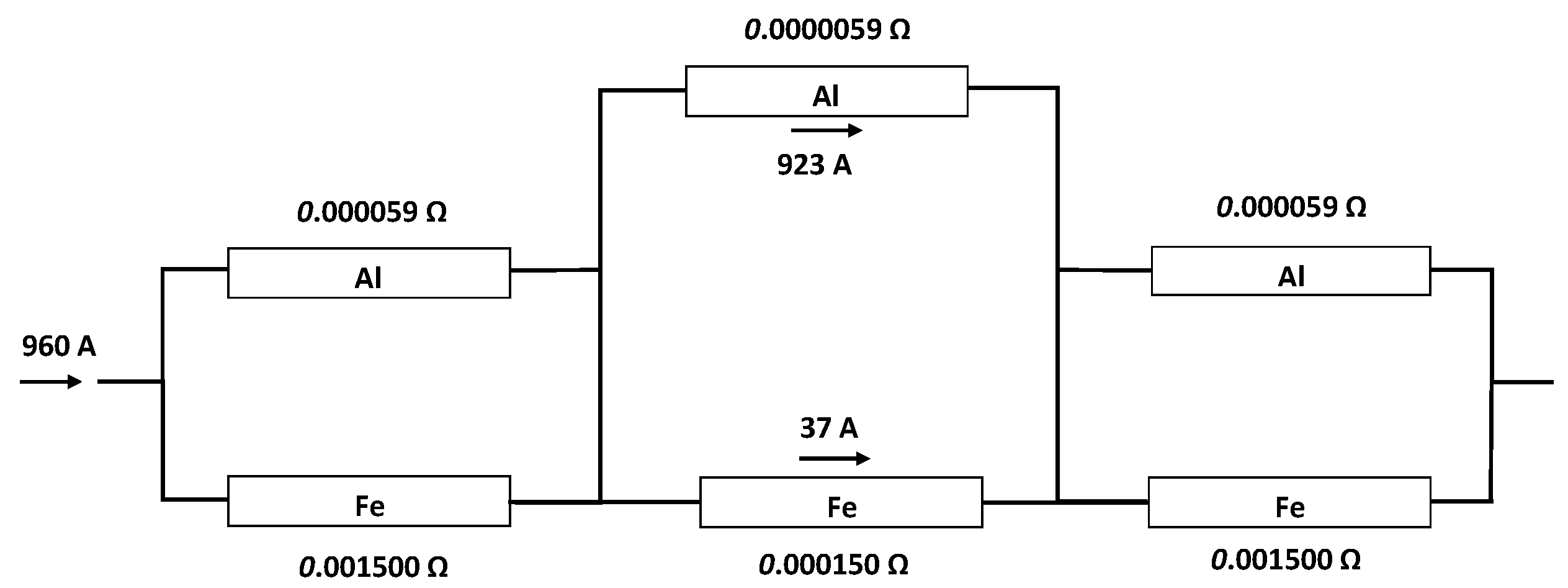
Figure 10.
Measurement of current in parallel binding of aluminum coat and steel core.
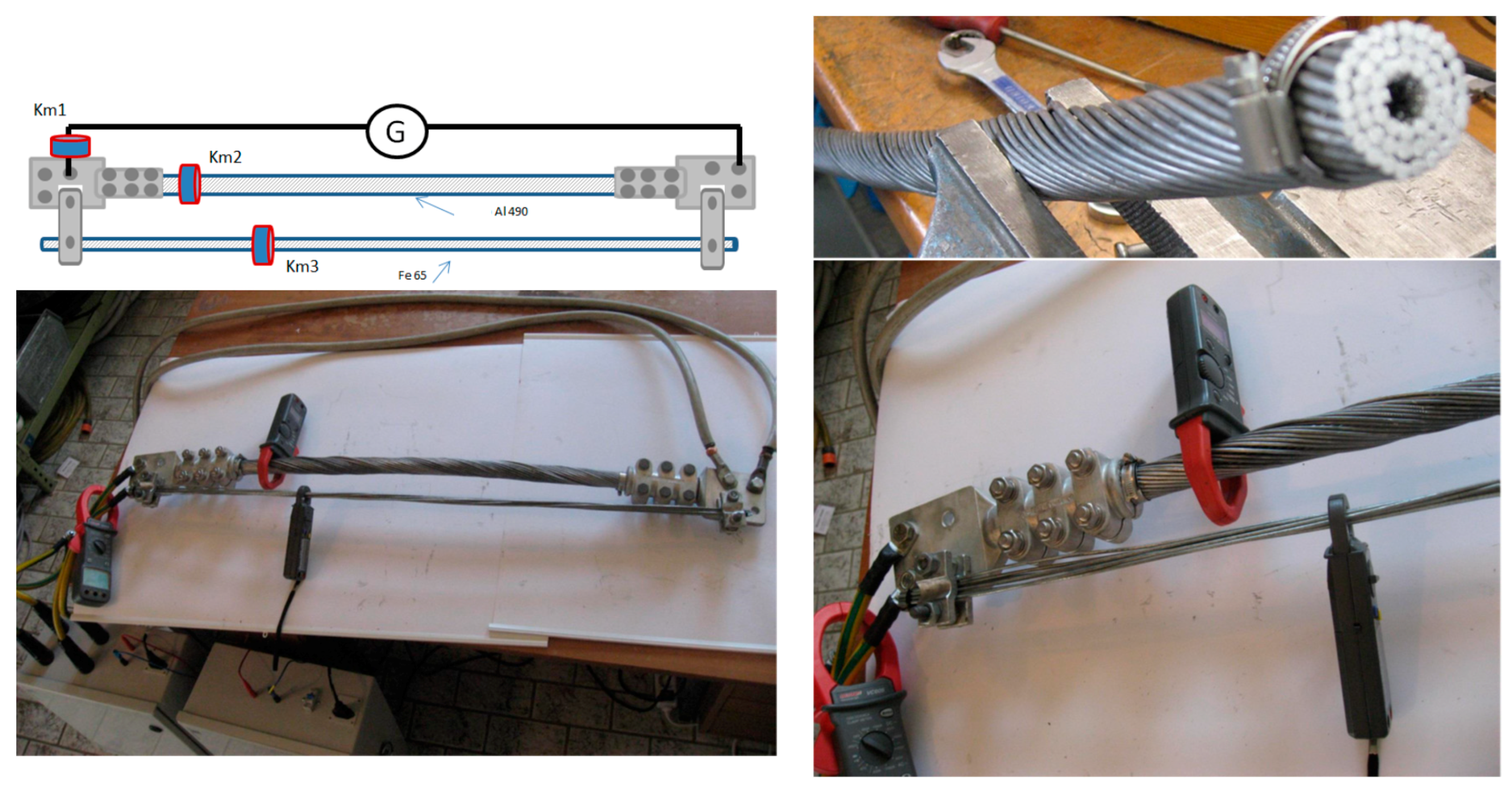
Figure 11.
Camera measured temperature at parallel binding.
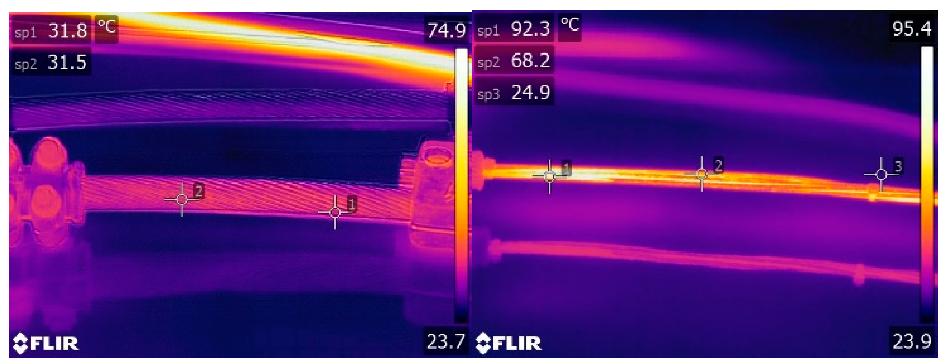
Figure 12.
Conductor with drawn replaced rings of air. Note: dark gray—circle and ring of metal (Fe) with the same surface as steel wires; light gray—the metal rings (Al) with the same surface as the wires in the individual layers; white—rings of air with the same surface as the empty spaces between the wires.

Figure 13.
Heat flow from the interior through the air layer.


Table 1.
Temperature in dependence of radius.
| Radius | r [m] | ϑ [°C] |
|---|---|---|
| rAl3 | 0.0153 | 50.80 |
| rAl2 | 0.0119 | 50.8088 |
| rAl1 | 0.0085 | 50.8148 |
| rFe2 | 0.0051 | 50.8177 |
| rFe1 | 0.0017 | 50.8212 |
| center | 0.0000 | 50.8223 |
I = 960 A, φ = 200 W/m2, To = 5 °C.
Table 2.
Results of measurement with interrupted aluminum coat.
| Current through the Clamp Meter Km1 [A] | Current through the Clamp Meter Km2 (Aluminum—Surface) | Current through the Clamp Meter Km3 (Steel—Core) | ||
|---|---|---|---|---|
| [A] | [ / ] | [A] | [ / ] | |
| 57 | 46 | 0.81 | 12 | 0.21 |
| 100 | 84 | 0.84 | 22 | 0.22 |
| 206 | 166 | 0.81 | 43 | 0.21 |
| 408 | 323 | 0.79 | 82 | 0.20 |
| 605 | 492 | 0.81 | 122 | 0.20 |
| 810 | 650 | 0.80 | 159 | 0.20 |
| 1004 | 811 | 0.81 | 198 | 0.20 |
| 1209 | 971 | 0.80 | 250 | 0.21 |
| 1406 | 1165 | 0.83 | 310 | 0.22 |
Table 3.
Measured and calculated currents and temperatures at parallel binding of steel core and aluminum coat.
Table 3.
Measured and calculated currents and temperatures at parallel binding of steel core and aluminum coat.
| Current through the Clamp Meter Km1 [A] | Clamp Meter Km2 (Aluminum—Surface) | Clamp Meter Km3 (Steel—Core ro) | ||||
|---|---|---|---|---|---|---|
| I [A] | T [°C] | I [A] | T [°C] | |||
| Measured * | Calculated | Measured * | Calculated | |||
| 57 | 56 | 25.7 | 25.9 | 2 | 25.3 | 25.9 |
| 104 | 99 | 26.3 | 4 | - | 26.3 | |
| 205 | 199 | 27.4 | 27.92 | 7 | - | 27.9 |
| 414 | 397 | 34.2 | 15 | - | 34.2 | |
| 611 | 593 | 41.7 | 43.6 | 22 | 47.9 | 43.6 |
| 814 | 792 | 56.4 | 29 | - | 56.4 | |
| 1005 | 986 | 71.4 | 37 | - | 71.4 | |
| 1210 | 1176 | 90.5 | 44 | - | 90.5 | |
| 1416 | 1370 | 92.3 | 112.8 | 50 | >160 | 112.9 |
* at higher current values, the stationary condition was not guaranteed.
Table 4.
Temperatures in dependency from radius and environmental conditions.
| Radius | r [m] | θ [°C] |
|---|---|---|
| rAl3 | 0.015 | 50.8 |
| rzrak4 | 0.012 | 50.807 |
| rAl2 | 0.011 | 52.319 |
| rzrak3 | 0.009 | 52.323 |
| rAl1 | 0.008 | 53.250 |
| rzrak2 | 0.006 | 53.253 |
| rFe2 | 0.005 | 53.479 |
| rzrak1 | 0.002 | 53.482 |
| rFe1 | 0.002 | 53.521 |
| center | 0.000 | 53.522 |
I = 960 A, φ = 200 W/m2, To = 5 °C.
Table 5.
Measured and calculated currents and temperatures at parallel binding of steel core and Aluminum coat taking into account the empty spaces.
Table 5.
Measured and calculated currents and temperatures at parallel binding of steel core and Aluminum coat taking into account the empty spaces.
| Current through the Clamp Meter Km1 | Clamp Meter Km2 (Aluminum—Surface) | Clamp Meter Km3 (Steel—Core ro) | ||||||
|---|---|---|---|---|---|---|---|---|
| Current | Temperature [°C] | Current | Temperature [°C] | |||||
| [A] | [A] | [ / ] | Measured | Calculated | [A] | [ / ] | Measured | Calculated |
| 57 | 56 | 98.25 | 25.7 | 25.9 | 2 | 3.51 | 25.3 | 26.1 |
| 104 | 99 | 95.19 | - | 26.3 | 4 | 3.85 | - | 26.1 |
| 205 | 199 | 97.07 | 27.4 | 27.9 | 7 | 3.41 | - | 27.9 |
| 414 | 397 | 95.89 | - | 34.3 | 15 | 3.62 | - | 37.1 |
| 611 | 593 | 97.05 | 41.7 | 43.9 | 22 | 3.60 | 47.9 | 50.9 |
| 814 | 792 | 97.30 | - | 57.3 | 29 | 3.56 | - | 73.9 |
| 1005 | 986 | 98.11 | - | 73.2 | 37 | 3.68 | - | 103.3 |
| 1210 | 1176 | 97.19 | - | 94.3 | 44 | 3.64 | - | 144.4 |
| 1416 | 1370 | 96.75 | 92.3 | 119.6 | 50 | 3.53 | >160 | 197.3 |
Note: at higher current values, the stationary condition was not guaranteed. We wanted to measure the steady state even also at the nominal current of the conductor, but we managed to complete the entire measurement only at 1370 A. During this current, the point source and the conductor were overloaded. The temperature meter (camera) showed more than 160 degrees. At this temperature, the measurement was interrupted, and 197 degrees were calculated.
© 2019 by the authors. Licensee MDPI, Basel, Switzerland. This article is an open access article distributed under the terms and conditions of the Creative Commons Attribution (CC BY) license (http://creativecommons.org/licenses/by/4.0/).
Share and Cite
MDPI and ACS Style
Voršič, Ž.; Maruša, R.; Pihler, J. New Method for Calculating the Heating of the Conductor. Energies 2019, 12, 2769. https://doi.org/10.3390/en12142769
AMA Style
Voršič Ž, Maruša R, Pihler J. New Method for Calculating the Heating of the Conductor. Energies. 2019; 12(14):2769. https://doi.org/10.3390/en12142769
Chicago/Turabian StyleVoršič, Žiga, Robert Maruša, and Jože Pihler. 2019. "New Method for Calculating the Heating of the Conductor" Energies 12, no. 14: 2769. https://doi.org/10.3390/en12142769
Note that from the first issue of 2016, this journal uses article numbers instead of page numbers. See further details here.