Accuracy Comparison of Coastal Wind Speeds between WRF Simulations Using Different Input Datasets in Japan

Abstract

In order to improve the accuracy of the wind speed simulated by a mesoscale model for the wind resource assessment in coastal areas, this study evaluated the effectiveness of using the Japan Meteorological Agency (JMA)’s latest and finest (2 km × 2 km) grid point value (GPV) data, produced from the local forecast model (LFM) as input data to the mesoscale model. The evaluation was performed using wind lidar measurements at two sites located on the coasts of the Sea of Japan and Pacific Ocean. The accuracy of the LFM–GPV was first compared with that of two products from the JMA Meso Scale Model (MSM) (5 km × 5 km): MSM-GPV and mesoscale analysis (MANAL). Consequently, it was shown that LFM–GPV exhibited the most accurate wind speeds against lidar measurements. Next, dynamical downscaling simulations were performed using the weather research and forecasting model (WRF) forced by the three datasets above, and their results were compared. As compared to the GPVs, it was found that the WRF dynamical downscaling simulation using them as input can improve the accuracy of the coastal wind speeds. This was attributed to the advantage of the WRF simulation to improve the negative bias from the input data, especially for the winds blowing from the sea sectors. It was also found that even if the LFM–GPV is used as an input to the WRF simulation, it does not always reproduce more accurate wind speeds, as compared to the simulations using the other two datasets. This result is partly owing to the tendency of WRF to overestimate the wind speed over land, thus obscuring the higher accuracy of the LFM–GPV. It was also shown that the overestimation tendency cannot be improved by only changing the nudging methods or the planetary boundary layer schemes in WRF. These results indicate that it may be difficult to utilize the LFM–GPV in the WRF wind simulation, unless the overestimation tendency of WRF itself is improved first.

1. Introduction

In March 2017, the New Energy and Industrial Technology Development Organization (NEDO) released the Japanese offshore wind resource map, NEDO Offshore Wind Information System (NeoWins) [1]. It provides the annual mean wind speed distributions and detailed wind climate statistics at five heights from 60 to 140 m, with a spatial resolution of 0.5 km × 0.5 km for coastal waters within 30 km from the coast, and with a spatial resolution of 0.100° × 0.125° for open oceans within the Japanese Economic Exclusive Zone. In addition, NeoWins offers wind information and any information regarding natural and social environmental conditions required for offshore wind energy development. Thus, NeoWins has become a powerful tool for planning offshore wind farms in Japan.

The wind information of NeoWins was produced using the weather research and forecasting model (WRF) [2], which is a mesoscale meteorological model frequently used for offshore wind resource assessment (e.g., [3,4,5,6,7,8]). The accuracy of wind speeds with a spatial resolution of 0.5 km × 0.5 km was examined using wind turbine hub-height measurements from three meteorological masts and a wind lidar at four coastal sites [9,10,11]. Subsequently, it was confirmed that the target accuracy of the map (the relative bias is within ±5% for the annual mean wind speed at a hub height) was achieved at all the sites. This result means that though the resolution of 0.5 km × 0.5 km is in the so-called “gray zone” [12], and the WRF simulation exhibits accurate wind speeds. However, considering the spread of the offshore wind development in the near future, it is important to obtain more accurate wind speed simulated by WRF, as WRF is used for dynamical downscaling for a specific site and will used for the next-generation wind resource map.

The choice of input data is crucial for a dynamical downscaling. Thus, the sensitivity of the input data to the mesoscale model simulation has often been discussed in previous studies (e.g., [13,14,15,16,17]). In NeoWins, mesoscale analysis (MANAL) [18], which is the objective analysis with a spatial resolution of 5 km × 5 km produced by the Japan Meteorological Agency (JMA), is used as initial and lateral boundary conditions to force WRF. Akimoto and Kusaka (2010) [19] showed that the use of MANAL for the downscaling provides more accurate weather conditions in the Kanto Plain, Japan, than that of the National Centers for Environmental Prediction (NCEP)-final operational global analysis (FNL) with a spatial resolution of 1° × 1° [20]. In addition to MANAL, two other grid point values (GPVs) can be utilized as input data to WRF: Local forecast model (LFM)–GPV [21] and meso scale model (MSM)–GPV [22], which are numerical weather prediction data from the JMA LFM and MSM, respectively. The LFM is the latest and finest nonhydrostatic model introduced in August 2012, and is designed to allow for the rapid production and frequent updating of analyses at a higher resolution (2 km × 2 km, hourly). Our previous study [23] evaluated the accuracy of wind speeds derived from the LFM–GPV and the MSM–GPV using in-situ onshore and offshore measurements obtained at the low altitudes less than 40 m above ground level (AGL). They indicated that the wind speeds of the LFM–GPV were more accurate than those of the MSM–GPV for both onshore and offshore, and presumed that the result was attributed to higher temporal and spatial resolutions and the assimilation of data from the automated meteorological data acquisition system (AMeDAS), operated by the JMA. Therefore, we expect that the accuracy of wind speed in the WRF simulation can be improved partially using the LFM–GPV as input data.

This study aimed to examine whether using the LFM–GPV would result in a more accurate WRF simulation for wind resource assessment in coastal areas, as compared to the cases using the MSM–GPV and MANAL. The wind speeds of the LFM–GPV, MSM–GPV, and MANAL, and the WRF simulations forced by them were compared with wind lidar measurements at two coastal sites in Japan. In-situ observations, input data, model configurations, and evaluation methods are described in Section 2. The accuracies of the GPV and WRF wind speeds are compared and evaluated in Section 3. Section 4 discusses the possible methods to improve the accuracy of the WRF simulation, and the conclusions of this study are presented in Section 5.

2. Observation Data and Evaluation Method

2.1. In-Situ Observation Data

Figure 1 shows the maps of Japan and target areas, i.e., Niigata and Ibaraki, which are located on the coasts of the Sea of Japan and the Pacific Ocean, respectively. They exhibit different wind climatology and are thus suitable for the evaluation of the WRF simulation in the coasts of Japan.

Table 1. Specifications of lidar observations at Niigata and Ibaraki.

Site	Niigata	Ibaraki
Manufacturer	ZephIR Lidar	Leosphere
Measurement	ZephIR 300	WindCube WLS7-86
Vertical Level	40, 58, 80, 95, 145 m	47, 67, 87, 107, 127, 147, 167, 187, 207 m

shows the specifications of lidar observations at both sites. At Niigata, lidar measurements were performed on flat land at approximately 300 m inland from the coastline. The ZephIR 300 lidar [24] was used to measure the wind speed and direction at the heights of 40, 58, 80, 95, and 145 m above mean sea level (AMSL). At Hazaki, the WindCube WLS7-86 lidar [25] was installed at the tip of a 427-m long pier owned by the Hazaki Oceanographic Research Station [26] of the Port and Airport Research Institute (PARI). Vertical wind profiles from 47 to 207 m AMSL were measured with an interval of 20 m. The lidar measurements are accurately calibrated by using the different in-situ measurements: The meteorological mast at Niigata (Mito et al., 2016 [27]), and another lidar measurement at Ibaraki (Shimada et al., 2018 [28]). The heights of 95 m at Niigata and 107 m at Ibaraki are referred to as a “hub height” in this study. The lidar data of the 10-min average wind speed and direction at every height for a whole year (from October 2015 to September 2016) was used for the analyses.

Figure 2 shows the annual wind roses at Niigata (95 m) and Ibaraki (107 m). The prevailing wind directions are northwest and east for Niigata, and north–northeast and south–southwest for Ibaraki. The NW winds at Niigata have a higher speed than the E winds, while the NNE and SSW wind speeds at Ibaraki are similar. To investigate the accuracy of wind speeds from GPVs and WRF simulations, which is considered to depend on wind direction, it is convenient to define the land and sea sectors for wind direction. Considering the shape of the coastlines at Niigata and Ibaraki, the sectors are defined as indicated by the red dot lines in Figure 1b,c. At Niigata, the land and sea sectors are 0° ≤ θ < 225° and 225° ≤ θ < 360°. At Ibaraki, the land sector is 150° ≤ θ < 330° and the sea sector is 0° ≤ θ < 150° or 330° ≤ θ < 360°. When the wind directions at all of the measurement heights are classified into one of each sector, the wind is defined as that for the sector.

Table 2. Number of samples of wind speed data for the land sector (land), sea sector (sea), and others (other), and the total for the year (annual).

Sector	Niigata	Ibaraki
land	3937 (55%)	2276 (32%)
sea	2603 (37%)	4177 (59%)
other	580 (8%)	615 (9%)
annual	7120 (100%)	7068 (100%)

shows the number of samples of wind speed data for each sector. Niigata has more winds from the land sector (ENE to E), while Ibaraki has more winds from the sea sector (NNE to NE). “Other” in the table implies cases where the sector cannot be identified owing to non-uniform wind directions with height.

2.2. JMA GPVs

The LFM and MSM are the current forecasting models for disaster prevention and aviation safety, operated by the JMA. The horizontal resolution for the surface and pressure layer is 2 km × 2 km (1531 × 1301 grids) in the LFM and 5 km × 5 km (817 × 661 grids) in the MSM. The number of vertical levels in the LFM is 58 from the surface to 20.2 km and that of the MSM is 48 from the surface to 21.8 km. The LFM uses forecasting results from the MSM as the lateral boundary condition, and is designed to provide shorter-range forecasting with a higher spatio–temporal resolution. In the forecast cycle, the first guesses from the LFM and MSM are combined with the latest multiple observations through data assimilation, producing the local analysis (LANAL) and MANAL, respectively. It is noteworthy that only LANAL assimilates surface data from AMeDAS to improve the reproducibility of local-scale phenomena. More details on the models and data assimilation systems are available in the JMA report [29].

The GPVs from the LFM and MSM, including LANAL and MANAL, are distributed by the Japan Meteorological Business Support Center (JMBSC). Because LANAL is a new dataset and available only after January 2018, this study used three GPVs from the LFM (hereinafter called LFM–GPV), MSM (hereinafter called MSM–GPV), and MANAL, which are available for the study period from October 2015 to September 2016.

Table 3. Specifications of the LFM–GPV, MSM–GPV, and MANAL [18,21,22].

GPV		LFM–GPV	MSM–GPV	MANAL
Horizontal Resolution	Surface Level	0.025° × 0.020° (1201 × 1261 grids)	0.0625° × 0.0500° (481 × 505 grids)	5 km × 5 km (721 × 577 grids)
	Pressure Level	0.050° × 0.040° (601 × 631 grids)	0.1250° × 0.1000° (241 × 253 grids)	5 km × 5 km (721 × 577 grids)
Vertical Layers		17 levels	17 levels	16 levels
Temporal Resolution		1 hourly (00, 01, ..., 23 UTC)	3 hourly (00, 03, ..., 21 UTC)	3 hourly (00, 03, ..., 21 UTC)
Forecast Range		9 h	39 h	none

shows the specifications of those three GPVs. The GPVs include the islands of Japan and their surrounding waters, having horizontal resolutions of 0.025° × 0.020° (LFM–GPV), 0.0625° × 0.0500° (MSM–GPV), and 5 km × 5 km (MANAL) for the surface layer. The number of vertical layers of the LFM–GPV and MSM–GPV are both 17, and includes the surface layer and 16 pressure levels (1000, 975, 950, 925, 900, 850, 800, 700, 600, 500, 400, 300 250, 200, 150, and 100 hPa). MANAL has the same levels except for 975 hPa. The primary parameters included in the datasets are sea-level pressure, geopotential height, wind speed, temperature, relative humidity, etc. As for the LFM–GPV and MSM–GPV, only the initial values of each forecasting cycle (not forecast values) were used in this study.

To extract the wind speed at an arbitrary point from the GPVs, bilinear interpolation was used for the horizontal plane. For height, a linear–log interpolation was applied in the U-logZ plane, using three wind speeds at 10 m AGL and at the AGL heights of the two lowest pressure levels, following our previous study [23].

2.3. WRF Configuration

In this study, the Advanced Research WRF (ARW) version 3.8.1 [2] was used as a meteorological mesoscale model. The 12 one-month WRF simulations were performed for whole a year from October 2015 to September 2016. Figure 1b,c show the model domains for Niigata and Ibaraki, and

Table 4. Model configuration used for WRF simulations.

Method		Advanced Research WRF (ARW) Version 3.8.1
Period		1 year (from October 2015 to September 2016)
Input Data		Soil: NCEP-FNL (6 hourly, 1° × 1°) SST: AIST-Kobe Univ. MOSST (daily, 0.02° × 0.02°)
Terrain Data	Domain 1	Elevation: USGS GTOPO30 Land use: USGS 24 land-use categories data (30″ × 30″)
	Domain 2	Elevation: METI-NASA ASTER GDEM (1″ × 1″) Land use: MLIT NLNI (0.1 km × 0.1 km)
Vertical Levels		40 levels (Surface to 100 hPa) Lowest half levels: 23 m, 73 m, 130 m, 199 m, 287 m, ...
FDDA	Domain 1	Enabled (u, v, θ, q)
	Domain 2	Enabled (u, v, θ, q), excluding interior of PBL
Physics Options		Shortwave process: Dudhia scheme Longwave process: Rapid Radiative Transfer Model scheme Cloud microphysics process: Ferrier (new Eta) scheme PBL Process: MYJ (Eta operational) scheme Surface layer process: Monin–Obukhov (Janjic Eta) scheme Land-surface process: Noah land surface model scheme Cumulus parameterization: None

shows the model configuration used for the simulations. The model configuration follows that used for the NeoWins project [1]. The roughness length used in the WRF simulation is based in the land-use data from the National Land Numerical Information (NLNI), which has 12 categories in land-use [30]. The value of roughness length was set so that it was similar to the original value for the United States Geological Survey (USGS) land-use category [31]. The soil temperature and moisture used for the Noah land surface model [32] were obtained from NCEP-FNL (1° × 1°, 6 hourly). The sea surface temperature (SST) based on a moderate resolution imaging spectroradiometer (MODIS) (0.02° × 0.02°, daily) (MOSST), developed by the National Institute of Advanced Industrial Science and Technology (AIST) and Kobe University [33], was used as the lower boundary condition. The number of vertical levels was 40 from the surface to 100 hPa, and the lowest levels were located at approximately 23, 73, 130, 199, and 287 m AGL. Four-dimensional data assimilation (FDDA) was conducted by applying the grid nudging to full levels in the outer domain, and to the levels above the top of the planetary boundary layer (PBL) in the inner domain, where the horizontal components of the wind speed (u, v), potential temperature (θ), and water vapor mixing ratio (q) are nudged toward the GPVs. As a PBL scheme, the Mellor–Yamada–Janjic (MYJ) scheme [34] was used because it has often been adopted in previous studies (e.g., [1,35,36,37]).

Table 5. Input data and model grids used in WRF–LFM, WRF–MSM, and WRF–MANAL simulations.

Case		WRF–LFM	WRF–MSM	WRF–MANAL
Input Data		LFM–GPV (3 hourly)	MSM–GPV (3 hourly)	MANAL (3 hourly)
Grids	Domain 1	1.5 km × 1.5 km (168 × 168 grids)	2.5 km × 2.5 km (100 × 100 grids)	2.5 km × 2.5 km (100 × 100 grids)
	Domain 2	0.5 km × 0.5 km (201 × 201 grids)	0.5 km × 0.5 km (200 × 200 grids)	0.5 km × 0.5 km (200 × 200 grids)

shows the input data and model grids used in the three WRF simulations. Considering the horizontal resolutions of the LFM–GPV (0.025° × 0.020°), MSM–GPV (0.0625° × 0.0500°), and MANAL (5 km × 5 km), the WRF simulation using the LFM–GPV as input (hereinafter called WRF–LFM) contains 1.5 to 0.5 km domains, while those using MSM–GPV and MANAL (WRF–MSM and WRF–MANAL, respectively) contains 2.5 to 0.5 km domains. In order to capture large-scale meteorological conditions from the GPVs, the outer domains were set to the rectangular area with the side of about 250 km. This study used the 3 hourly initial values of the GPVs as lateral boundary conditions to force WRF, and for data assimilation. For accuracy evaluation, hourly WRF wind speeds at observation points, expected from the inner domain using bilinear and linear-log interpolations, were compared with in-situ measurements.

2.4. Evaluation Methods

The accuracies of the GPV and WRF wind speeds were evaluated using three statistical parameters: Bias, root mean square error (RMSE), and correlation coefficient. They are written as follows:

$$\mathrm{bias}=\frac{1}{n}{\displaystyle \sum _{i=1}^n\left(W_{\mathrm{EST},i}-W_{\mathrm{OBS},i}\right)},$$

(1)

$$\mathrm{RMSE}=\sqrt{\frac{1}{n}{\displaystyle \sum _{i=1}^n{\left(W_{\mathrm{EST},i}-W_{\mathrm{OBS},i}\right)}^2}},$$

(2)

$$r=\frac{\frac{1}{n}{\displaystyle \sum _{i=1}^n\left(W_{\mathrm{EST},i}-{\overline{W}}_{\mathrm{EST}}\right)\left(W_{\mathrm{OBS},i}-{\overline{W}}_{\mathrm{OBS}}\right)}}{\sqrt{\frac{1}{n}{\displaystyle \sum _{i=1}^n{\left(W_{\mathrm{EST},i}-{\overline{W}}_{\mathrm{EST}}\right)}^2}}\sqrt{\frac{1}{n}{\displaystyle \sum _{i=1}^n{\left(W_{\mathrm{OBS},i}-{\overline{W}}_{\mathrm{OBS}}\right)}^2}}},$$

(3)

where n is the number of data samples, $W_{\mathrm{EST},i}$ is the GPV or WRF wind speed, $W_{\mathrm{OBS},i}$ is the observed wind speed, and ${\overline{W}}_{\mathrm{EST}}$ and ${\overline{W}}_{\mathrm{OBS}}$ are temporal averages for each wind speed. In this study, the bias and RMSE are presented using relative values (%), i.e., those normalized by the observed mean wind speed, because a relative value is customarily used in the research of wind energy and its application.

3. Accuracy Comparison of Wind Speeds

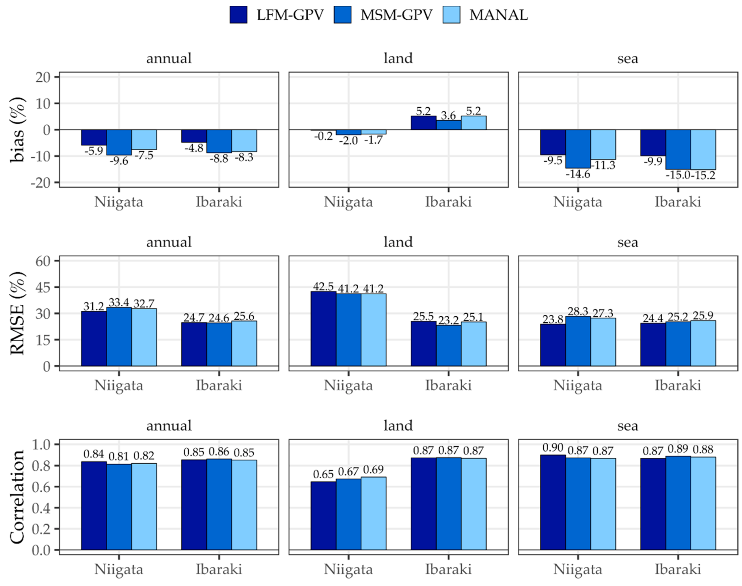
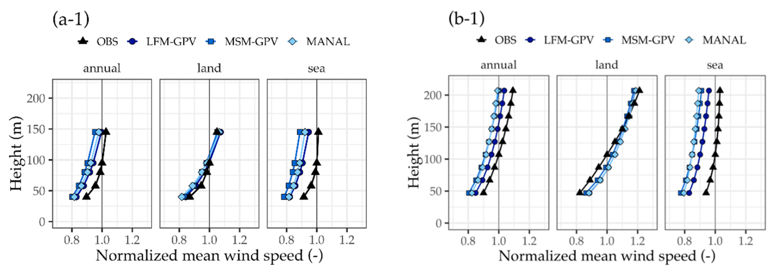
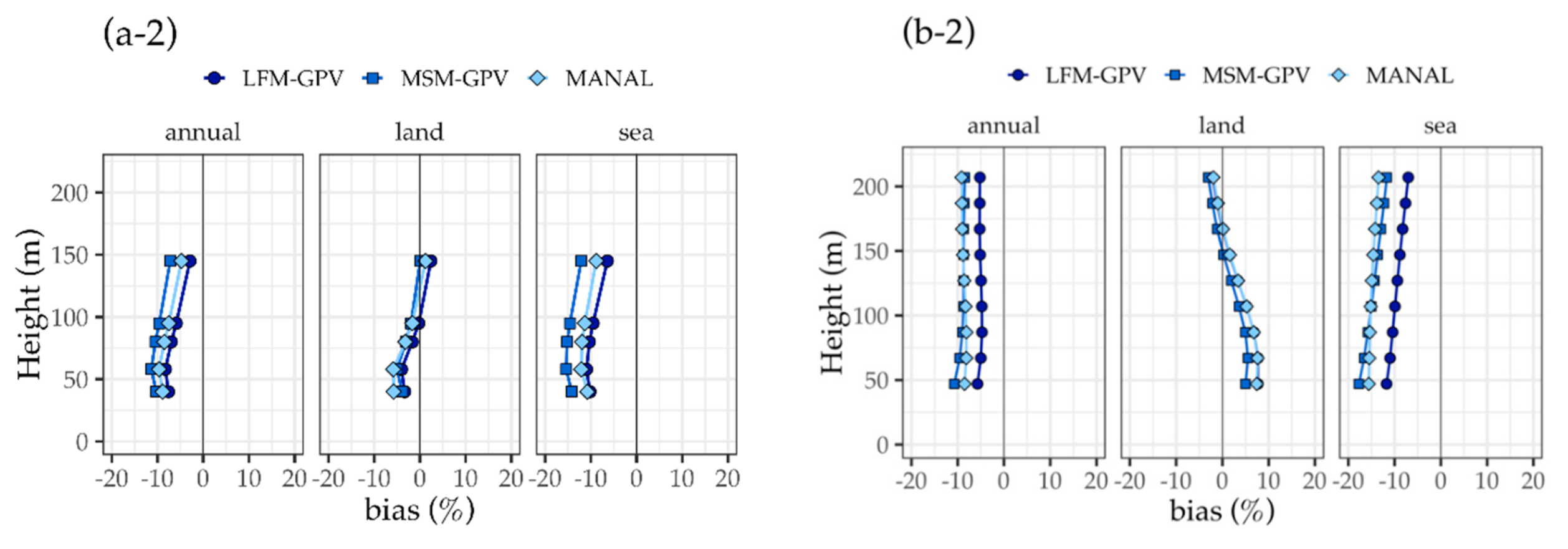
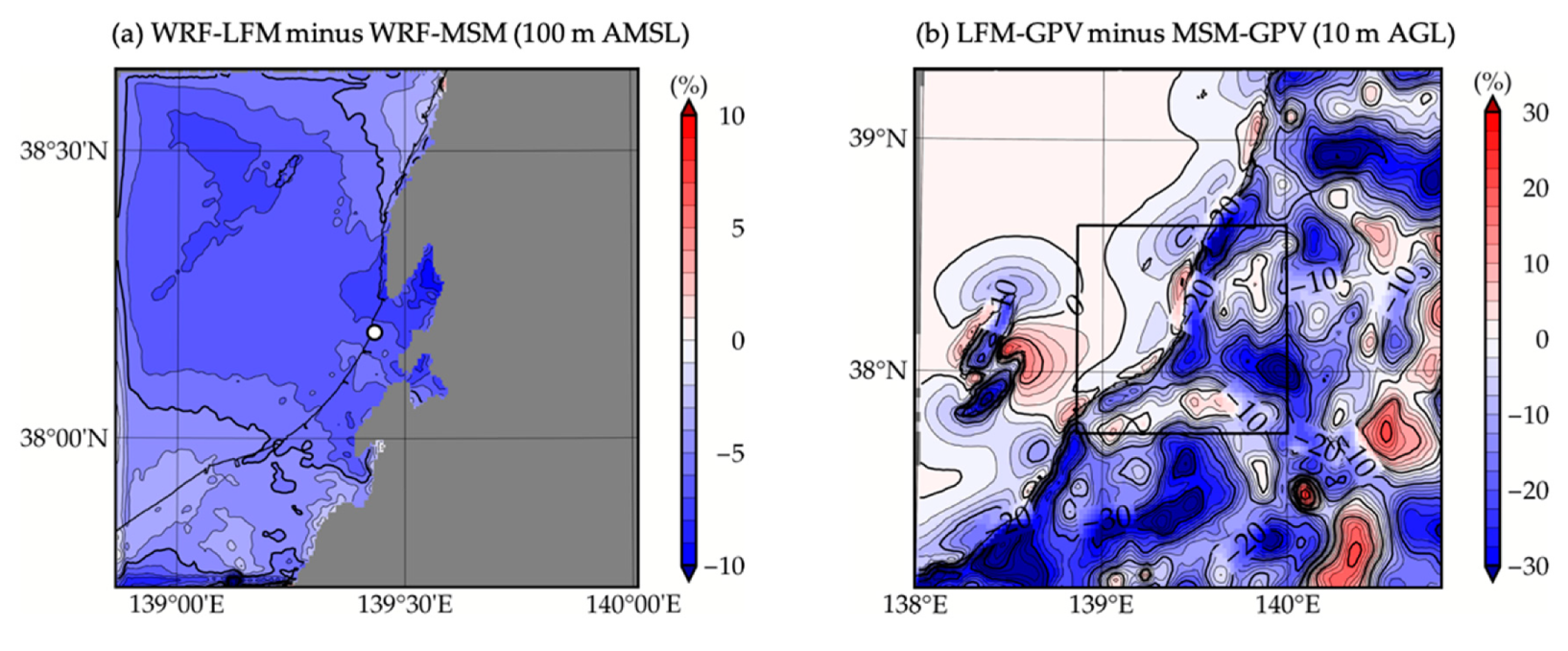
3.1. Comparison between GPV Wind Speeds

First, we investigated the accuracy of wind speeds from the three GPVs. Note that the annual mean wind speed at Ibaraki (107 m) is 7.85 m/s, though that at Niigata cannot be specified in this study due to the agreement with the data providers. Figure 3 shows the annual biases, RMSEs, and correlation coefficients of the GPV wind speeds at Niigata (95 m) and Ibaraki (107 m). The annual biases of the LFM–GPV, MSM–GPV, and MANAL were −5.9%, −9.6%, and −7.5% at Niigata, respectively, and −4.8%, −8.8%, and −8.3% at Ibaraki, respectively. The biases were all negative, meaning that the GPVs underestimate the annual mean wind speed at both sites. Dividing the winds into those coming from the land and sea sectors, the biases of the LFM–GPV, MSM–GPV, and MANAL for the land-sector winds were −0.2%, −2.0%, and −1.7% at Niigata, respectively, and 5.2%, 3.6%, and 5.2% at Ibaraki, respectively, whereas those for the sea-sector winds were −9.5%, −14.6%, and −11.3% at Niigata, respectively, and −9.9%, −15.0%, and −15.2% at Ibaraki, respectively. All of the GPVs remarkably underestimated the wind speed for the sea-sector winds at both sites, whereas the biases of the land-sector winds were closer to zero. These results indicate that the negative biases of the annual mean wind speeds are primarily caused by the sea-sector winds. The results of the GPVs underestimating the sea-sector winds (winds having been blowing on the sea surface) and overestimating the land-sector winds (winds having been blowing on the land surface) are in good agreement with those shown in our previous study [23], although the study examined the surface winds. The only exception is the underestimation for the land-sector wind at Niigata. For this wind, the GPVs exhibited RMSEs of 41.2% to 42.5% and correlation coefficients of 0.65 to 0.69, i.e., a much lower accuracy than those of other winds. The low accuracy is attributed to the low wind speed of the predominant ENE–E winds (as shown in Figure 2a), which are primarily land breezes at night (shown later). It is speculated that the MSM–GPV and MANAL cannot reproduce such local winds well, owing to its low spatial resolutions.

Figure 4 shows the vertical profiles of the GPV and the observed mean wind speeds and its difference (bias) at Niigata and Ibaraki. Here, the wind speeds were normalized by the observed mean wind speed at the hub height (95 m at Niigata and 107 m at Ibaraki). The biases were normalized by the observed mean wind speed at each height. From this figure, it is found that the three GPVs exhibited negative annual biases; that is, the GPVs underestimate the annual mean wind speeds at both the hub heights and other heights. In the bias profiles for the land-sector and sea-sector winds, the absolute values were found to increase toward the surface, including positive biases found for the land-sector winds at Ibaraki. This finding is consistent with the result of Shimada et al. (2011b) [36] that indicated a similar tendency of MANAL wind speeds using wind profiler measurements at 10 JMA stations.

Next, the accuracies of the three GPV wind speeds were compared. Figure 3 and Figure 4 show that the LFM–GPV tends to exhibit higher wind speeds than the other GPVs, and hence exhibited the smallest (reduced negative) biases. The annual RMSEs of the LFM–GPV, MSM–GPV, and MANAL were 31.2%, 33.4%, and 32.7% at Niigata, respectively, and 24.7%, 24.6%, and 25.6% at Ibaraki, respectively; meanwhile, the annual correlation coefficients were 0.84, 0.81, and 0.82 at Niigata, respectively, and 0.85, 0.86, and 0.85 at Ibaraki, respectively. It is found that the two statistical parameters were not significantly different between the three GPVs, and the same holds for each of the land-sector and sea-sector winds. Therefore, the accuracy comparison between the GPVs results in the conclusion that the LFM–GPV provides the most accurate wind speeds at all the heights of both sites. The high accuracy of the LFM–GPV is likely owing to its higher spatio–temporal resolution and the data assimilation of AMeDAS data, as discussed in our previous study [23].

3.2. Comparison between GPV and WRF Wind Speeds

This subsection compares the wind speeds simulated by WRF using the three GPVs discussed in the previous subsection, as the input. Figure 5 shows the annual biases, RMSEs, and correlation coefficients for the three WRF wind speeds: WRF–LFM, WRF–MSM, and WRF–MANAL. The annual biases for the WRF–LFM, WRF–MSM, and WRF–MANAL were −2.8%, −0.1%, and 1.5% at Niigata, respectively, and 3.7%, 1.2%, and 2.7% at Ibaraki, respectively. Compared to the biases of GPVs (Figure 3), the absolute values of the biases, especially those for the sea-sector wind, were significantly smaller at both sites. When comparing Figure 4 (showing the GPV wind profiles) and Figure 6 (showing the WRF wind profiles), improvements are shown for all the observation heights. This appears to be the effect of the higher spatio–temporal downscaling with WRF.

Figure 6 also shows that the biases for the land-sector wind were negative at Niigata and positive at Ibaraki for all the heights, and the bias tendency increased toward the surface. However, the former result in that the bias was negative is inconsistent with the results of previous studies [11,35,36,37] that reported the tendency of a positive bias over land for the WRF wind speeds. To explain this discrepancy, Figure 7 shows the accuracy variations of the WRF wind speed in a day at Niigata. As shown, a negative bias appeared from 22 to 8 LST, primarily at night. Because the number of samples was significantly larger at night (Figure 7a) and the wind speed from the land sector was low (Figure 2a), the wind at night is primarily considered as a typical land breeze, blowing from the ENE or E. The result above indicates that WRF tends to underestimate the land breeze circulating at night. Meanwhile, during the day, positive biases prevail that are likely the same type of positive bias as those reported in the previous studies [11,35,36,37]. In other words, the negative bias found at Niigata is caused by another tendency of WRF, which generally tends to overestimate the wind speed over land.

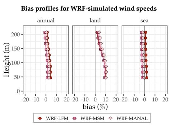
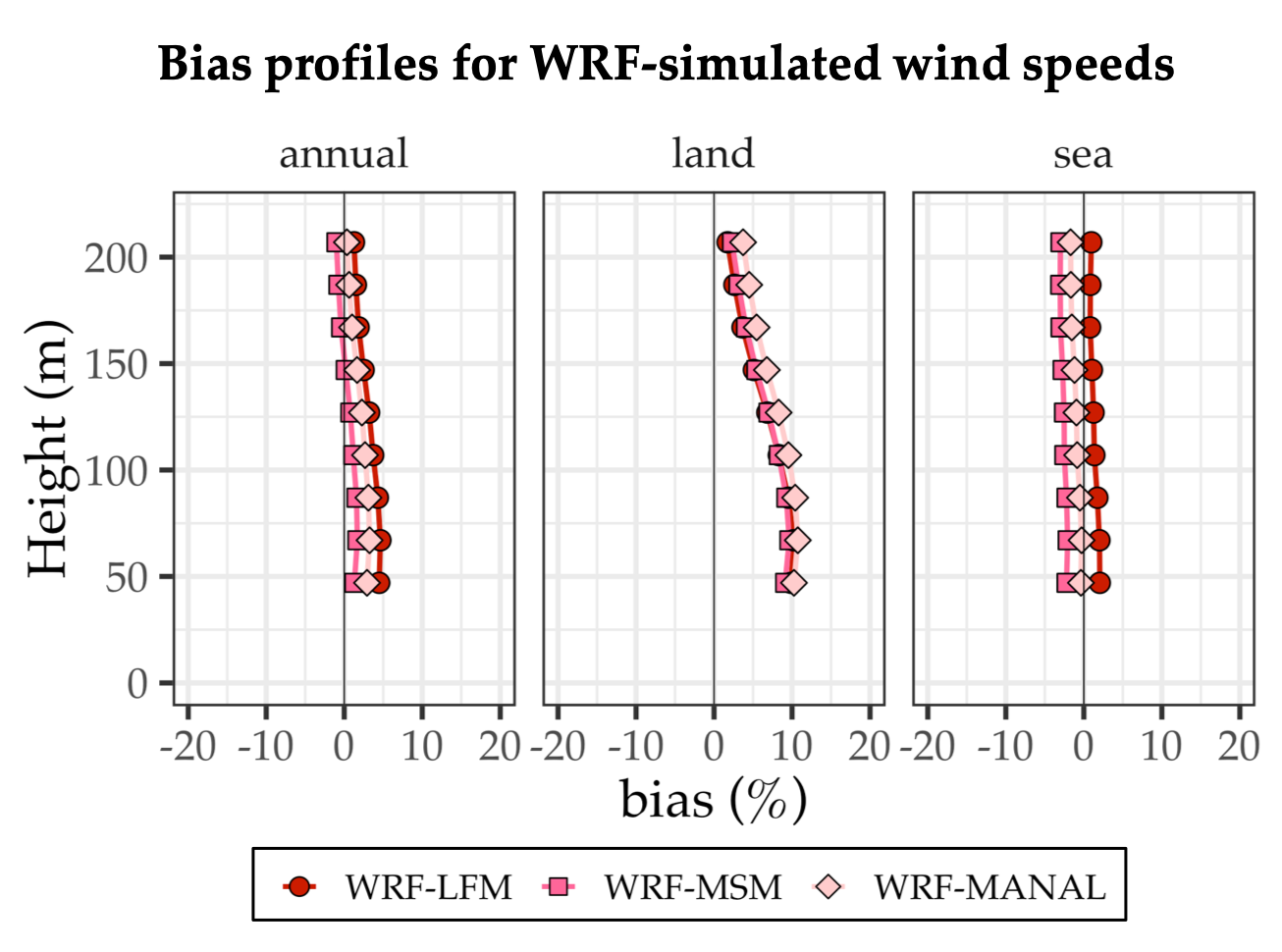
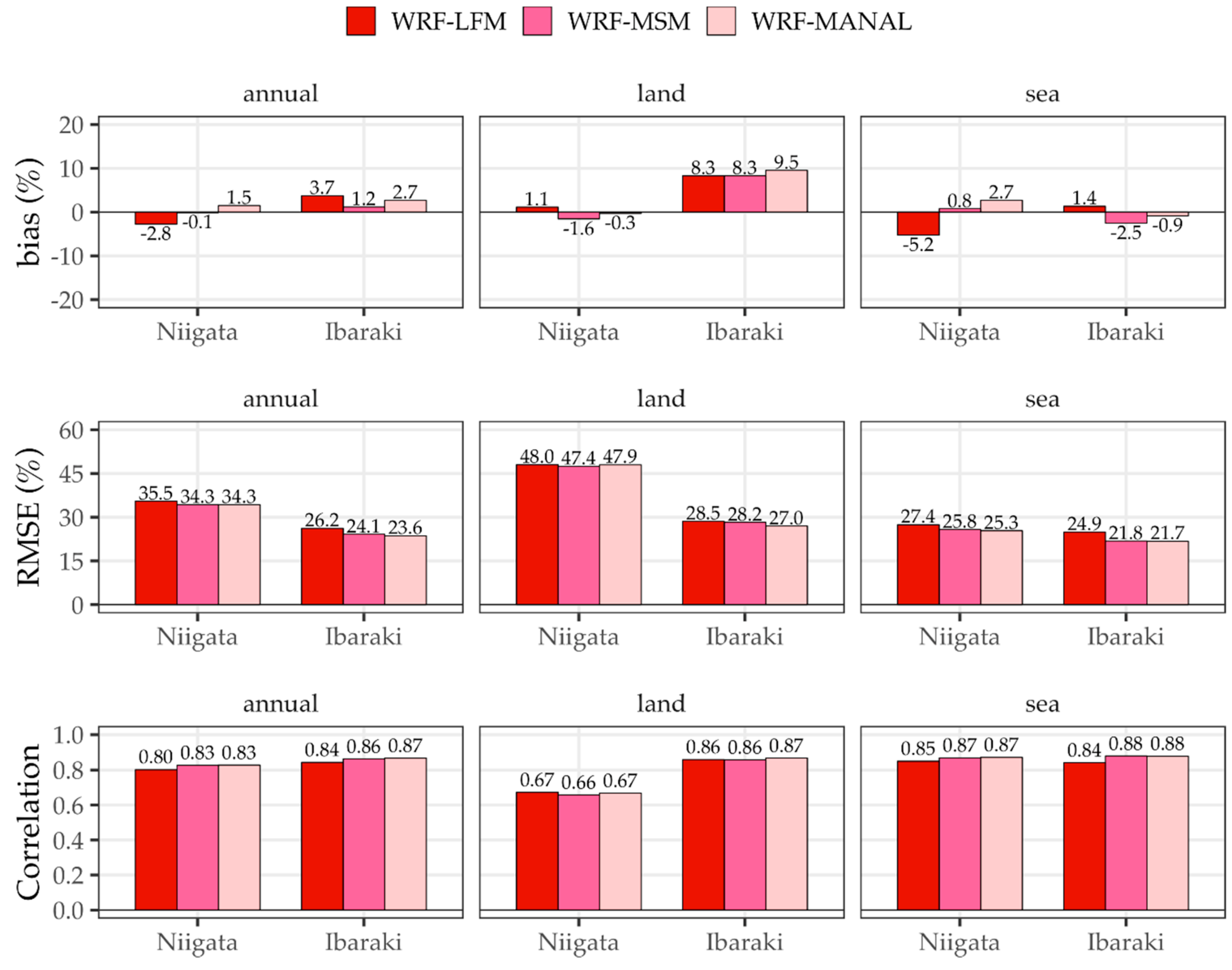
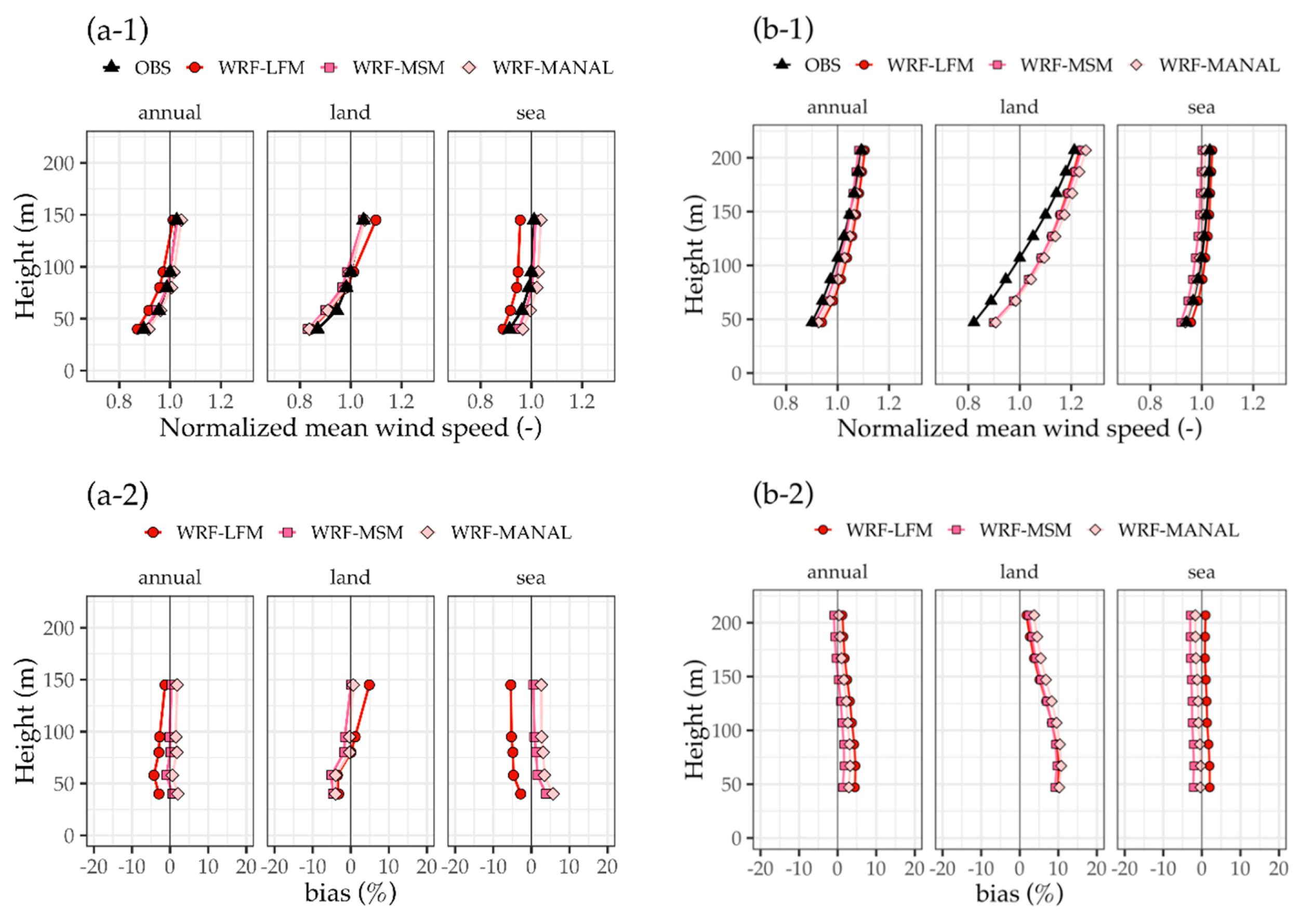
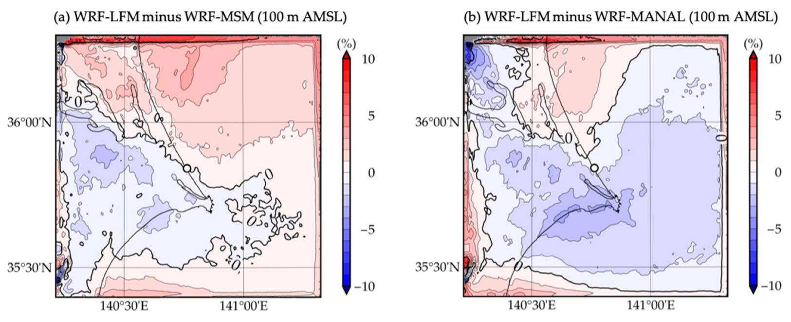
3.3. Comparison between WRF Wind Speeds

As mentioned in the introduction, a primary purpose of this study was to examine whether using the LFM–GPV as the input for the WRF simulation can improve the accuracy of wind speed simulated by WRF. Thus, this subsection describes the sensitivity of the WRF simulations to different input datasets. When focusing on the land-sector wind at Ibaraki, where such an overestimation is typically shown (Figure 6b), it was found that the WRF–LFM exhibited slightly lower wind speeds than the WRF–MSM and WRF–MANAL; however, the differences were slight. Figure 8 shows the spatial distributions of the relative differences between the WRF simulations in the 100-m-height (AMSL) wind speed averaged for the times when the land-sector wind was observed at Ibaraki. Figure 8a,b show the values of the WRF–LFM minus those of the WRF–MSM and those of the WRF–LFM minus those of the WRF–MANAL, respectively. From both figures, it is found that the differences were primarily approximately ±2% over land except for the vicinity of the lateral boundaries; further, the negative values, indicating WRF–LFM < WRF–MSM/WRF–MANAL, encompass larger parts of the land. These results suggest that the LFM–GPV can facilitate a reduction of the tendency of WRF to overestimate the wind speed over land as compared to the other GPVs; however, the effect is limited and is insufficient for a complete improvement.

The WRF–LFM exhibits another problem for the sea-sector wind at Niigata, as shown in Figure 6a-2. The WRF–LFM is found to shift the bias profile toward the negative direction as compared to the WRF–MSM and WRF–MANAL. Figure 9a shows the spatial distributions of relative differences between the WRF–LFM and WRF–MSM simulations at the 100 m height (AMSL) for wind speeds averaged for the times when the sea-sector wind was observed at Niigata: WRF–LFM minus WRF–MSM. Negative values prevail, indicating WRF–LFM < WRF–MSM in the entire domain. To examine the magnitude relationship among the GPVs, the values of LFM–GPV minus MSM–GPV are shown in Figure 9b. The map covers the outer domain of the WRF simulations. As shown in this figure, large negative values over land prevail, and negative values are shown over the sea in the inner domain of WRF. That is, the LFM–GPV exhibits remarkably lower wind speeds than the MSM–GPV in the WRF simulation domains, when the wind blows from the sea sector at Niigata. Considering the model configuration (Table 4), the tendency of the WRF–LFM to underestimate the sea-sector wind speed is likely to be caused by the grid nudging of the low wind speeds of the LFM–GPV in the WRF simulations.

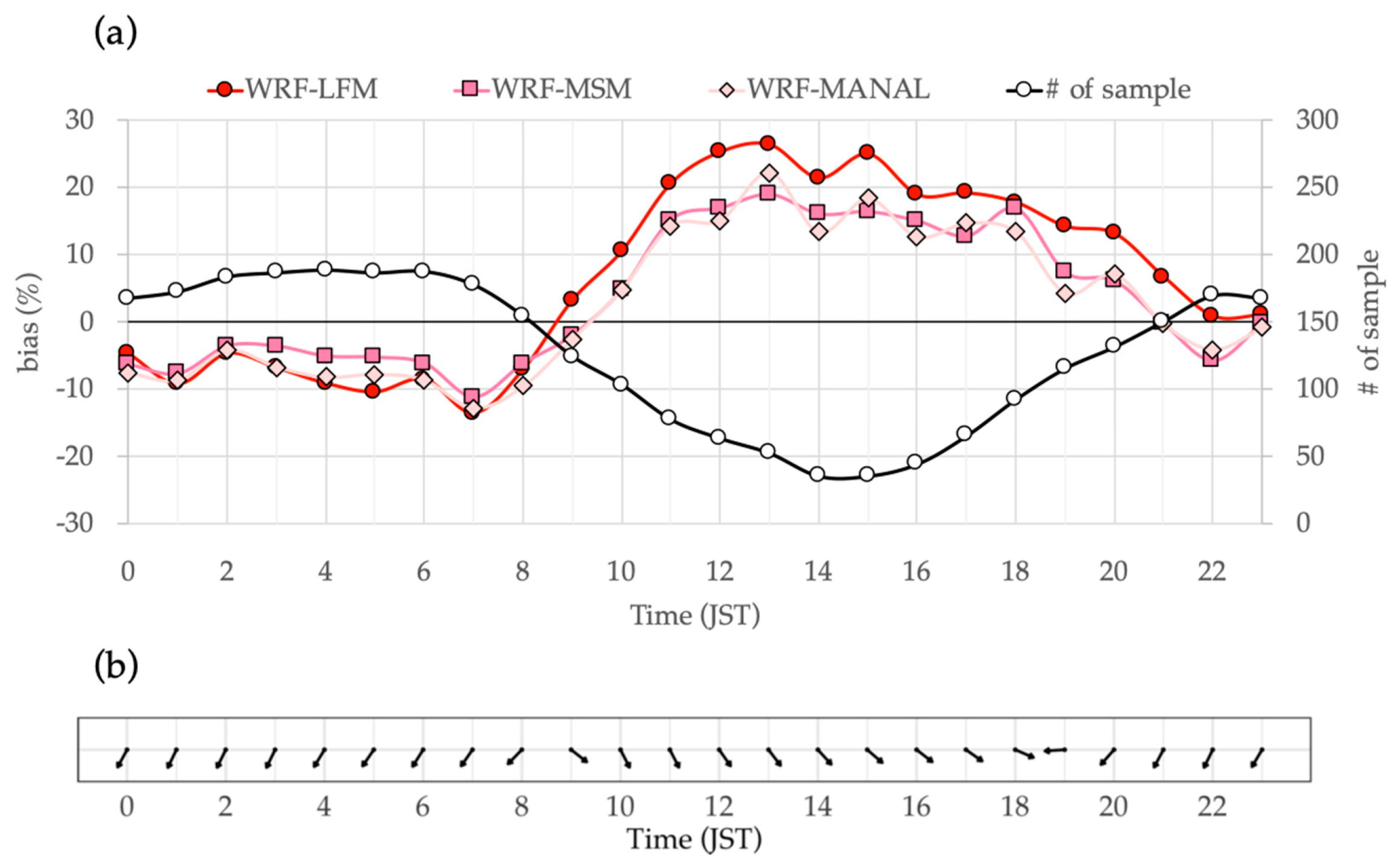
4. Discussion on Overestimation for Wind Speeds over Land

The accuracy comparisons in the previous section indicate that the LFM–GPV exhibited a higher accuracy in wind speed at the two coastal sites, compared to the MSM–GPV and MANAL. It was also shown that the WRF dynamical downscaling simulation using GPVs as input can improve the accuracy of the coastal wind speeds, as compared to the original GPVs. However, it is surprising to find that even if the LFM–GPV, exhibiting the highest accuracy of the three, was used for the WRF simulation, the WRF–LFM simulation did not clearly exhibit more accurate wind speeds than those using the other two GPVs. This result may be interpreted as follows: The effectiveness of using the LFM–GPV is obscured by the tendency of WRF to overestimate the wind speed over land (i.e., the land-sector wind speed in the previous section). In other words, it may be difficult to demonstrate the effectiveness of using the LFM–GPV in the WRF simulation, unless the WRF’s overestimation tendency is improved. Actually, such an observation tendency can lead to an overestimation of the capacity factor of wind turbines, and consequently, to design an unprofitable layout of wind farms. In addition, a similar overestimation tendency was reported in previous studies [11,35,36,37]. Shimada et al. (2011a [35]; 2011b [36]) showed the tendency of WRF to overestimate wind speeds in the PBL over land. Draxl et al. (2014) [37] indicated that the wind speeds simulated by WRF primarily exhibit positive biases at typical wind turbine heights in onshore areas. Kato et al. (2017) [11] speculated that the positive bias in coastal waters was caused by the advection of overestimated wind speeds from land, by demonstrating that the magnitude of the positive bias depends on the fetch from the coast. Thus, to obtain a method to reduce the overestimation, sensitivity simulations with different FDDA (nudging) options and PBL schemes were performed and the possible causes of overestimation are discussed.

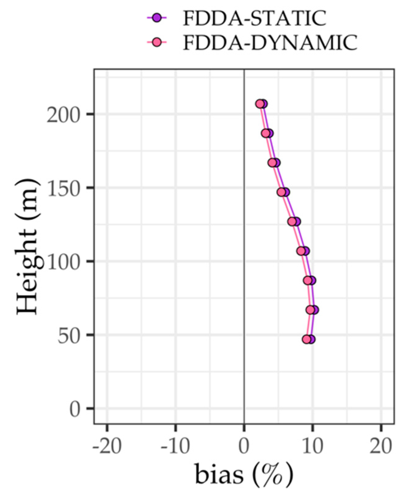
4.1. Effect from Nudging Method

Grid nudging is an FDDA technique that bridges the gap between the model simulations and large-scale meteorological conditions provided from the input data. In the WRF dynamical downscaling simulation for wind resource assessments, the nudging method has frequently been used in previous studies (e.g., [16,35,36,37]).

In WRF, the grid nudging of an arbitrary physical variable, which can be the horizontal component of the wind speed (u, v), potential temperature (θ), or water vapor mixing ratio (q), is implemented by adding an additional tendency term to the nudged variable’s equation as follows:

$$\frac{\partial p*\alpha }{\partial t}=F\left(\alpha ,x,t\right)+G_{\alpha }\cdot W(x,t)\cdot \epsilon \left(x\right)p*\left({\widehat{\alpha }}_0-\alpha \right),$$

(4)

where $p*\alpha$ is the flux from of variable $\alpha$, and the dry column pressure, $p*=p_s-p_t$; $p_s$, is the surface pressure, and $p_t$ is the constant pressure at the top of the model. $F\left(\alpha ,x,t\right)$ is the physical forcing term, where x is the independent spatial variable and t is time. $G_{\alpha }$ is a timescale controlling the nudging strength applied to variable $\alpha \left(G_{\alpha }=1/t’\right)$ and is the nudging timescale. $W$ represents the spatial and temporal weighting, where $W=w_{xy}{w}_{\sigma }{w}_t$. The analysis quality factor, $\epsilon$, ranging between 0 and 1, is based on the quality and distribution of the data used to produce the gridded analysis. ${\widehat{\alpha }}_0$ is the observation analyzed to the grid and interpolated linearly in time.

For the simulations in this study (Table 4), the nudging coefficient, which corresponds to the nudging strength, is set to 0.0003 s⁻¹ as the WRF default. Grid nudging is enabled for the entire outer domain, while it is excluded in the PBL in the inner domain; this method is called FDDA–DYNAMIC in this study. Specifically, the characteristic of FDDA–DYNAMIC is that the nudging space varies dynamically in response to the PBL height; that is, as the PBL becomes higher, the effect of nudging decreases accordingly in the inner domain, and vice versa. To be compared with the FDDA–DYNAMIC, another simulation is performed with an FDDA method, in which the nudging for the outer domain is the same as that for FDDA–DYNAMIC; however, for the inner domain, FDDA is excluded within the PBL defined below a specified height (set to 1500 m AGL in this study). This study refers to this method as FDDA–STATIC. These FDDA–DYNAMIC and FDDA–STATIC simulations were conducted and evaluated for the land-sector wind speeds at Ibaraki, as shown in Figure 6b-2.

Figure 10 shows the vertical profiles of the bias in mean wind speeds for the land sector at Ibaraki, derived from the two WRF–MSM simulations using FDDA–DYNAMIC and FDDA–STATIC. No major differences are shown between the two simulations. A similar result was obtained in the spatial distribution of the relative difference between both nudging simulations in the 100 m height (AMSL) wind speed (not shown). It was therefore concluded that the tendency of WRF to overestimate the wind speed over land is not attributed to the FDDA–DYNAMIC used in Section 3.

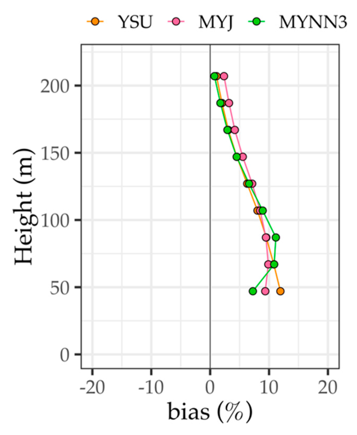
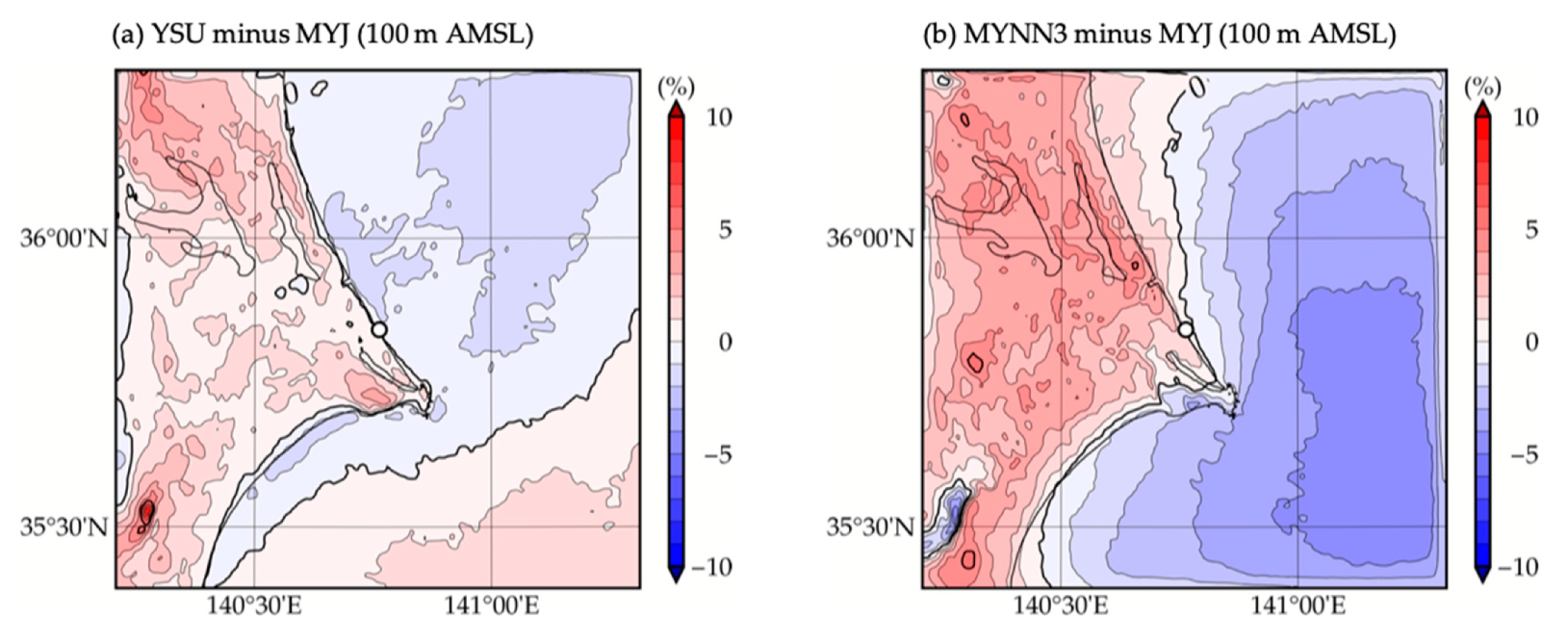
4.2. Effect from PBL Scheme

Next, to identify the sensitivity of the overestimated wind speed over land to the PBL scheme, further WRF simulations were conducted using different PBL schemes. Hu et al. (2006) [38] demonstrated that a positive bias is clearly found only when using the MYJ scheme; Floors et al. (2013) [39] demonstrated that the WRF simulations with different PBL schemes based on the first- and higher-order closure models performed differently for wind directions in the Danish coast. The results of both previous studies indicated that the choice in PBL scheme could affect the accuracy of onshore wind simulations. Thus, in this study, we conducted WRF–MSM simulations with the two different PBL schemes: The first-order Yonsei University (YSU) scheme (Hong et al., 2006 [40]) and the second-order Mellor–Yamada–Nakanishi–Niino Level-3 (MYNN3) scheme (Nakanishi et al., 2006 [41]).

Figure 11 shows the vertical profiles of the bias for the land-sector wind at Ibaraki, derived from the WRF–MSM simulations with the YSU, MYJ, and MYNN3 schemes. No significant differences are indicated among the three simulations, and all of them shows that the positive bias increases in the downward direction. Figure 12 shows the spatial distribution of the relative difference among them in the 100 m height (AMSL) wind speed averaged for the times when the land-sector wind was observed at Ibaraki. Figure 12a,b shows the values of YSU minus MYJ and those of MYNN3 minus MYJ, respectively. Focusing on the land area, positive values prevail in both figures, although the latter exhibit larger values up to approximately 5%. This implies that the wind speeds derived from the YSU and MYNN3 schemes were higher than those from the MYJ scheme. Therefore, we conclude that WRF tends to overestimate the land-sector wind (i.e., wind blowing over land) regardless of the choice in PBL scheme.

4.3. Other Possible Causes

The previous subsections indicated that WRF’s tendency to overestimate the wind speed over land cannot be improved by only changing the nudging methods and PBL schemes. In other words, WRF’s overestimation tendency appears to be attributed to other dynamic or thermodynamic causes in the simulation. It is thus necessary to verify any processes in the surface layer and PBL that can cause the overestimation of the wind speed over land. This final subsection discusses the possible causes of the overestimation, reviewing relevant studies in the past.

From a dynamical point of view, Hahmann et al. (2015) [6] reported that the displacement height and surface roughness length are not considered sufficiently over land in the WRF simulation. Floors et al. (2013) [39] and Varquez et al. (2014) [42] demonstrated that the correction of surface parameters based on observations could improve the accuracy of the wind conditions in WRF simulation. Shimada et al. (2015) [33] suggested using the topo-wind option (Jimenez and Dudhia, 2012 [43]) that considers an additional surface drag owing to unresolved subgrid-scale topography in the momentum equation, to reduce the surface wind speed over complex terrains. However, because this option is adjusted to the domain with a horizontal resolution of 2 km at the highest as the WRF default [43], it cannot be used directly for a high-resolution simulation as that adopted in this study.

Meanwhile, from a thermodynamical point of view, it was reported that WRF overestimates the downward shortwave radiation during the day owing to the underestimation of cloud fraction (Ruiz-Arias et al., 2016 [44]; Shimada et al., 2012 [45]). Because the downward shortwave radiation generally forces the atmospheric stability to be destabilized, and consequently increases the surface wind speed (Mahrt, 1981 [46]), it could be a major cause of the overestimated wind speed over land. In fact, Ruiz-Arias et al. (2016) [44] reported that in the WRF simulation of the Cantabrian Mountains in Spain, the bias in the downward shortwave was decreased partially using the Kain–Frisch (KF) scheme (Kain, 2004 [47]) as a cumulus parameterization together with the subgrid-scale cumulus cloud feedback option (Alapaty et al., 2012 [48]). For a high-resolution simulation, such as that in this study, the new multiscale KF scheme (Zheng et al., 2016 [49]), developed for a higher-resolution simulation (1–10 km) and available since WRF version 3.7 may be useful for increasing the cloud fraction and consequently improving the overestimation tendency of the wind speed over land. In particular, it is worth applying the new scheme to the outer (2.5 or 1.5 km grids) domain.

As a future study, the authors will attempt to improve the tendency of WRF to overestimate the wind speed over land, by considering the following solutions to the three possible causes mentioned above: (1) Re-evaluation of surface roughness (roughness length and zero-plane displacement), (2) introduction of subgrid-scale topographic drag, and (3) improvement in overestimated shortwave radiation.

5. Conclusions

To evaluate whether the WRF simulation forced by the LFM–GPV can provide more accurate wind speeds in coastal areas as compared to those forced by the MSM–GPV and MANAL, we investigated the accuracy of wind speeds derived from the three datasets and the WRF simulations forced by them in comparison with wind lidar measurements at two coastal sites in Japan. The primary conclusions obtained in this study are summarized as follows:

• From the accuracy comparisons between the three JMA datasets, the LFM–GPV exhibited the most accurate wind speeds at the heights from 40 to 200 m. This result is the same as that of our previous study [23], which examined only the surface wind speed, and is reasonable as the LFM–GPV has a higher spatio–temporal resolution than the other datasets.
• The dynamical downscaling simulations with WRF were performed, and we found that the WRF simulations yielded more accurate wind speeds than the input datasets. This was attributed to the ability of WRF to mitigate the negative biases found in the input datasets, especially for the winds blowing from the sea sectors.
• However, we discovered that although the LFM–GPV exhibited the highest accuracy, using the LFM–GPV as an input did not always yield the most accurate wind speeds in the WRF simulation. This was primarily owing to the tendency of WRF to overestimate the wind speed over land that consequently obscured the high accuracy of the LFM–GPV.
• Moreover, it was shown that the overestimation tendency could not be improved by only changing the nudging methods or PBL schemes in the WRF simulation. These results indicated that it may be difficult to utilize the LFM–GPV in the WRF wind simulation, unless the overestimation tendency of WRF is improved first.

References

1. NEDO. The NEDO Offshore Wind Information System. Available online: http://app10.infoc.nedo.go.jp/Nedo_Webgis/top.html (accessed on 29 June 2019).
2. Skamarock, W.; Klemp, J.; Dudhia, J.; Gill, D.; Barker, D.; Duda, M.; Huang, X.; Wang, W.; Powers, J. A description of the advanced research WRF version 3. NCAR Tech. Note NCAR/TN-475+ STR. 2008. [Google Scholar]
3. Sempreviva, A.M.; Barthelmie, R.J.; Pryor, S.C. Review of methodologies for offshore wind resource assessment in European seas. Surv. Geophys. 2008, 29, 471–497. [Google Scholar] [CrossRef]
4. Jimenez, B.; Durante, F.; Lange, B.; Kreutzer, T.; Tambke, J. Offshore wind resource assessment with WAsP and MM5: Comparative study for the German Bight. Wind Energy 2007, 10, 121–134. [Google Scholar] [CrossRef]
5. Peña, A.; Hahmann, A.; Hasager, C.; Bingöl, F.; Karagali, I.; Badger, J.; Badger, M.; Clausen, N. South Baltic Wind Atlas. Available online: http://www.southbaltic-offshore.eu/reports-studies/img/SBO_Wind-Atlas.pdf (accessed on 29 June 2019).
6. Hahmann, A.N.; Lennard, C.; Badger, J.; Vincent, C.L.; Kelly, M.C.; Volker, P.J.; Argent, B.; Refslund, J. Mesoscale modeling for the Wind Atlas of South Africa (WASA) project. DTU Wind Energy 2014, 50, 80. [Google Scholar]
7. Chang, R.; Zhu, R.; Badger, M.; Hasager, C.B.; Xing, X.; Jiang, Y. Offshore wind resources assessment from multiple satellite data and WRF modeling over South China Sea. Remote Sens. 2015, 7, 467–487. [Google Scholar] [CrossRef]
8. Mattar, C.; Borvarán, D. Offshore wind power simulation by using WRF in the central coast of Chile. Renew. Energy 2016, 94, 22–31. [Google Scholar] [CrossRef]
9. Ohsawa, T.; Kozai, K.; Nakamura, S.; Kawaguchi, K.; Shimada, S.; Takeyama, Y.; Kogaki, T. Accuracy of WRF simulation in the NEDO offshore wind resource map. Proc. Jpn. Wind Energy Symp. 2016, 38, 17–20. (In Japanese) [Google Scholar]
10. Ohsawa, T.; Uede, H.; Misaki, T.; Kato, M. Accuracy of WRF Simulations Used for Japanese Offshore Wind Resource Maps. International Conference on Energy and Meteorology 2017. Available online: http://www.wemcouncil.org/ICEMs/ICEM2017_PRES/ICEM_20170629_1120_Sala_2_Ohsawa.pptx (accessed on 29 June 2019).
11. Kato, M.; Ohsawa, T.; Uede, H.; Shimada, S. Verification of spatial characteristics of WRF-simulated wind speed in Japanese coastal waters. Proc. Jpn. Wind Energy Symp. 2017, 39, 253–256. (In Japanese) [Google Scholar]
12. Hong, S.Y.; Dudhia, J. Next-generation numerical weather prediction: Bridging parameterization, explicit clouds, and large eddies. Bull. Am. Meteorol. Soc. 2012, 93, ES6–ES9. [Google Scholar] [CrossRef]
13. Carvalho, D.; Rocha, A.; Gómez-Gesteira, M. Ocean surface wind simulation forced by different reanalyses: Comparison with observed data along the Iberian Peninsula coast. Ocean Model. 2012, 56, 31–42. [Google Scholar] [CrossRef]
14. Carvalho, D.; Rocha, A.; Gómez-Gesteira, M.; Santos, C.S. Offshore wind energy resource simulation forced by different reanalyses: Comparison with observed data in the Iberian Peninsula. Appl. Energy 2014, 134, 57–64. [Google Scholar] [CrossRef]
15. Carvalho, D.; Rocha, A.; Gómez-Gesteira, M.; Santos, C.S. WRF wind simulation and wind energy production estimates forced by different reanalyses: Comparison with observed data for Portugal. Appl. Energy 2014, 117, 116–126. [Google Scholar] [CrossRef]
16. Hahmann, A.N.; Vincent, C.L.; Peña, A.; Lange, J.; Hasager, C.B. Wind climate estimation using WRF model output: Method and model sensitivities over the sea. Int. J. Climatol. 2015, 35, 3422–3439. [Google Scholar] [CrossRef]
17. Chadee, X.T.; Seegobin, N.R.; Clarke, R.M. Optimizing the Weather Research and Forecasting (WRF) Model for Mapping the Near-Surface Wind Resources over the Southernmost Caribbean Islands of Trinidad and Tobago. Energies 2017, 10, 931. [Google Scholar] [CrossRef]
18. JMBSC. MANAL. Available online: http://www.jmbsc.or.jp/jp/offline/cd0380.html (accessed on 29 June 2019).
19. Akimoto, Y.; Kusaka, H. Sensitivity of the WRF Regional Meteorological Model to Input Datasets and Surface Parameters for the Kanto Plain on Fine Summer Days. Geogr. Rev. Jpn. Ser. A 2010, 83, 324–340. (In Japanese) [Google Scholar] [CrossRef] [Green Version]
20. NCEP. FNL Operational Model Global Tropospheric Analyses, Continuing from July 1999. Available online: https://doi.org/10.5065/D6M043C6 (accessed on 29 June 2019).
21. JMBSC. LFM-GPV. Available online: http://www.jmbsc.or.jp/jp/online/file/f-online10300.html (accessed on 29 June 2019).
22. JMBSC. MSM-GPV. Available online: http://www.jmbsc.or.jp/jp/online/file/f-online10200.html (accessed on 29 June 2019).
23. Misaki, T.; Ohsawa, T. Evaluation of LFM-GPV and MSM-GPV as input data for wind simulation. J. Jpn. Wind Energy Assoc. 2019, 42, 72–79. [Google Scholar]
24. ZephIR Lidar. ZephIR 300. Available online: https://s.campbellsci.com/documents/ca/product-brochures/zephir300_br.pdf (accessed on 29 June 2019).
25. Gottschall, J.; Courtney, M. Verification Test for Three WindCube WLS7 LiDARs at the Høvsøre Test Site; Danmarks Tekniske Universitet, Risø Nationallaboratoriet for Bæredygtig Energi: Roskilde, Denmark, 2010. [Google Scholar]
26. PARI. Hazaki Oceanographical Research Station (HORS). Available online: https://www.pari.go.jp/unit/edosy/en/main-facility/2.html (accessed on 29 June 2019).
27. Mito, T.; Kato, H.; Konagaya, M.; Matsuoka, Y. Accuracy comparison between multiple models of vertical wind Doppler LIDAR. Proc. Jpn. Wind Energy Symp. 2016, 38, 209–211. (In Japanese) [Google Scholar]
28. Shimada, S.; Takeyama, Y.; Kogaki, T.; Ohsawa, T.; Nakamura, S. Investigation of the fetch effect using onshore and offshore vertical LIDAR devices. Remote Sens. 2018, 10, 1408. [Google Scholar] [CrossRef]
29. JMA. Joint WMO Technical Progress Report on the Global Data Processing and Forecasting System and Numerical Weather Prediction Research Activities for 2016. Available online: http://www.jma.go.jp/jma/jma-eng/jma-center/nwp/report/2016_Japan.pdf (accessed on 29 June 2019).
30. NLNI. Land Utilization Segmented Mesh Data. Available online: http://nlftp.mlit.go.jp/ksj-e/jpgis/datalist/KsjTmplt-L03-b.html (accessed on 29 June 2019).
31. Sertel, E.; Robock, A.; Ormeci, C. Impacts of land cover data quality on regional climate simulations. Int. J. Climatol. 2010, 30, 1942–1953. [Google Scholar] [CrossRef]
32. Tewari, M.; Chen, F.; Wang, W.; Dudhia, J.; LeMone, M.A.; Mitchell, K.; Ek, M.; Gayno, G.; Wegiel, J.; Cuenca, R.H. Implementation and verification of the unified NOAH land surface model in the WRF model. In Proceedings of the 20th Conference on Weather Analysis and Forecasting/16th Conference on Numerical Weather Prediction, Seattle, WA, USA, 10–15 January 2004; pp. 11–15. [Google Scholar]
33. Shimada, S.; Ohsawa, T.; Kogaki, T.; Steinfeld, G.; Heinemann, D. Effects of sea surface temperature accuracy on offshore wind resource assessment using a mesoscale model. Wind Energy 2015, 18, 1839–1854. [Google Scholar] [CrossRef]
34. Janjić, Z.I. The step-mountain eta coordinate model—Further developments of the convection, viscous sublayer, and turbulence closure schemes. Mon. Weather Rev. 1994, 122, 927–945. [Google Scholar] [CrossRef]
35. Shimada, S.; Ohsawa, T. Accuracy and characteristics of offshore wind speeds simulated by WRF. SOLA 2011, 7, 21–24. [Google Scholar] [CrossRef]
36. Shimada, S.; Ohsawa, T.; Chikaoka, S.; Kozai, K. Accuracy of the wind speed profile in the lower PBL as simulated by the WRF model. SOLA 2011, 7, 109–112. [Google Scholar] [CrossRef]
37. Draxl, C.; Hahmann, A.N.; Peña, A.; Giebel, G. Evaluating winds and vertical wind shear from Weather Research and Forecasting model forecasts using seven planetary boundary layer schemes. Wind Energy 2014, 17, 39–55. [Google Scholar] [CrossRef]
38. Hu, X.M.; Nielsen-Gammon, J.W.; Zhang, F. Evaluation of three planetary boundary layer schemes in the WRF model. J. Appl. Meteorol. Climatol. 2010, 49, 1831–1844. [Google Scholar] [CrossRef]
39. Floors, R.; Vincent, C.L.; Gryning, S.E.; Peña, A.; Batchvarova, E. The wind profile in the coastal boundary layer: Wind lidar measurements and numerical modelling. Boundary-Layer Meteorol. 2013, 147, 469–491. [Google Scholar] [CrossRef]
40. Hong, S.Y.; Noh, Y.; Dudhia, J. A new vertical diffusion package with an explicit treatment of entrainment processes. Mon. Weather Rev. 2006, 134, 2318–2341. [Google Scholar] [CrossRef]
41. Nakanishi, M.; Niino, H. An improved Mellor-Yamada Level-3 model: Its numerical stability and application to a regional prediction of advection fog. Boundary-Layer Meteorol. 2006, 119, 397–407. [Google Scholar] [CrossRef]
42. Varquez, A.C.G.; Nakayoshi, M.; Makabe, T.; Kanda, M. WRF Application of High Resolution Urban Surface Parameters on Some Major Cities of Japan. J. Jpn. Soc. Civil Eng. Ser. B1 (Hydraul. Eng.) 2014, 170, I_175–I_180. [Google Scholar] [CrossRef]
43. Jimenez, P.A.; Dudhia, J. Improving the representation of resolved and unresolved topographic effects on surface wind in the WRF model. J. Appl. Meteorol. Climatol. 2012, 51, 300–316. [Google Scholar] [CrossRef]
44. Ruiz-Arias, J.A.; Arbizu-Barrena, C.; Santos-Alamillos, F.J.; Tovar-Pescador, J.; Pozo-Vázquez, D. Assessing the surface solar radiation budget in the WRF model: A spatiotemporal analysis of the bias and its causes. Mon. Weather Rev. 2016, 144, 703–711. [Google Scholar] [CrossRef]
45. Shimada, S.; Liu, Y.Y.; Xia, H.; Yoshino, J.; Kobayashi, T.; Itagaki, A.; Utsunomiya, T.; Hashimoto, J. Accuracy of solar irradiance simulation using the WRF-ARW model. J. Jpn. Sol. Energy Soc. 2012, 38, 41–48. (In Japanese) [Google Scholar]
46. Mahrt, L. The early evening boundary layer transition. Q. J. R. Meteorol. Soc. 1981, 107, 329–343. [Google Scholar] [CrossRef]
47. Kain, J.S. The Kain–Fritsch convective parameterization: An update. J. Appl. Meteorol. 2004, 43, 170–181. [Google Scholar] [CrossRef]
48. Alapaty, K.; Herwehe, J.A.; Otte, T.L.; Nolte, C.G.; Bullock, O.R.; Mallard, M.S.; Kain, J.S.; Dudhia, J. Introducing subgrid-scale cloud feedbacks to radiation for regional meteorological and climate modeling. Geophys. Res. Lett. 2012, 39. [Google Scholar] [CrossRef]
49. Zheng, Y.; Alapaty, K.; Herwehe, J.A.; Del Genio, A.D.; Niyogi, D. Improving high-resolution weather forecasts using the Weather Research and Forecasting (WRF) model with an updated Kain–Fritsch scheme. Mon. Weather Rev. 2016, 144, 833–860. [Google Scholar] [CrossRef]
Figure 1. Maps of (a) the whole of Japan and the domains used in the WRF simulation for the observation sites of (b) Niigata and (c) Ibaraki. Background color represents terrain height in meters. Red dots and lines denote the lidar observation sites and directions to separate the land and sea sectors, respectively.
Energies 12 02754 g001
Figure 2. Wind roses (a) at Niigata (95 m) and (b) at Ibaraki (107 m). Colors denote the appearance frequencies of wind-speed classes.
Energies 12 02754 g002
Figure 3. Biases, RMSEs, and correlation coefficients for mean wind speeds derived from LFM–GPV, MSM–GPV, and MANAL for the whole year (annual), at the land sector (land), and at the sea sector (sea) at Niigata (95 m) and Ibaraki (107 m).
Energies 12 02754 g003
Figure 4. Vertical profiles of (1) mean wind speeds derived from the observation and LFM–GPV, MSM–GPV, and MANAL and (2) their biases, for the whole year (annual), the land sector (land), and the sea sector (sea), at (a) Niigata and (b) Ibaraki. The mean wind speeds are normalized by each of corresponding mean wind speeds observed at a 95 m height at Niigata and at a 107 m height at Ibaraki, whereas the biases are normalized by the observed mean wind speed at each height.
Energies 12 02754 g004aEnergies 12 02754 g004b
Figure 5. Similar to Figure 3, but for wind speeds derived from WRF–LFM, WRF–MSM, and MANAL simulations.
Energies 12 02754 g005
Figure 6. Similar to Figure 4, but for wind speeds derived from WRF–LFM, WRF–MSM, and MANAL simulations.
Energies 12 02754 g006
Figure 7. Accuracy variations of the WRF wind speed in a day at Niigata: (a) biases of hourly 95 m height wind speeds averaged for land-sector winds, derived from WRF–LFM, WRF–MSM, and WRF–MANAL simulations. The solid black line denotes the number of samples at each time. (b) Appearance frequency of wind direction at each hour, based on lidar observation at 95 m.
Energies 12 02754 g007
Figure 8. Spatial distributions of relative differences (a) between WRF–LFM and WRF–MSM simulations and (b) between WRF–LFM and WRF–MANAL simulations for the 100-m-height (AMSL) wind speed averaged for the times when the land-sector wind is observed at Ibaraki. White dots denote the site of Ibaraki.
Energies 12 02754 g008
Figure 9. Spatial distributions of relative differences between (a) WRF–LFM and WRF–MSM simulations at a 100 m height (AMSL) and (b) LFM–GPV and MSM–GPV at a 10 m height (AGL) for wind speeds averaged for the times when the sea-sector wind is observed at Niigata. White dots denote the site of Niigata and gray color denotes the area with an altitude over 100 m (AMSL) based on terrains of WRF–MSM. A black frame in (b) denotes the inner domain.
Energies 12 02754 g009
Figure 10. Vertical profiles of the biases in mean wind speeds for the land-sector winds at Ibaraki, derived from the two WRF–MSM simulations using FDDA–DYNAMIC and FDDA–STATIC.
Energies 12 02754 g010
Figure 11. Similar to Figure 10, but for wind speeds derived from three WRF–MSM simulations with YSU, MYJ, and MYNN3 schemes.
Energies 12 02754 g011
Figure 12. Spatial distributions of relative differences between two WRF–MSM simulations with (a) YSU and MYJ schemes and (b) MYNN3 and MYJ schemes for the 100 m height (AMSL) wind speed averaged for the times when the land-sector wind was observed at Ibaraki. White dots denote the site of Ibaraki.
Energies 12 02754 g012