Propeller Synchrophasing Control with a Cylindrical Scaled Fuselage Based on an Improved Data Selection Algorithm


1
Jiangsu Province Key Laboratory of Aerospace Power System, Nanjing University of Aeronautics and Astronautics, Nanjing 210016, China
2
AECC Aero Engine Control System Institute, Wuxi 214063, China
*
Author to whom correspondence should be addressed.
Energies 2019, 12(14), 2736; https://doi.org/10.3390/en12142736
Submission received: 21 June 2019
/
Revised: 14 July 2019
/
Accepted: 15 July 2019
/
Published: 17 July 2019
(This article belongs to the Special Issue Recent Advances in Stochastic Methods for Energy Analysis)
Abstract
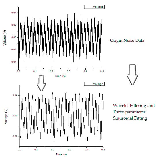
:Propeller synchrophasing control is an active noise control method which can effectively reduce the noise in the cabin of a turboprop aircraft. The propeller signature model identified by the measured acoustic noise data is easily affected by flight speed, altitude, and the existence of the fuselage. Meanwhile, the noise excited by the propellers is nonstationary signal, which often fluctuates greatly, thus affecting the accuracy of the identification of the model. In this paper, a synchrophasing control experimental platform with a cylindrical scaled fuselage on ground is firstly established to validate the actual noise reduction in the cabin. Then, a minimum fluctuation data selection method based on wavelet filtering and three-parameter sinusoidal fitting is proposed to improve the identification accuracy of the propeller signature model. This method extracts the high-precision propeller blade passing frequency signal from the noise signal by using a wavelet filtering algorithm and selects the minimum fluctuation data segment by using a three-parameter sinusoidal fitting algorithm. The experimental results firstly show the significant noise attenuation achieved in the cabin using propeller synchrophasing control. Secondly, the propeller signature model improved by the minimum fluctuation data selection method has higher accuracy than that identified by the traditional method.
1. Introduction
The acoustic noise excited by rotating propellers consists of two parts: rotating noise and broadband noise. Rotational noise is caused by the interaction of the blade with the periodic flow while broadband noise is produced by the random pulsating interaction of the blade with the surrounding flow field [1]. Spectrum characteristics analysis shows that the main component of the cabin noise of turboprop aircraft is the superposition of broadband noise and a series of discrete frequency noise, where the latter section plays a dominant role [2]. When the propellers are rotating steadily, the discrete frequency noise is a long wavelength signal of 100–250 Hz and it is difficult to achieve noise reduction by passive noise control techniques. Also, the propellers need to be rotating at the same rate in order to provide the equivalent thrust and torque on each side to make the plane balanced. It is required that the noise inside the cabin be reduced by 25 dB to reach the level of an equivalent turbofan aircraft [3]. Among various active noise control methods, propeller synchrophasing control is superior to the others in terms of the requirement for no additional sensors or actuators (no additional weight) while providing significant noise reduction [4,5]. The principle of propeller synchrophasing is to maintain a certain phase angle difference which is defined as the optimal phase angle between several propellers of a multipropeller aircraft, so that part of the rotating noise and vibration generated by each propeller cancel each other out, and the cabin noise is minimized.
Blunt et al. [5] carried out synchrophasing control experiments in a real flight on C-130J-30 and AP-3C. Obviously, the cost of the real flight is huge and the experiments are time-consuming, meaning they are not be suitable for further research on propeller synchrophasing control. Huang et al. [6] and Sheng et al. [7] established a ground experimental platform to study the effectiveness of synchrophasing control and significant noise reduction was achieved. However, the existence of the fuselage is an inevitable factor that can affect the performance of the synchrophasing control, and is difficult to analyze due to the complex acoustic vibration couplings between the fuselage and the enclosed cabin space. Investigation needs to be made to explore the real performance of the synchrophasing control inside the cabin in the presence of the fuselage in a relative low-cost way.
Noise modeling is the key issue to achieve significant noise reduction. Experimental and analytical works on the problem of noise modeling have been carried out by several researchers [8]. Atassi et al. [9] determined that the fluctuating loads resulted from ingested turbulence from blade to blade. Ground vortex ingestion was considered in the noise modeling in stationary or near-stationary aircraft engines by Murphy et al. [10]. Stephens et al. [11] studied casing boundary layer/rotor interaction and unsteady blade loading, and the radiated sound was determined by strip theory, where the streamwise velocity component was measured. Martio et al. [12] found that the blade passage frequency (BPF) would oscillate due to the unsteady thrust of the propeller at the highest thrust conditions. Far-field acoustic predictions were made by Glegg et al. [13]. Good agreements were achieved between the predictions and the measurements at low and moderate thrust. The measured undisturbed boundary layer turbulence correlations were adopted in the study. However, these studies focused on the aspect of the fluid dynamics.
Most studies of propeller synchrophasing control are based on propeller signature theory. The optimal phase angle for minimizing noise is predicted by the propeller signature model, which is identified by the noise information of several independent phase angle pairs in the first stage [14,15]. However, the propeller signature model is dynamically influenced by factors such as flight altitude, Mach number, and flight angle of attack, resulting in unexpected inaccuracy of the optimal phase angle [16]. Obtaining the optimal phase angle based on the propeller signature model is the key for propeller noise reduction. The accuracy of the model has a crucial impact on the actual effect of noise attenuation. Therefore, how to establish the high-precision propeller signature model under different flight conditions is a major concern. The measured sound pressure often fluctuates greatly due to the influence of flight speed, altitude, airflow variation, and circuit noise during the acquisition process. In order to reduce the impact of data fluctuations, the common solution is to collect noise information from more phase angles pairs than the required minimum pairs, thereby reducing the impact of unexpected data fluctuation on model accuracy [17,18].
An algorithm for truncating the very beginning and tail of measured noise data is proposed by Huang et al. [6] for minimizing transient data fluctuation caused by noise acquisition start and stop manipulation. The algorithm has obvious effects for some occasions, but the conclusion is made only based on experimental data and the length of the intercepted data lacks theoretical criteria. Another study [19] developed a method to improve the modeling accuracy by changing the number of sampling noise data cycles. It points out that the shorter the sampling time is, the smaller the influence of phase angle fluctuation on the identification accuracy would be. However, if the sampling time is too short, the identified model may lose necessary noise information and random errors would be magnified, thus prediction of the optimal phase angle is not correct. The existing methods for dealing with the data fluctuations are mainly based on experience and experiments and have certain limitations due to the lack of an effective data selection method.
Wavelet analysis is a useful mathematical tool in multiresolution modeling [20] and is often used for complex structural analysis. Belytschko et al. [21] and Zienkiewicz et al. [22] adopted a wavelet-based homogenization method to solve the unidirectional transient problems of heat transfer and free vibrations. The homogenization method based on wavelets gave satisfactory approximation of the real transient processes. The wavelet-based space-time decomposition was proposed by Bacry et al. [23] to model the transient heat transfer process. Literature [24] focused on the problem of finite element method (FEM)-based homogenization using Haar basis to determine the coefficients. Christon et al. [25] used the wavelet decomposition-based finite element method to discretize the composite model. The application of the wavelet analysis can be found in the eigenproblem solution [26], wave propagation [27], wave detection [28], and damage monitoring [29]. Frantziskonis [30] applied the wavelet functions to serve as random process approximations to solve the probabilistic problems in the structural analysis.
In order to improve the accuracy of the propeller signature model, this paper proposes a minimum data fluctuation selection algorithm based on wavelet filtering and a three-parameter sinusoidal fitting method. Wavelet filtering is adopted here to extract low-frequency signals from propeller noise signals, where the dominant signal is the BPF signal. The fluctuation of the BPF signal can directly reflect the propeller noise and phase angle fluctuations. The fluctuation of the measured noise data in whole acquisition period is evaluated by the proposed method and then the data segment with the least fluctuation is selected for modeling. An experimental platform with a cylindrical scaled fuselage is built to validate the real performance of the synchrophasing control inside the cabin and the data selection method.
The paper is organized as follows: the principle of the propeller signature is presented in Section 2. In Section 3, we present the experimental platform with the scaled fuselage and the performance of the synchrophasing control inside the cabin. Section 4 describes the wavelet filtering and the three-parameter sinusoidal fitting method for data selection. Finally, Section 5 summarizes the paper.
2. Propeller Signature Principle
According to the propeller signature theory [17], the propeller noise at a certain position inside the cabin is the vector sum of noise generated by each propeller. When the propeller speeds are synchronized and the phase angle difference remains fixed, the noise can be predicted by the combination of phase angles between the propellers.
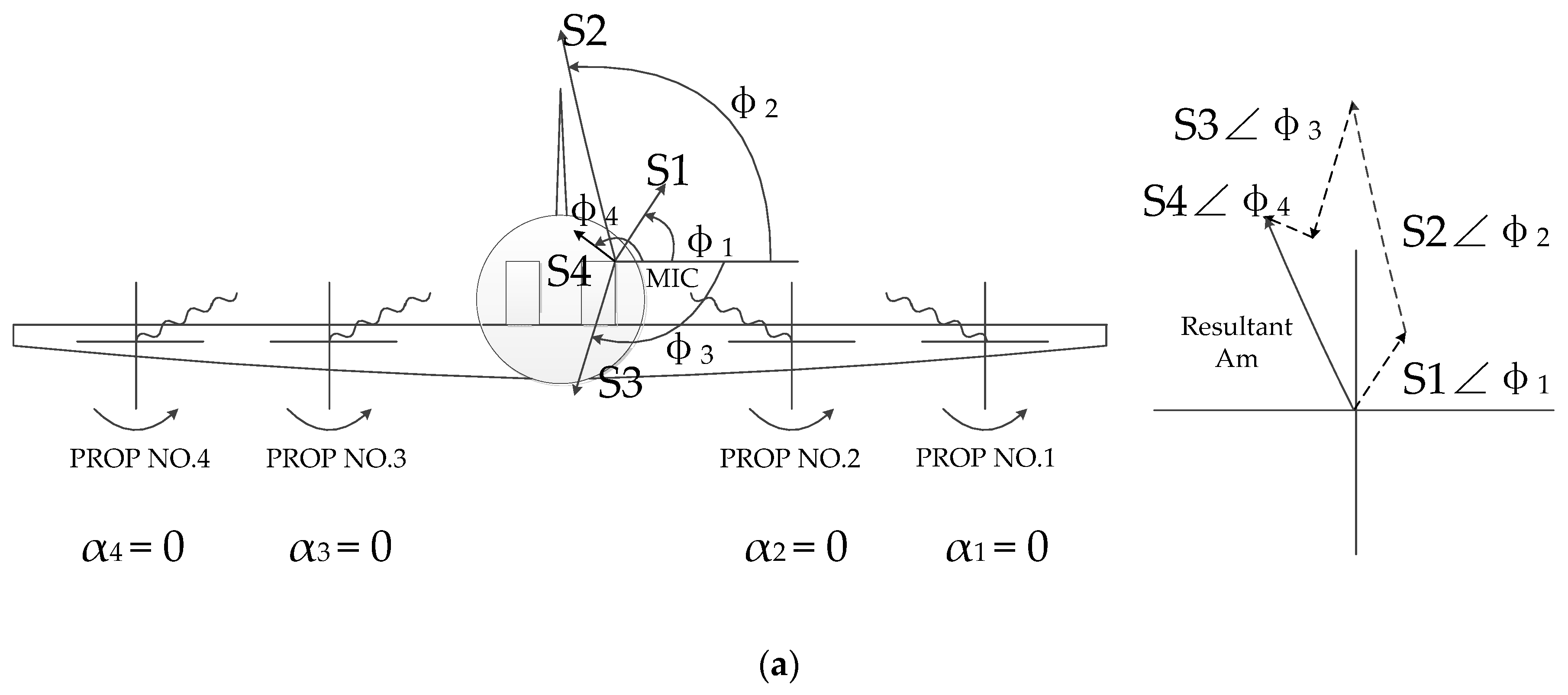
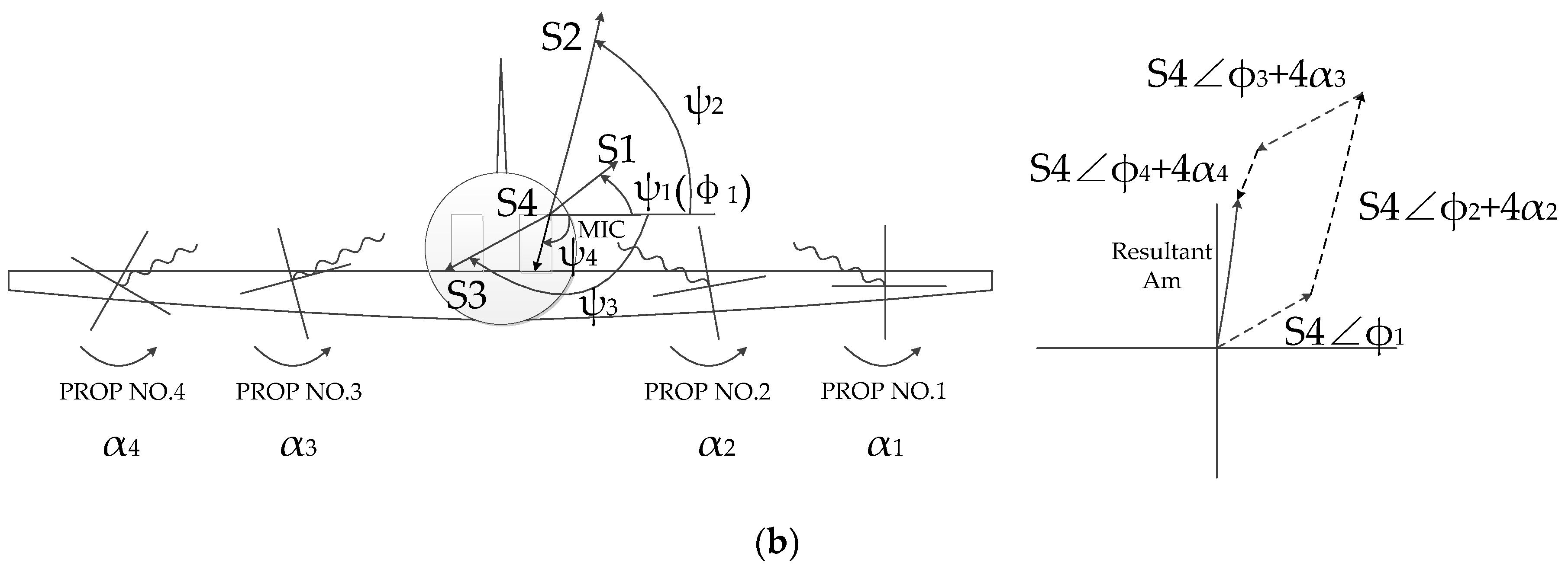
A BPF noise distribution example of the four propeller engines is shown in Figure 1. Assuming at this moment, the propellers running at the same speed are working at the condition in Figure 1a, S1, S2, S3, and S4 are the modulus of the propeller signatures which represent the individual BPF noise contribution from each propeller while the resultant noise Am is the sum of the noise vector from all the contributions forming the ‘final’ BPF noise at the measurement point. For the sake of convenience, No. 1 propeller is defined as the master propeller and the rest as the slave propellers. As the propellers rotate, the angles of the propellers’ blades change. At the moment depicted in Figure 1b, the phase angle pair where not all of them are zero at the same time.
At any moment, the modulus of each propeller will be the same, i.e., S1, S2, S3, and S4 would remain unchanged, but the phase, which is represented as ψ, in the left part of Figure 1b would change as depicted. Note that the propeller signature phase ψ could be expressed as the result of the phase φ when the propeller angle α equals to zero plus the nonzero propeller angle times the blade number B which is four in this case. It can be seen that the resultant noise Am in Figure 1b is smaller than that in Figure 1a, indicating noise reduction at the same observer location. Obviously, among all possible phase angle pairs , there must be one pair resulting in the smallest Am, i.e., the lowest noise, due to the boundedness of the noise level. Similar results describing the same concept above can be found in Figure 3.3 of reference [31]. This phase angle pair is defined as optimal synchrophase angle at the observer location. Propeller synchrophasing control firstly acquires the noise data of different phase angle pairs and then identifies the propeller signature model using the noise data [5]. A previous study [31] gives the contributions at BPF excited by the propellers at a certain location k:
where is the BPF contribution in complex form, is the modulus of the p-th propeller signature at the position k, P indicates the number of propellers, B represents the blade number of the propeller, and is the propeller phase angle. For the multiposition measurement case, the BPF contributions can be written in the following matrix form:
where the definition of parameters is the same as Equation (1). In a simple matrix notion, Equation (2) can also be written as
where is a column vector representing the BPF contribution at different K locations, is a matrix indicating the propeller signatures, and is a column vector representing the phase information of propeller signatures.
Mathematically, to solve in Equation (3), at least the P independent phase angle pairs are required. Usually, more than P pairs are measured to improve the modeling accuracy. For Q pairs measurements (Q > P), the propeller signature can be obtained by the least squares method:
where is the complex conjugate transpose of . This process can be applied to the harmonics of the BPF by replacing of the BPF noise to the n-th order harmonic contributions and changing parameter to . Because the propellers are running at lower speed compared to that of turbofan, the low order harmonic components are in the dominating position in the spectrum analyses, which indicates that the high order harmonics can be neglected when the propeller signature model is identified. Huang et al. [6] takes only the first six orders of the harmonic for the identification and good agreement is achieved between the real noise level and the noise prediction. To determine the accuracy of the model, the first ten harmonics are selected in this paper. Once the propeller signatures are determined, the optimal synchrophase angle can be predicted by changing the synchrophasing angles. The above process can be done offline and when the propellers are working, synchrophasing control maintains the optimal synchrophasing angle to retain the lowest noise level.
The synchrophasing control method can be promoted to other setups where the number of the blades per propeller is different if the BPF frequency is relatively low (less than 250 Hz).
3. Experimental Platform with the Cylindrical Scaled Fuselage
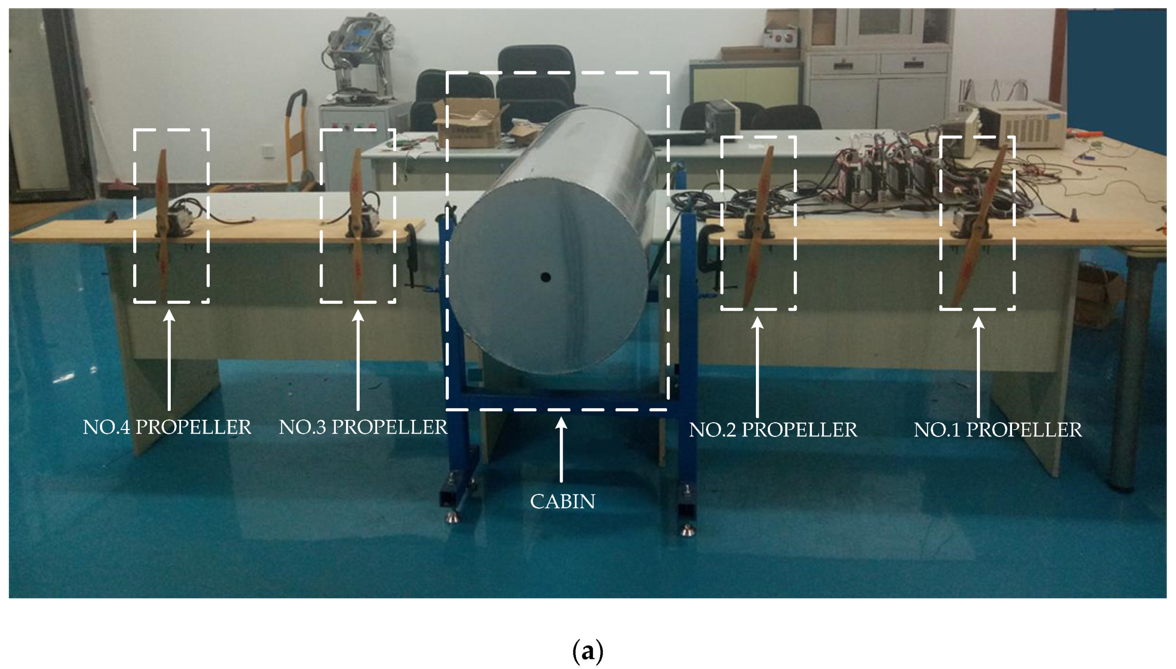
The propeller synchrophasing control experiment can be conducted in real flight and on the ground. However, the huge cost and the inconvenience of real flight testing cannot be neglected. To the best of our knowledge, only a few flight tests have been carried out. Some researchers have conducted ground experiments to validate the performance of propeller synchrophasing control [6,7,18]. The experiments were established in a free acoustic field without the influence of the possible reflection in the presence of the fuselage. In order to validate the performance of propeller synchrophasing control inside the cabin and to deploy other active noise control algorithms in the future, this paper builds a ground test platform with a cylindrical scaled fuselage as shown in Figure 2.
Figure 2a is the overall structure of the ground test platform, where four servo-motors are adopted to drive four rotating propellers to simulate the noise of a four-propeller aircraft. The four propellers are two-blade propellers, numbered 1–4 from the right to the left. In the middle of the four propellers, a thin cylindrical shell is used to simulate the acoustic characteristics of the cabin, which is suggested for ground testing [32]. The cylinder is 1.5 m in length, 0.5 m in diameter, and 2 mm in thickness. It is made of aviation aluminum material. Figure 2b is an internal structure diagram of cylinder fuselage illustrated in the software. The bottom floor made of wood is used to simulate the cabin floor. There are four microphone mounting holes on the microphone mounting arm, numbered 1–4 from right to left as depicted in the figure. The mounting arm can slide and rotate on the slider to measure noise data at multiple locations as far as the microphones can reach. The noise of four different points can be measured simultaneously.
As mentioned in Section 2, for a case of four propellers, at least four independent propeller angle pairs are required to solve Equation (3). This paper selects eight angle pairs which are shown in Table 1 for the identification. Noise data over 10 s for each pair are measured by four microphones.
Note that 0.125 s or one second length measurement noise are often used to calculate the sound pressure level (SPL) in commercial noise measurement instruments. When the real-time requirement of SPL is high, the noise data of 0.125 s is used to calculate SPL; that is to say, SPL is evaluated every 0.125 s, which is similar to the physiological characteristics of human hearing [33]. When the accuracy requirement of SPL is high, one second noise data is usually used to calculate SPL. In order to improve the accuracy of the propeller signature model as much as possible, the middle part (4–5 s) of the raw 10 s measurement is chosen for the calculation in this section. Apart from that, if the sampling frequency is 44,100 Hz, the noise data of 1 s contains the first ten harmonics of the noise, where the frequency of the 10th harmonic is 500 Hz when a two-blade propeller is running at 1500 resolutions per minute (RPM). Thus, one second length noise data can provide sufficient harmonic information.
The phase angles of propellers No. 1, No. 3, and No. 4 are set to be zero throughout the experiment. The phase angle of propeller No. 2 is set to start from zero and increase by 5 degrees every 10 s until the phase angle becomes 180 degrees. The rotational speed of the No. 2 propeller is set to be fixed at 1500 RPM when the reference angle is met and during the settlement period of the new phase angle, only is added to 1500 RPM as the bias. The rotational speed of the other propellers is controlled at 1500 RPM throughout the experiment. The microphone installation arm is positioned to be horizontal and is moved to the rear region inside the fuselage in the experiment.
The results are shown in Figure 3. The black line in the figure represents the actual noise level at the observer location and the red line represents the noise predicted by the propeller signature model. The noise was firstly recorded by the microphones at different locations. Then, FFT transform was applied to the recorded data; thus, the BPF signal and its harmonics were obtained. Propeller signatures of different harmonic orders (first ten orders in this paper) were solved using Equation (4) by changing and with the corresponding harmonic amplitudes and phase information, respectively. Once the propeller signatures of first ten harmonic orders were acquired, the resultant noise level at the specific location was calculated by changing the phase angle (only α2 changed; α1, α3, and α4 remain unchanged) of in Equation (2). A more detailed process can be found in the literature [6] and for the sake of paper length, it is not discussed here. Besides, how the number of the BPF harmonic orders affect the model accuracy is considered and different orders are adopted to identify the model. The results are shown in Appendix A.
It can be seen that despite the small error in the near region of the optimal phase angle, which is in the range of 90~100 degrees, good agreements between the prediction and the real noise level are achieved at the four measurement locations. A maximum of 10 dB noise attenuation and an average 5.5 dB noise reduction at the four microphone locations are made inside the cabin, which demonstrates the effectiveness of the propeller synchrophasing control in the presence of the fuselage. In the cabin, the distribution of propeller noise varies with the spatial location while the noise reduction at the middle part of the microphone mounting arm appears to be larger than that of the side part. A possible reason is that due to the existence of the fuselage, the sound–structure interaction is relatively strong near the inner surface of the fuselage, lowering the performance of the propeller synchrophasing control in that small region. This is beyond the scope of the authors’ research and will not be further discussed in this paper.
After acquisition of the propeller signature model, the optimal angle can be searched using a variety of algorithms, such as ant colony, genetic algorithm, and sequential quadratic programming. The ergodic method is used to obtain the optimal angle in this section. All the noise levels (SPL) corresponding to the different phase angle pairs are calculated by the propeller signature model and then among these noise levels, the phase angle pair resulting in the minimum SPL is regarded as the optimal phase angle. If the phase angle interval is one degree, the four two-blade propellers case will have 1804 (1,049,760,000) phase angle pairs and the smaller the interval is, the higher the precision and the more numerous the pairs are. The variation of the SPL at the No.2 microphone location is shown in Figure 4. The phase angle of No.1 propeller is set to be zero so there are 1803 (5,832,000) pairs. Note that the figure is accomplished using propeller signatures obtained in Figure 3. Contrary to the results in Figure 3, the prediction in Figure 4 is fulfilled by changing α2, α3, α4 of in Equation (2) and setting P = 4.
From the data in Figure 4, the optimal phase angle is and the corresponding SPL is 63.9 dB. The phase angle pair that maximizes noise is and the corresponding SPL is 87.0 dB. The maximum noise reduction is 23.1 dB. The actual test shows that the noise of the maximum SPL is 85.3 dB and the noise of the minimum SPL is 65.8 dB. The noise difference is about 19.5 dB, which is lower than the prediction value. The reason is that the actual phase angle fluctuates slightly, causing the SPL to fluctuate. The reflection of the wooden framework of the experimental platform and the surrounding facility may also attenuate the performance of the synchrophasing control. However, both the maximum and the minimum SPL calculated by the propeller signature model are close to the experimental result, which also indicates the effectiveness of the propeller synchrophasing control in the presence of the fuselage.
4. Minimum Data Fluctuation Selection Algorithm
Due to the influence of inflow and propeller speed fluctuations which cause phase angle fluctuation between propellers, noise measurement may fluctuate greatly. In this situation, only a short period of stable data is able to identify the propeller signature model, resulting in the difference between the predicted optimal phase angle and the actual value, which makes the noise reduction effect very poor. As shown in Figure 3, at the four microphone locations, the predicted optimal phase angles are not the same as the actual ones and the max difference is about 10 degrees. Although the errors are not much, improvement could be made.
In order to avoid the negative effects of noise data fluctuation, a minimum data fluctuation selection method is introduced in this section. By measuring the fluctuation of propeller noise data, appropriate data segments are selected for model identification.
4.1. Noise Signal Extraction Based on Wavelet
Because the majority of the energy of propeller noise concentrates on the BPF signal, the fluctuation of the propeller noise can be described by the fluctuation of the low frequency signal dominated by BPF. Under the ideal condition where the propeller noise is without fluctuation, the low frequency signal is approximately sinusoidal. When the propeller noise fluctuates, the frequency and amplitude of the low frequency signal will fluctuate around the sinusoidal signal instantaneously. Meanwhile, the signal spectrum obtained by traditional Fourier transform is an average characteristic over a period of time. When the signal fluctuates, the amplitude and frequency bandwidth of multiple peak signals in the spectrum subsequently change. The instantaneous fluctuation of noise cannot be described intuitively and effectively because it involves many variables. The time domain signal obtained by the wavelet transform can directly describe the fluctuation of the signal, which is simple and effective.
Wavelet transform includes two parts: wavelet decomposition and wavelet reconstruction. The wavelet decomposition decomposes the signal sequence into multiple stages according to different scales, and then divides the signal into detailed signals and approximation signals [34,35], as shown in Figure 5.
Where is the original signal, indicates the approximation signal after the wavelet decomposition of the m scale, and represents the decomposed detail signal. This process can be expressed as
are retained from the even samples after being filtered by a low-pass digital filter H, and are retained from the even samples after being filtered by a high-pass digital filter G. represents a two-fold frequency-down filter, h(n) and g(n) are the impulse responses of H and G, respectively.
The wavelet reconstruction is the inverse process of the decomposition. The principle is to restore the original signal by using the detailed signal and the final approximation signal. The reconstruction process is shown in Figure 5b where are a set of filters closely related to H and G, and is a two-fold frequency-up filter.
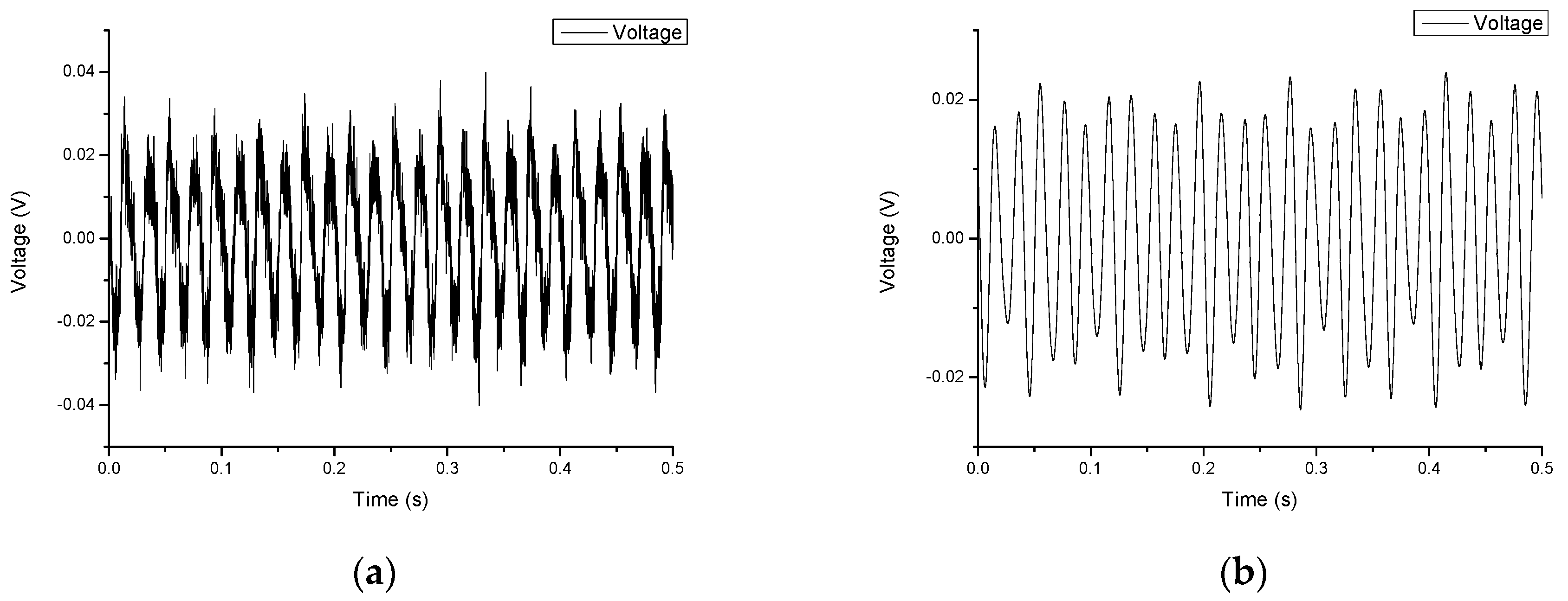
The noise pressure in a short period when a two-blade propeller is running at 1500 RPM is shown in Figure 6a. Note that the sound pressure signals have been transformed into voltage signals by the microphones.
According to the Mallat wavelet transform, the maximum passing frequency of the approximation signal in the next layer is half of the approximation signal in the upper layer. Low-frequency signals without high-order harmonics of BPF can be obtained by only eight-layer decomposition and reconstruction of the wavelet for the collected noise data when the propeller is running at 1500 RPM. In this paper, the noise data is decomposed into eight layers by the dB 30 wavelet cluster. The dB 30 wavelet base is equivalent to a specific set of low-pass filters H and high-pass filters G in Figure 5. The extracted noise signal after eight-layer decomposition and reconstruction is shown in Figure 6b.
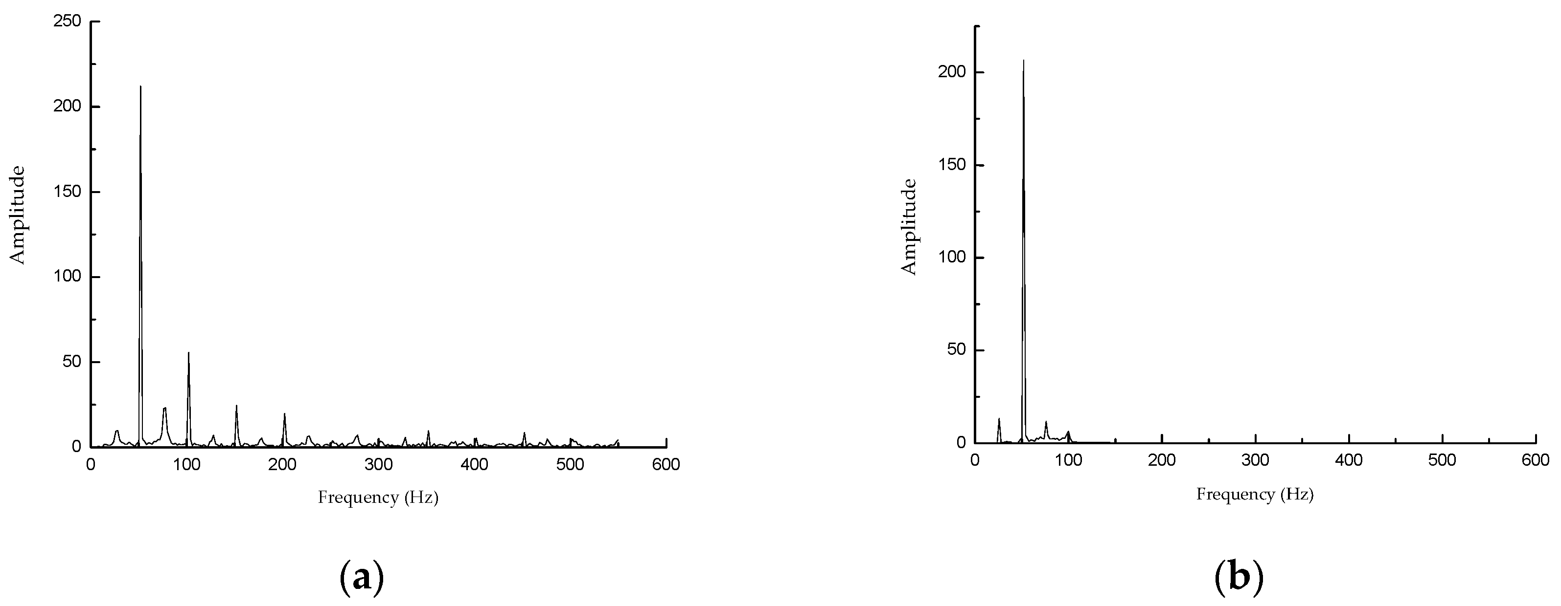
Fourier transform is performed on the original signal and the wavelet reconstructed signal in Figure 6, respectively, to obtain the spectrum as shown in Figure 7.
It can be seen from Figure 7a that the spectrum consists of a series of discrete frequencies where the frequency of the largest peak is 50 Hz (propeller BPF signal), and the amplitude of the BPF signal is much larger than other signals, which indicates that the noise energy of the propeller is mostly concentrated on the low frequency signal containing the BPF signal. Thus, the fluctuation of the low frequency signal can directly reflect the fluctuation of the propeller noise. The spectrum of the wavelet reconstructed signal removes the high-order harmonic signal of BPF and a large number of other high-frequency interference signals. Only the BPF signal and a small amount of other low-frequency, low-amplitude signals remain. The spectrum amplitudes at BPF before and after the wavelet transform are very close, thus the reconstructed signal is approximately the BPF signal. However, the high-order harmonic signal and part of the low-frequency signal of the BPF in Figure 7a also have non-negligible amplitude, and high-order harmonic signal of the BPF are greatly affected by the disturbance. For example, if the rotational speed of the propeller fluctuates about 60 RPM (1 Hz), the 4th BPF harmonic frequency will fluctuate about 8 Hz, and the amplitude change has no regular pattern. In this paper, the wavelet transform is used to extract the stable signal from the propeller noise. The goal is that the extracted signal can reflect the fluctuation of the propeller noise data and avoid using the fluctuating data for the propeller signature model identification. The ratio of the energy of the BPF high-order harmonic over the entire signal is low. The fluctuation is also large and the regularity is weak. It is indicated that BPF higher-order harmonics are not suitable for describing propeller noise data fluctuations. When the extracted signal contains both the BPF signal and the BPF high-order harmonic signal, the fluctuation may be very complex, which lowers the accuracy of the identification.
The wavelet extraction algorithm proposed in this section obtains the low frequency signal containing the BPF signal directly from the propeller noise, which effectively eliminates the interference of the BPF high-order harmonic signal and high-frequency noise. Comparing the low frequency components between Figure 7a,b, two peaks occur at 25 Hz and 75 Hz. The peak at 75 Hz is somehow filtered out in Figure 7b with respect to Figure 7a. This shows that the wavelet filter also has a significant filtering effect on the low-frequency interference component of the propeller noise, thereby maximally retaining the BPF signal component.
Ideally, the low frequency signal used to describe noise fluctuations retains only the BPF signal, but in Figure 7b, there is a small amount of low frequency signal at 25 Hz which is the rotational frequency at 1500 RPM. The amplitude of the 25 Hz signal in Figure 7 is less than 1/20 of the BPF signal. This means that most of the data fluctuations are not caused by the 25 Hz signal. According to Blunt [20], several flight tests of synchrophasing control under different flight conditions (flight velocity and height) were conducted and the rotational frequency and its harmonic are found to have little impact on the noise level. Thus, the small peak at 25 Hz in Figure 7b is believed to have no influence on the accuracy of the model and is retained in the reconstructed signal.
4.2. Sinusoidal Noise Signal Selection
Because the low frequency signal of the propeller is similar to the ideal sinusoidal signal, the ideal sinusoidal signal can be used to measure the propeller noise fluctuations. The propeller sinusoidal signal can be extracted from the actual propeller low frequency signal according to the least squares method. The Root Mean Squares Error (RMSE) between the actual propeller low-frequency signal and the fitting of the propeller BPF signal can be used as the evaluation criteria of the propeller noise fluctuation magnitude. The BPF signal can be expressed as
where A, ω, β0, and D0 are the amplitude, frequency, initial phase, and deviation error of the propeller BPF signal respectively. Four parameters need to be determined by the actual measurement data. The propeller speed generally fluctuates very little. In this paper, the rotational speed is set to be 1500 RPM and the fluctuation is only ±1 RPM (±0.03 Hz). The frequency error is only 0.67%, thus the error is negligible; in other words, the parameter ω is fixed once the rotational speed is fixed. If ω is known, the solution to the other parameters in Equation (6) is called the three-parameter method (TPM). If ω is unknown, the solution to all the parameters in Equation (6) is called the four-parameter method (FPM). Generally, the calculation of TPM is less than that of FPM [36]. The accuracy of the parameter ω would not be affected by using TPM due to the fact that the actual fluctuation of propeller rotation speed is small. Equation (6) can be expanded as
where ω is already known as the frequency. TPM is adopted to choose the appropriate parameters to fit the sinusoidal signal by making the sum of the squares of the residuals minimum. The residuals E is defined as
where are the least squares fit values of A, B, and D in Equation (7), respectively, n is the number of fitted data points, yi represents the original signal value. To solve , the following matrix is constructed
Then, E is rewritten as
When the residuals is the smallest, the least squares solution of the available x is
and the RMSE is
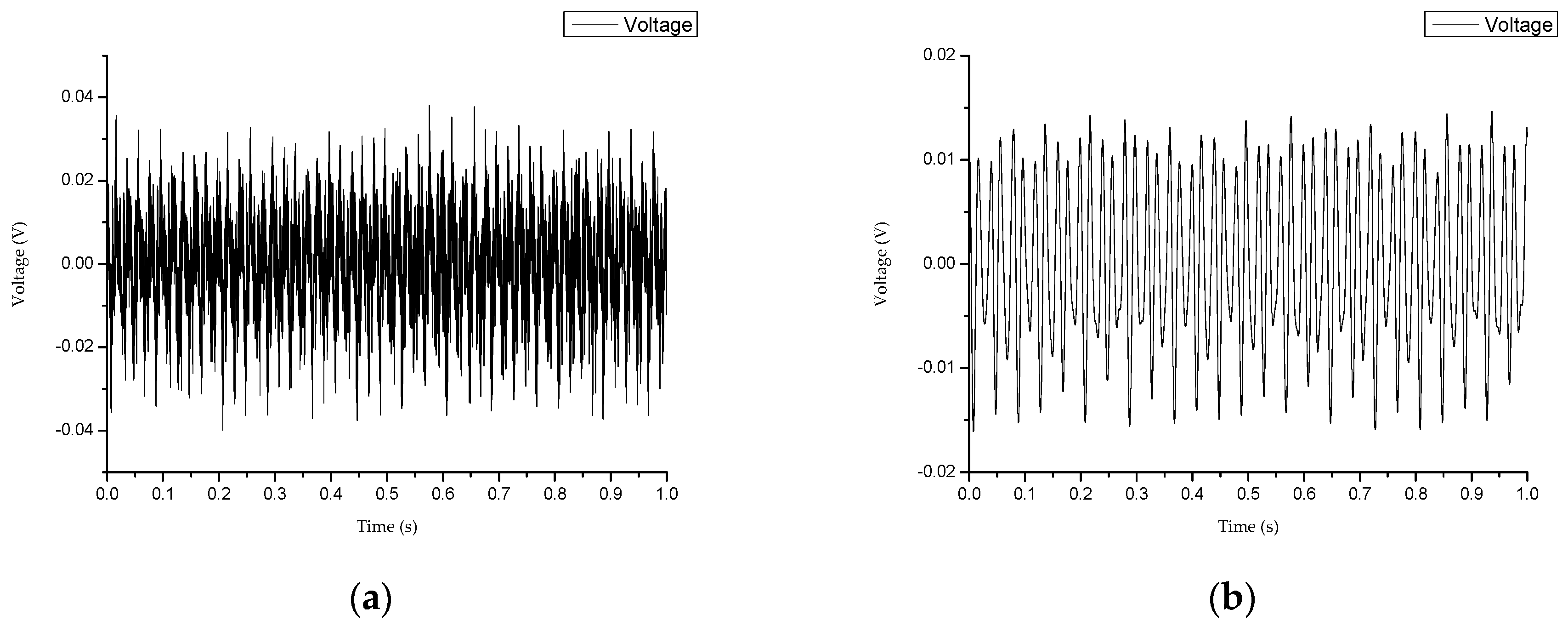
The following takes the phase angle combination data as an example to introduce the selection process of the minimum fluctuation data segment. The noise data is collected under the phase angle pair , and the noise data in the 0–1 s period is shown in Figure 8.
The reconstructed signal depicted in Figure 8b is filtered and restored by the wavelet transform mentioned in Section 4.1. According to the sinusoidal noise signal selection method introduced in this section, the RMSE of the segment data is 0.3915 dB. Note that the unit of the RMSE in this paper is dB according to the Equations (7)–(12). The RMSE of the data for each time period (starting at integral second) in 10 s is calculated as the same process of 0–1 s. The residuals are listed in Table 2. It can be seen that the data segment of 6–7 s has the smallest RMSE, which indicates that the noise fluctuation is the least during this period. Therefore, the data of this time period should replace the 4–5 s noise data used in Section 3 for higher identification accuracy.
4.3. Noise Model Identification and Accuracy Comparison
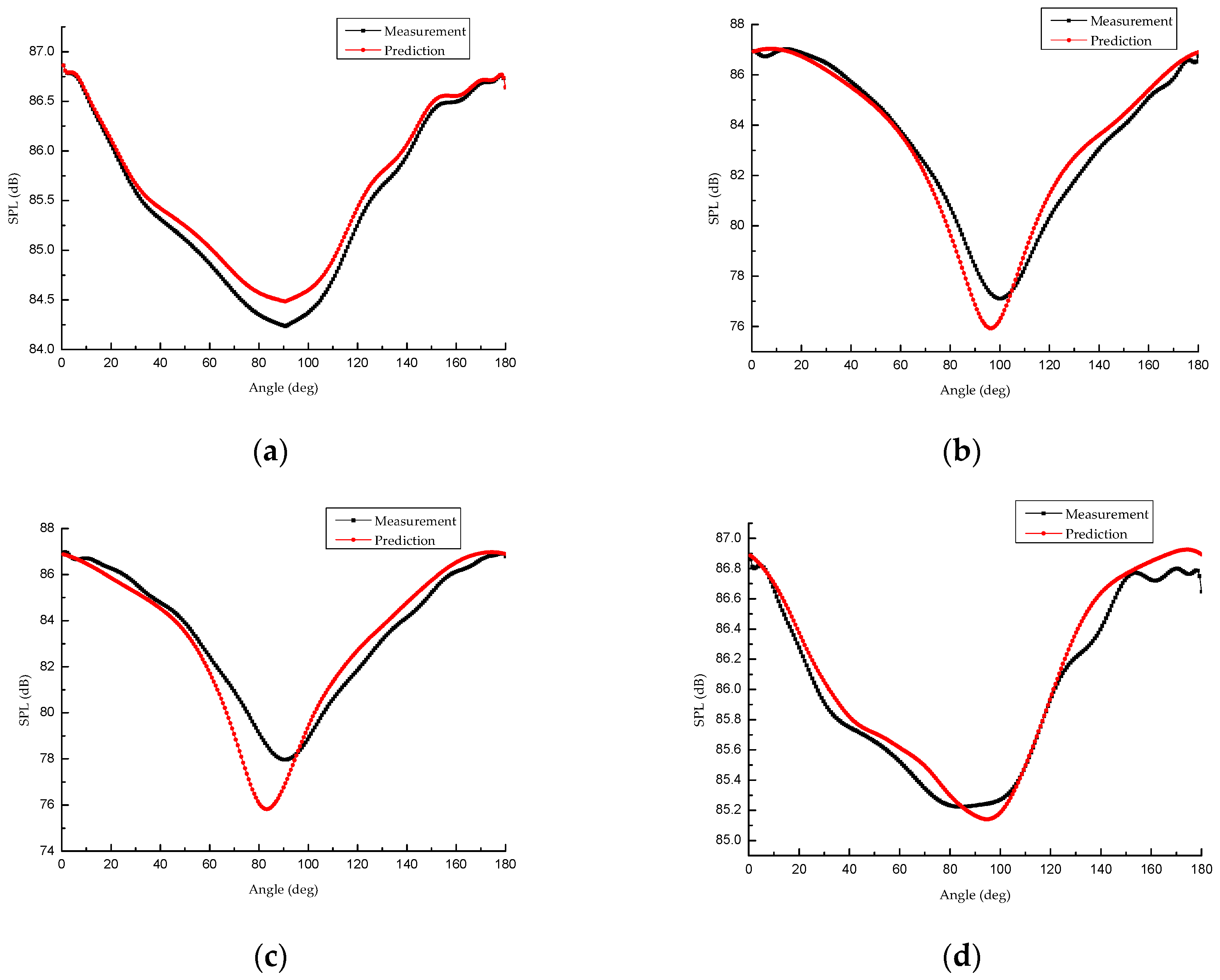
For other phase angle pairs, the noise data of the 10 s duration are collected. According to the process described in the previous section, the minimum fluctuation time periods are respectively calculated. Then, the propeller signature model is reidentified by noise data of the minimum fluctuation. The results are illustrated in Figure 9. The black line in the figure represents the actual noise level at the observer location and the red line represents the noise predicted by the identified propeller signature model.
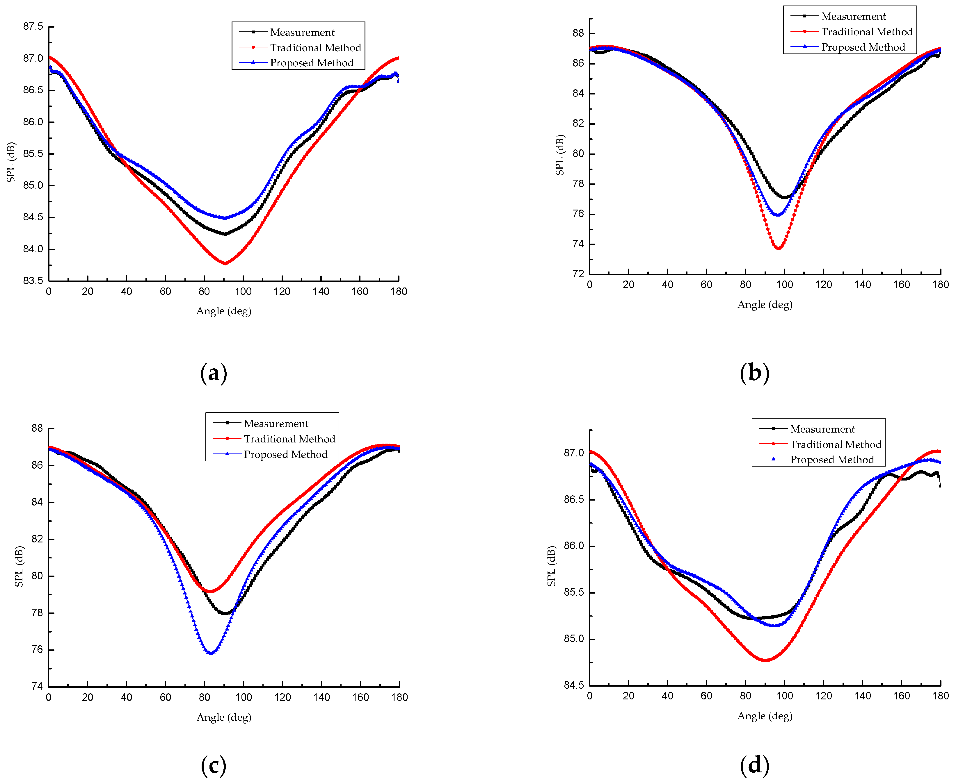
As shown in Figure 3 and Figure 9, the optimal phase angles predicted by the two methods are both close to the true optimal phase angle, and the errors are within 10 degrees. Better agreement is achieved at the No.1 microphone location between the prediction and the real noise by using the minimum data fluctuation selection method. This conclusion is still true for the other locations. Table 3 illustrates the absolute errors of the optimal phase angles and corresponding SPL predicted by two methods versus the real values. Comparisons of the complete curves predicted by traditional and proposed algorithm are shown in Figure 10. The black line in the figure represents the actual noise level at the observer location, the red line represents the noise predicted by the traditional method, and the blue line is the prediction of the minimum data fluctuation selection method.
The curves of the proposed method are closer to those of the real noise data than those of the traditional method. This demonstrates that the propeller signature model obtained by the proposed algorithm has higher accuracy than the model obtained by directly selecting the data of the arbitrary time. Noise data of other time periods (such as the 6–7 s etc.) may be used for model identification, and the effect may be better than the case of 4–5 s. However, this is not universal, and certain data segments, e.g., 6–7 s, cannot guarantee good modeling accuracy at all times. However, using the minimum data fluctuation selection method ensures that the data used for model identification has the least fluctuation and the accuracy of the noise model is thus guaranteed. As mentioned in Section 2, synchrophasing control is applicable in other scenarios. According to the data selection process, neither the number of the propellers nor the number of the blades per propeller is needed; this method can also be promoted to the other setup where the number of the blades per propeller is different. However, an experiment needs to be established to validate this and will be a future task.
5. Conclusions
In this paper, a propeller synchrophasing control experimental platform with a cylindrical scaled fuselage is built to explore the noise reduction inside the cabin. Propeller synchrophasing control can significantly attenuate the sound pressure level at the noise measurement locations with maximum reduction up to 19.5 dB. Wavelet filtering is adopted to extract the BPF signal of propeller noise; afterwards, three-parameter sine fitting algorithm is applied to select the data segment with the least fluctuation. Using the data segment with the least fluctuation for the propeller signature model identification can avoid modeling error caused by the transient disturbance of the sound pressure. Compared with the traditional fixed data segment identification model, the model identified by the proposed method has higher precision. However, the proposed method is not always better in all measurement locations, as Figure 10c shows a negative result. The better performance of the proposed method shown in Figure 10a,b,d may depend upon the given case, thus more experiments of different working conditions should be conducted in the future. Besides, the reflection of the wooden structure of the platform may account for the difference between the prediction and the real SPL and this could be a topic for future research.
Author Contributions
Conceptualization, L.S.; Methodology, L.S. and Y.C.; Software, Y.C.; Validation, L.S. and Y.C.; Formal Analysis, L.S.; Investigation, L.S. and Y.C.; Resources, L.S. and Y.C.; Data Curation, Y.C.; Writing—Original Draft Preparation, L.S.; Writing—Review and Editing, L.S.; Visualization, Y.C.; Supervision, X.H.; Project Administration, X.H.; Funding Acquisition, X.H.
Funding
This research was funded by National Natural Science Foundation of China, grant number 51576097 and Funding of Jiangsu Innovation program for Graduate Education, grant number KYLX15_0253 and the Fundamental Research Funds for the Central Universities.
Acknowledgments
The authors would like to thank members of the Nanjing University of Aeronautics and Astronautics and Jiangsu Province Key Laboratory of Aerospace Power System for their significant comments on this work.
Conflicts of Interest
The authors declare no conflict of interest.
Abbreviations
The following abbreviations have been employed in this work:
| BPF | Blade Passing Frequency |
| SPL | Sound Pressure Level |
| RPM | Revolutions per Minute |
| TPM | Three-Parameter Method |
| FPM | Four-Parameter Method |
| RMSE | Root Mean Square Error |
| Am | Resultant Noise Amplitude |
Appendix A

Table A1.
Different orders of the BPF harmonics affecting the accuracy of the model at the location of the No.2 microphone.
Table A1.
Different orders of the BPF harmonics affecting the accuracy of the model at the location of the No.2 microphone.
| Harmonic Order | 1 | 2 | 3 | 4 | 5 |
| Optimal phase angle | 20.3° | 18.3° | 15.4° | 11.6° | 8.4° |
| Corresponding SPL | 4.1 dB | 3.9 dB | 5.0 dB | 3.9 dB | 4.1 dB |
| Harmonic Order | 6 | 7 | 8 | 9 | 10 |
| Optimal phase angle | 6.2° | 4.1° | 4.0° | 3.7° | 3.7° |
| Corresponding SPL | 3.8 dB | 3.8 dB | 3.6 dB | 3.4 dB | 3.4 dB |
The data of the real noise is obtained by the traditional method at the location of the No.2 microphone. The optimal angle is 100.4° and the corresponding SPL is 77 dB. The data in the table above represent the absolute error between the prediction made by the different BPF harmonic orders and the real values. As the order increases, the optimal phase angle is closer to the real value, while the corresponding SPL is somehow smooth. When the harmonic order is higher than six, the error of the optimal phase angle is decreasing slower than the first six orders. This means that the first six orders are essential to identify the model and this is also demonstrated in the literature [6]. Note that the optimal phase angle predicted by the first ten harmonic orders is closer to the real one than that of the first six orders, which indicates that the higher the orders, the more accurate the result. Thus, both methods using the first ten orders of the BPF harmonic in this paper are reasonable and accurate.
References
- Magliozzi, B.; Hanson, D.B.; Amiet, R.K. Propeller and propfan noise. Aeroacoustics Flight Veh. Theory Pract. 1991, 1, 1–64. [Google Scholar]
- Li, X.; Sun, X.; Hu, Z.; Zhou, S. A new improved mean face method of subsonic propeller noise prediction. Chin. J. Aeronaut 1994, 15, 769–773. [Google Scholar] [CrossRef]
- Mathur, G.P. Active control of aircraft cabin noise. J. Acoust. Soc. Am. 1995, 5, 3267. [Google Scholar] [CrossRef]
- Hansen, C.; Snyder, S.; Qiu, X. Active Control of Noise and Vibration; CRC Press: Cleveland, OH, USA, 2012. [Google Scholar]
- Blunt, D.M.; Rebbechi, B. Propeller synchrophase angle optimisation study. In Proceedings of the 13th AIAA/CEAS Aeroacoustics Conference (28th AIAA Aeroacoustics Conference), Rome, Italy, 21–23 May 2007; pp. 3584–3594. [Google Scholar] [CrossRef]
- Huang, X.; Sheng, L.; Wang, Y. Propeller synchrophase angle optimization of turboprop-driven aircraft—An experimental investigation. J. Eng. Gas Turbines Power 2014, 136, 112606:1–112606:9. [Google Scholar] [CrossRef]
- Sheng, L.; Camino, F.M.; Huang, X. Synchrophasing control based on tuned ADRC with applications in turboprop driven aircraft. Control Eng. Appl. Inf. 2018, 20, 100–108. [Google Scholar]
- Murray, H.H.; Devenport, W.J.; Alexander, W.N.; Glegg, S.A.L.; Wisda, D. Aeroacoustics of a rotor ingesting a planar boundary layer at high thrust. J. Fluid Mech. 2018, 850, 212–245. [Google Scholar] [CrossRef]
- Atassi, H.; Logue, M. Fan broadband noise in anisotropic turbulence. In Proceedings of the 15th AIAA/CEAS Aeroacoustics Conference (30th AIAA Aeroacoustics Conference), Miami, FL, USA, 11–13 May 2009. [Google Scholar] [CrossRef]
- Murphy, J.P.; Macmanus, D.G. Inlet ground vortex aerodynamics under headwind conditions. Aerosp. Sci. Technol. 2011, 15, 207–215. [Google Scholar] [CrossRef]
- Stephens, D.; Morris, C. Sound generation by a rotor interacting with a casing turbulent boundary layer. AIAA J. 2009, 47, 2698–2708. [Google Scholar] [CrossRef]
- Marito, J.; Sipilä, T.; Sanchez-Caja, A.; Saisto, I. Evaluation of the propeller hull vortex using a RANS solver. In Proceedings of the 2nd International Symposium on Marine Propulsors, Hamburg, Germany, 15–17 June 2011. [Google Scholar]
- Glegg, S.A.L.; Buono, A.; Grant, J. Sound radiation from a rotor partially immersed in a turbulent boundary layer. In Proceedings of the 21st AIAA/CEAS Aeroacoustics Meeting, Dallas, TX, USA, 22–26 June 2015; pp. 2015–2361. [Google Scholar] [CrossRef]
- Magliozzi, B. Synchrophasing for cabin noise reduction of propeller-driven airplanes. In Proceedings of the 8th Aeroacoustics Conference, Atlanta, GA, USA, 11–13 April 1983; pp. 717–725. [Google Scholar] [CrossRef]
- Blunt, D.M.; Rebbechi, B. An investigation into active synchrophasing for cabin noise and vibration reduction in propeller aircraft. In Proceedings of the 6th International Symposium on Active Noise and Vibration Control, ACTIVE 2006, Institute of Noise Control Engineering, Adelaide, Australia, 18–20 September 2006. [Google Scholar]
- Blunt, D.M. Altitude and airspeed effects on the optimum synchrophase angles for a four-engine propeller aircraft. J. Sound Vib. 2014, 333, 3732–3742. [Google Scholar] [CrossRef]
- Johnston, J.F.; Donham, R.E.; Guinn, W.A. Propeller signatures and their use. J. Aircr. 1981, 18, 934–942. [Google Scholar] [CrossRef]
- Huang, X.; Wang, Y.; Sheng, L. Synchrophasing control in a multi-propeller driven aircraft. In Proceedings of the 2015 American Control Conference, Chicago, IL, USA, 1–3 July 2015; pp. 1836–1841. [Google Scholar] [CrossRef]
- Wang, Y.; Huang, X.; Zhang, T. An improved acoustic model identifying method in propeller synchrophasing control. Chin. J. Appl. Mech. 2014, 31, 933–938. [Google Scholar] [CrossRef]
- Kamiński, M. Homogenization-based finite element analysis of unidirectional composites by classical and multiresolutional techniques. Comput. Method Appl. Mech. 2005, 194, 2147–2173. [Google Scholar] [CrossRef]
- Belytschko, T.; Hughes, T.J.R. Computational Methods for Transient Analysis; North-Holland: Amsterdam, The Netherlands, 1983. [Google Scholar]
- Zienkiewicz, O.C.; Taylor, R.L.; Fox, D. The Finite Element Method: Solid Mechanics; Butterworth-Heinemann: Boston, MA, USA, 2000. [Google Scholar]
- Bacry, E.; Mallat, S.G.; Papanicolaou, G. A wavelet based space-time adaptive numerical method for partial differential equations. ESAIM Math. Model. Numer. 1992, 26, 793–834. [Google Scholar] [CrossRef] [Green Version]
- Gilbert, A.C. A comparison of multiresolution and classical one-dimensional homogenization schemes. Appl. Comput. Harmon. Anal. 1998, 5, 1–35. [Google Scholar] [CrossRef]
- Christon, M.A.; Roach, D.W. The numerical performance of wavelets for PDEs: the multi-scale finite element. Comput. Mech. 2000, 25, 230–244. [Google Scholar] [CrossRef] [Green Version]
- Al-Aghbari, M.; Scarpa, F.; Staszewski, W.J. On the orthogonal wavelet transform for model reduction/synthesis of structures. J. Sound Vib. 2002, 254, 805–817. [Google Scholar] [CrossRef]
- Jeong, H.; Jang, Y.S. Wavelet analysis of plate wave propagation in composite laminates. Compos. Struct. 2000, 49, 443–450. [Google Scholar] [CrossRef]
- Yam, L.H.; Yan, Y.J.; Jiang, J.S. Vibration-based damage detection for composite structures using wavelet transform and neural network identification. Compos. Struct. 2003, 60, 403–412. [Google Scholar] [CrossRef]
- Sung, D.U.; Kim, C.G.; Hong, C.S. Monitoring of impact damages in composite laminates using wavelet transform. Compos. Part B-Eng. 2002, 33, 35–43. [Google Scholar] [CrossRef]
- Frantziskonis, G. Wavelet-based analysis of multiscale phenomena: Application to material porosity and identification of dominant scales. Probab. Eng. Mech. 2002, 17, 349–357. [Google Scholar] [CrossRef]
- Blunt, D.M. Optimisation and Adaptive Control of Aircraft Propeller Synchrophase Angles. Ph.D. Dissertation, the University of Adelaide, Adelaide, Australia, 2012. [Google Scholar]
- Jones, J.D.; Fuller, C.R. Noise control characteristics of synchrophasing II-Experimental investigation. AIAA J. 1986, 24, 1271–1276. [Google Scholar] [CrossRef]
- Witte, R.A. Spectrum and Network Measurements; Scitech Publ: New York, NY, USA, 2014. [Google Scholar]
- Mallat, S.G. A theory for multiresolution signal decomposition: the wavelet representation. IEEE Trans. Pattern Anal. Mach. Intell. 1989, 11, 674–693. [Google Scholar] [CrossRef] [Green Version]
- Mallat, S.G. Multifrequency channel decompositions of images and wavelet models. IEEE Trans. Signal Process. 1989, 37, 2091–2110. [Google Scholar] [CrossRef]
- Liang, Z.; Meng, X. Review of Sine Wave Curve-Fit Methods. J. Test Meas. Technol. 2010, 24, 1–8. [Google Scholar] [CrossRef]
Figure 1.
Propeller signature schematic diagram: (a) phase angle pair of ; (b) phase angle pair of .
Figure 1.
Propeller signature schematic diagram: (a) phase angle pair of ; (b) phase angle pair of .


Figure 2.
Propeller synchrophasing control experimental platform: (a) Overall structure of the platform; (b) Cabin interior structure.
Figure 2.
Propeller synchrophasing control experimental platform: (a) Overall structure of the platform; (b) Cabin interior structure.


Figure 3.
Sound pressure level (SPL) over the angle range 0–180° at four microphone locations: (a) No.1 installation hole; (b) No.2 installation hole; (c) No.3 installation hole; (d) No.4 installation hole.
Figure 3.
Sound pressure level (SPL) over the angle range 0–180° at four microphone locations: (a) No.1 installation hole; (b) No.2 installation hole; (c) No.3 installation hole; (d) No.4 installation hole.

Figure 4.
SPL changes with .

Figure 5.
Wavelet transform: (a) decomposition algorithm; (b) reconstruction algorithm.

Figure 6.
Original and reconstructed signal of propeller noise: (a) Original signal; (b) reconstructed signal.
Figure 6.
Original and reconstructed signal of propeller noise: (a) Original signal; (b) reconstructed signal.

Figure 7.
Signal spectrum: (a) Propeller noise signal spectrum; (b) Reconstructing signal spectrum.

Figure 8.
0–1 s original and reconstructed signal: (a) original signal; (b) reconstructed signal.

Figure 9.
SPL over the angle range 0–180° at four microphone locations by the minimum data fluctuation selection method: (a) No.1 installation hole; (b) No.2 installation hole; (c) No.3 installation hole; (d) No.4 installation hole.
Figure 9.
SPL over the angle range 0–180° at four microphone locations by the minimum data fluctuation selection method: (a) No.1 installation hole; (b) No.2 installation hole; (c) No.3 installation hole; (d) No.4 installation hole.

Figure 10.
Comparisons of predictions versus the real noise data by the traditional and proposed algorithm: (a) No.1 installation hole; (b) No.2 installation hole; (c) No.3 installation hole; (d) No.4 installation hole.
Figure 10.
Comparisons of predictions versus the real noise data by the traditional and proposed algorithm: (a) No.1 installation hole; (b) No.2 installation hole; (c) No.3 installation hole; (d) No.4 installation hole.

Table 1.
Angle pairs selected for the identification.
| Angle pair No. Angle value | 1 | 2 |
| Angle pair No. Angle value | 3 | 4 |
| Angle pair No. Angle value | 5 | 6 |
| Angle pair No. Angle value | 7 | 8 |
Table 2.
RMSE of ten data segments.
| Time/s | 0–1 | 1–2 | 2–3 | 3–4 | 4–5 |
| RMSE | 0.3915 dB | 0.4154 dB | 0.4394 dB | 0.4681 dB | 0.3953 dB |
| Time/s | 5–6 | 6–7 | 7–8 | 8–9 | 9–10 |
| RMSE | 0.3869 dB | 0.3579 dB | 0.3836 dB | 0.3913 dB | 0.3904 dB |
Table 3.
Optimal phase angles and corresponding SPL predicted by two methods.
| Optimal phase angle | Mic No.1 | Mic No.2 | Mic No.3 | Mic No.4 |
| Traditional algorithm | 0.0° | 3.7° | 8.2° | 6.0° |
| Proposed algorithm | 0.0° | 3.7° | 7.4° | 10.4° |
| SPL at optimal phase angle | Mic No.1 | Mic No.2 | Mic No.3 | Mic No.4 |
| Traditional algorithm | 0.5 dB | 3.4 dB | 1.2 dB | 0.5 dB |
| Proposed algorithm | 0.3 dB | 1.2 dB | 2.1 dB | 0.1 dB |
© 2019 by the authors. Licensee MDPI, Basel, Switzerland. This article is an open access article distributed under the terms and conditions of the Creative Commons Attribution (CC BY) license (http://creativecommons.org/licenses/by/4.0/).
Share and Cite
MDPI and ACS Style
Sheng, L.; Huang, X.; Cao, Y. Propeller Synchrophasing Control with a Cylindrical Scaled Fuselage Based on an Improved Data Selection Algorithm. Energies 2019, 12, 2736. https://doi.org/10.3390/en12142736
AMA Style
Sheng L, Huang X, Cao Y. Propeller Synchrophasing Control with a Cylindrical Scaled Fuselage Based on an Improved Data Selection Algorithm. Energies. 2019; 12(14):2736. https://doi.org/10.3390/en12142736
Chicago/Turabian StyleSheng, Long, Xianghua Huang, and Yunfei Cao. 2019. "Propeller Synchrophasing Control with a Cylindrical Scaled Fuselage Based on an Improved Data Selection Algorithm" Energies 12, no. 14: 2736. https://doi.org/10.3390/en12142736
Note that from the first issue of 2016, this journal uses article numbers instead of page numbers. See further details here.