Lifecycle Energy Accounting of Three Small Offshore Oil Fields

Program in Systems Engineering, Walter Scott Jr. College of Engineering, Colorado State University, Fort Collins, CO 80523-1302, USA
*
Author to whom correspondence should be addressed.
Energies 2019, 12(14), 2731; https://doi.org/10.3390/en12142731
Submission received: 7 June 2019
/
Revised: 30 June 2019
/
Accepted: 15 July 2019
/
Published: 17 July 2019
Abstract
:Small oil fields are expected to play an increasingly prominent role in the delivery of global crude oil production. As such, the Energy Return on Investment (EROI) parameter for three small offshore fields are investigated following a well-documented methodology, which is comprised of a “bottom-up” estimate for lifting and drilling energy and a “top-down” estimate for construction energy. EROI is the useable energy output divided by the applied energy input, and in this research, subscripts for “lifting”, “drilling”, and “construction” are used to differentiate the types of input energies accounted for in the EROI ratio. The EROILifting time series data for all three fields exhibits a decreasing trend with values that range from more than 300 during early life to less than 50 during latter years. The EROILifting parameter appears to follow an exponentially decreasing trend, rather than a linear trend, which is aligned with an exponential decline of production. EROILifting is also found to be inversely proportional to the lifting costs, as calculated in USD/barrel of crude oil. Lifting costs are found to range from 0.5 dollars per barrel to 4.5 dollars per barrel. The impact of utilizing produced gas is clearly beneficial and can lead to a reduction of lifting costs by as much as 50% when dual fuel generators are employed, and more than 90% when gas driven generators are utilized. Drilling energy is found to decrease as the field ages, due to a reduction in drilling intensity after the initial production wells are drilled. The drilling energy as a percentage of the yearly energy applied is found to range from 3% to 8%. As such, the EROILifting+Drilling value for all three fields approaches EROILifting as the field life progresses and the drilling intensity decreases. The construction energy is found to range from 25% to 63% of the total applied energy over the life of the field.
1. Introduction
Giant oil fields have been described in a number of ways, but a generally accepted definition is a field which has a daily production rate that exceeds one hundred thousand barrels of oil per day or Ultimate Recoverable Reserves (URR) of greater than 500 million barrels of oil [1]. There are believed to be more than 500 giant fields in existence, which only constitute approximately 1% of the total number of oil fields but account for approximately 60% of global daily oil production [1]. The remaining 40% of global daily production is produced by smaller fields that tend to receive considerably less attention than the giant fields. It is widely believed that the contribution of smaller fields to global production will gradually increase over time [2]. This due to the fact that many of the existing giant fields are over 50 years old and are experiencing declining production. Another factor is the decline in discoveries of giant fields that are needed to replace the existing depleted giant fields [1]. As such, it is worthwhile to gain a better understanding of small oil fields in terms of their energetic characteristics.
Energy accounting is a valuable method used to understand the energetic characteristics of systems and to distinguish between different types of systems, such as between large scale and small scale oil and gas developments. Energy accounting can be used to gain insight into the value-added nature of an oil and gas development and supplement economic analysis [3,4,5]. It is readily apparent that nearly all of the economical drivers of oil and gas production operations are related to energy. For example, oil and gas costs are fundamentally underpinned by energy utilization, such as with regards to the energy used to drive drilling equipment, the energy used to power the devices that lift fluids from the reservoir to the surface, and the energy used to drive the surface processing equipment. There is also a significant amount of energy expended to construct and assemble surface facilities. Other forms of energy consumption in oil and gas operations are less apparent and more difficult to quantify, such as the energy expended to support logistical activities, or the energy consumed by the labor force, both in the field and in the business office. Three very important and quantifiable categories of oil field energy utilization are with respect to construction, drilling, and lifting.
The first law of thermodynamics states that energy is conserved, but if the purpose of the analysis is to better understand the energy efficiency of a process, then only the invested energies into the system and only the returned energies out of the system need to be considered. The returned energy out of the system is simply the chemical energy in the crude oil product, which is normally described by the heating value. The ratio of returned energy output to invested energy input, as described by Equation (1), is commonly referred to as the Energy Return on Investment (EROI), a parameter that has been applied to a wide number of energy-related industries. Concerning the oil and gas industry, there have been numerous EROI studies covering a wide range of boundaries, such as for global production, for country level production, and for specific fields [6,7,8,9,10,11,12,13,14,15,16,17,18,19,20,21].
The EROI parameter can be used to better understand the energetic effectiveness of oil and gas producing schemes and how it changes over time. A well-structured method is required to consistently analyze the EROI of an oil and gas extraction process, and fortunately a lot of progress has been made in this area. Firstly, a standardized method for defining the boundaries for the inputs and outputs was developed by Murphy et al. The boundaries and associated notations are described in Table 1 [13].
The horizontal EROI boundaries in Table 1 are indicated with numerical codes of 1, 2, and 3 and represent the main supply chain categories of: Extraction (1), Processing (2), or End-Use (3). The vertical boundaries are progressively cumulative such that the indicator “d” only includes direct energy and materials, while the indicator “standard” includes both direct and indirect energy and materials. After “standard”, the notation continues to cumulatively add energy categories as you move down the table, such as “lab”, “aux” and “env” which stand for the indirect labor energy consumption, auxiliary services energy consumption and environmental energy respectively. For example, the notation ‘EROI 2env” aggregates all five types of energy for the Processing supply chain category only. For crude oil, the extraction, initial processing, and transportation to the refinery is sometime referred to as the Well to Refinery (WTF) pathway [22].
It was suggested by Murphy et al. that EROI-standard could be a benchmarked parameter used to characterize the extraction process. The difficulty with the EROI-standard parameter is that it includes indirect materials and energy. Indirect energy may be the fuel used to run supporting equipment, such as ships, helicopters, and road transportation vehicles. Indirect materials are related to the energy used to form and build the secondary equipment. The practicality and usefulness to oilfield analysts of including these types of secondary energy contributions in the accounting exercise is questionable. Therefore, it is suggested that EROI-1d, which represents direct energy and materials for the extraction operation only, is a more practical benchmark with regards to oil and gas extraction operations. It is also suggested to consider subsets of EROI-1d to better understand the impact of construction, drilling, and lifting energies. The proposed approach is to progressively include more information in the EROI-1d parameter, as indicated in Table 2.
1.1. Lifting Energy
This research proposes the category “lifting energy”, which is the incremental energy used to produce one additional barrel of crude oil. The lifting energy include the energy required to produce reservoir fluids, the energy required to dispose associated water, and the energy required to stimulate the reservoir via secondary or tertiary recovery methods. The proposed EROI-1dLifting indicator is the ratio of the produced crude oil energy output to the lifting energy input. The minimum operational requirement of sustainable production is that the produced energy is greater than the lifting energy. This implies that the EROI-1dLifting must be greater than one. When the EROI-1dLifting value reaches unity, the operation is no longer energetically favorable, as there is no energy surplus being produced. This is the case regardless of any commercial factors, such as production commitments, the market price of oil, currency exchange rates, fiscal regimes, and tax rates. It is also equally applicable if the fuel source is derived from “free” produced fluids, such as from associated natural gas that has no path to market. In actuality, an EROI-1dLifting greater than one is required to offset energy intensive refining processes and end-use inefficiencies when liquid fuels are converted to useable forms of energy, such as shaft work and electricity. Therefore, a minimum EROI-1dLifting in the range of 3 to 5 is probably more realistic [23].
The proposed “lifting energy” category is considered to have the same constituents as lifting costs. Therefore, by understanding the lifting energetics, we can gain insight into the main influences to the lifting costs. Lifting energy, and therefore lifting costs, tend to increase as a field matures due to a number of reasons, two of which are increasing production of water and decreasing crude oil production. Empirical formulas have been developed to correlate lifting costs with percent recovery of the reservoir or with production rates [24], but these formulas are field specific due to the unique operational conditions of each field.
1.2. Drilling Energy
Drilling and completion of oil and gas wells is an energy intensive process, and consequently, the associated drilling costs are normally a significant portion of the overall development costs. Depending on the development, the drilling costs can be as much as 60% of the total Capital Expenditure [24]. In many fields, drilling is a continuous exercise that continues from year to year, as depleted wells are side-tracked, extended, or replaced. It is common to have annual drilling campaigns with multiple rigs servicing a single oil and gas development. The energy expended by a drilling rig can be estimated using a “bottom-up” approach, which takes into account the electrical loads applied in the various stages of drilling, such as drilling, tripping (running and pulling completions), standby, and transit. A very important parameter related to drilling energy, and costs, is the time it takes to drill and complete a well. This can range from a few days to a few months, depending on the well complexity. Therefore, it is necessary to understand the EROI-1dLifting+Drilling parameter due the fact that it can represent a substantial component of the continuous direct energy applied to an oil field.
1.3. Construction Energy
Finally, the construction of oil and gas facilities represents another energy intensive activity. Surface facilities for oil and gas operations are designed for the specific circumstances of the field with respect to the operating environment, fluid properties, and related processing requirements. Offshore fields typically require large steel structures to support the wellheads and processing equipment. Onshore facilities are normally delivered at a much lower cost than offshore facilities in terms of production capacity costs, which are reported in U.S. dollars per barrel per day (USD/BPD), but it depends on the unique qualities of the development. The method used to calculate construction energy can be either “top-down” or “bottom-up”. The bottom-up method, which is often used for the lifting and drilling categories, involves collecting detailed energy utilization data at the equipment level. With regards to construction, this type of information would need to cover a wide range of activities and is not readily available to oil and gas companies. Therefore, a top-down approach is more practical to use in most circumstances. The top-down method is to convert monetary expenditure to energy using published energy intensity values. For example, input/output tables have been developed covering a number of industries and commodities. These tables indicate the energy required for specific products, such as steel in MJ/ton, or can be developed for more generic industrial processes, such as with respect to heavy industry [3,8]. A figure that has been used in previous energy accounting work for oil and gas facilities is 14.5 MJ per dollar (2005 basis) [13]. Therefore, the EROI-1dLifting+Drilling+Construction is a relevant parameter that includes an aggregation of the most significant forms of direct energy applied to an oil extraction process, and is aligned with the original intention of the EROI-1d category, as defined by Murphy et al. [13].
1.4. Lifting Costs
The cost per barrel parameter has long been used as an economic decision tool in the oil and gas industry [25]. The term “lifting cost” is commonly used in the oil and gas industry to describe the incremental costs of producing one additional barrel of crude oil. The lifting cost is an important parameter affecting oil field economics and is normally reported in US dollars per barrel produced (USD/BBL). Lifting cost has been found to be a function of the following variables [26]:
- Gross rate;
- Oil rate;
- Gas rate;
- Injection water rate;
- Oil wells count;
- Gas wells count;
- Injection wells count.
It is notable that the lifting cost is more than the cost of raising reservoir fluids to the surface with artificial lift technologies, such as sucker rod pumps and electrical submersible pumps, as it also includes the costs of initial processing and injection, or disposal, of associated water or gas to comply with environmental requirements or to stimulate the reservoir. Initial processing includes separation of water and gas from the crude, stabilization of the crude to meet vapor pressure specifications for storage, treatment of water to remove oil, and treatment of the gas to be used as fuel. The variables listed above do not differentiate between water injection and disposal, but an important distinction is needed. In many parts of the world, associated water produced in the oil extraction process must be safely disposed of in subterranean reservoirs, rather than discharged to the sea or to evaporation pits, for example. The intention is to dispose the water in an environmentally acceptable way only, not to influence or stimulate the hydrocarbon bearing reservoir. For water disposal the preference is to pump the water into low pressure reservoirs to minimize the energy used by the disposal pumps and related costs. Primary recovery is defined by the exclusion of reservoir stimulation methods [27].
Conversely, water injection is a form of secondary recovery which is used to stimulate the hydrocarbon reservoir to maintain pressure or to sweep the hydrocarbons into extraction zones, a practice which is known as water-flooding [28,29]. The source of water can be treated with associated water, external seawater, or fresh water. Pressure maintenance and water-flooding usually entail the injection of water directly into the hydrocarbon reservoir at very specific locations, which is usually much deeper and at a higher pressure than disposal reservoirs. Therefore, water injection requires significantly more energy than water disposal, which implies higher lifting costs. There are many other types of energy intensive secondary recovery methods, such as pressure maintenance via gas injection, and reservoir sweeping mechanisms, such as gas flooding. All of these methods have an impact on the lifting cost.
Tertiary recovery methods are often labeled as “Enhanced Oil Recovery” (EOR), and entail more recent technologies, such as alternating water and gas injection, polymer flooding, and thermal recovery methods, such as steam injection [30,31,32,33]. Heavy oils with low viscosities often require reservoir stimulation via thermal methods, such as steam flooding, cyclic steam injection, informally known as “huff and puff” in the industry, or by the steam assisted gravity drainage (SAGD) method [34]. There has been extensive research into the economics, and hence lifting costs, of steam injection, which is characterized by an exceptionally high energy demand [35,36,37,38].
1.5. Internal vs. External Energy Sources
An additional dimension related to the source of direct energy used for EROI-Lifting was derived to differentiate between external and internal energy sources. Net Energy Return (NER) includes both internal and external energy investments, while External Energy Return (EER) only includes external energy investments such as imported fuel gas, liquid fuels such as diesel, and electricity imported from an external grid [17]. NER and EER ratios are described by Equations (2) and (3).
Therefore, to take into account the internal/external nature of the fuels used in lifting, the notation of NER and EER are appended to the front of the referenced nomenclature where applicable, such as:
- NER-EROI-1dLifting
- EER-EROI-1dLifting
- EER-EROI-1dLifting+Drilling
- EER-EROI-1dLifting+Drilling+Construction
NER (which includes both internal and external energy) is only applied to lifting, since internal energy is rarely used for drilling or construction activities.
1.6. Previous Work on Field-Specific EROI Derivations
There has been a considerable effort to develop field specific EROI calculation models and tools, such as the Oil Producing Greenhouse Emissions Estimator (OPGEE), which is a tool used to estimate field specific EROIs using a combined bottom-up and top-down approach [39]. The tool also employs smart defaults to assist with the EROI calculation when information is incomplete.
Consistently, field specific EROIs have been shown to decline over time as production declines and the energy intensity of the operation increases [14,19]. Brandt et al. used the OPGEE tool to calculate the time series EROIs of several giant oilfields over several decades. In this study, all fields experienced a significant decrease in EROI over time due to a combination of factors, including declining production rate, implementation of more rigorous recovery methods, and the application of more stringent environmental measures to dispose of unwanted byproducts [19].
There has been very little published work on developing EROIs for small fields, which as mentioned above are now emerging in terms of their importance. Small fields have a number of challenging characteristics, as opposed to large fields, such as shorter field lives and an inability to capitalize on economies of scale. Therefore, this research endeavors to illuminate the energetic behavior of three small offshore oil fields.
1.7. Summary of EROI Literature Influencing This Research
The following table presents some of the previous EROI research that influenced this research. The data presented is a high level summary. The methods used by the authors varied, but generally can be classified into two types; top-down and hybrid. The top down method entails converting published production rates and cost-to-energy equivalents. No attempt is made to estimate fuel consumption, for example, or to convert equipment and facilities information into energy equivalents. The hybrid approach supplements cost data with detailed engineering estimates for energy consumption. The boundaries the studies are not all readily apparent, but generally included extraction only, which is comprised of lifting, drilling, and construction activities.
1.8. Case Studies
As can be seen in Table 3, a great deal of research has been conducted on energy accounting and with derived EROIs covering a range of methods and boundaries. Only recently have individual fields been examined using engineering analysis with a variety of data sources and assumptions. There has been very little work published on developing EROIs for small fields, which as mentioned above are now emerging in terms of their importance. Small fields have a number of challenging characteristics, as opposed to large fields, such as shorter field lives, shorter time frames for decision making, and an inability to capitalize on economies of scale. Therefore, it is imperative for oil and gas operators to understand the energetic behavior and associated cost implications of small fields and be able to make informed, timely decisions.
This research attempts to illuminate the practical aspects of the energy accounting methodology by developing cases studies. A secondary goal is to describe the energetic and economic behavior of three small offshore fields. The selected three fields share some characteristics, such as the water depth, the lifting mechanism, the crude properties, the processing requirements, the processing capacities, and to some extent the requirement to dispose or inject water into subterranean reservoirs. The fields also have some important distinguishing aspects, which makes for interesting comparisons, with respect to recovery method and produced gas quality and quantity. These characteristics are described in Table 4.
What makes this research unique is the authors’ access to detailed field specific data. The ensuing analysis contains very few assumptions, as production rates and fuel consumption rates, including diesel fuel and natural gas, are based on actual field data. Furthermore, the researchers have access to original capital cost data for all three fields, as well as access to the detailed drilling program stretching back to the initial drilling campaign, and includes the actual drilling energies based on drilling equipment loads. Therefore, this research endeavors to illuminate the energetic behavior of three small offshore oil fields by analyzing actual detailed field level data.
2. Results and Discussion
Figure 1, Figure 2 and Figure 3 indicate the time series production rates of oil and water for three small offshore oil fields, along with the corresponding NER-EROI-1dLifting. It is clear that NER-EROI-1dLifting declines as crude production declines, or produced water increases in all three fields. The largest dataset was for Field 1 in terms of the time period covered, so the decreasing trend is more mature. It should be noted that Field 1 switched from high pressure water injection to low pressure disposal in 2001. Therefore, the decreasing NER-EROI-1dLifting was attenuated by this change in recovery strategy. The decision was based on the development team’s belief that natural aquifer drive was sufficient to maintain reservoir pressure and sweep the hydrocarbons into extraction zones. Regardless of the switch from was disposal to water injection, Field 1 exhibits decreasing crude and increasing water, and hence decreasing NER-EROI-1dLifting over its field life.
Fields 2 and 3, which employs high pressure water injection only, exhibit similar trends, although since they are both relatively young fields the data only covers the early phase of field life.
General trends for each field are shown in Table 5, indicating that all three fields experience decreasing NER-EROI-1dLifting under similar production trends.
It should be noted that all three fields have recently reached their current water handling capacity limit, a condition commonly referred to as “bottlenecked”. A debottlenecking campaign is underway to increase each field’s water handling capacity. The debottlenecking is needed to sustain crude oil production, but will result in an increase of energy consumption to handle and inject the additional water. Therefore, the EROI decreasing trends are expected to accelerate in the post-debottlenecking phase of operation for all three fields.
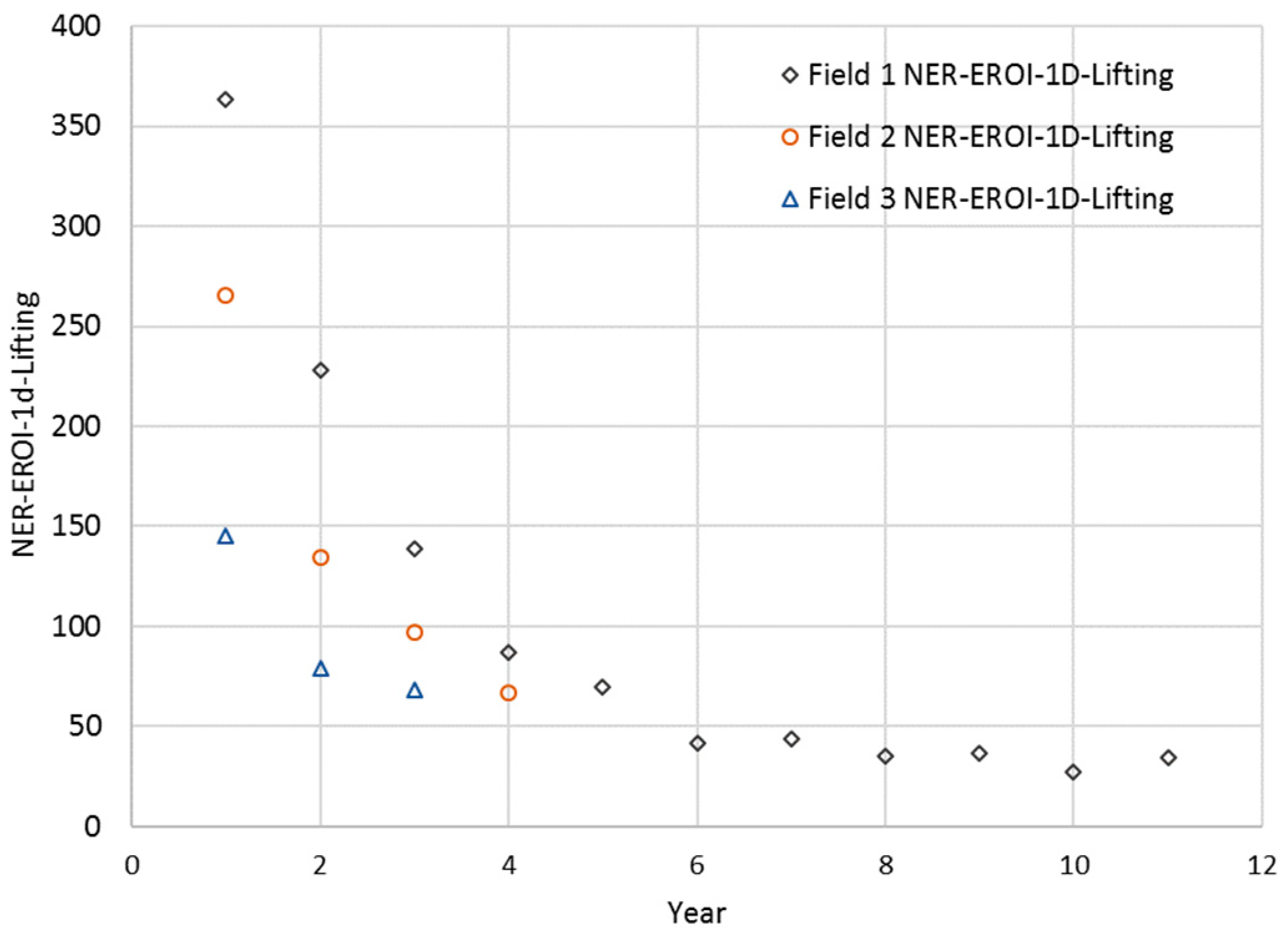
The NER-EROI-1dLifting time series trends for the three small fields included in this study are shown in Figure 4. The NER-EROI-1dLifting values all decline rapidly in the first years of production, followed by a slower decline in later years. The three fields exhibit a similar pattern of decline, which is caused by a combination of declining crude oil production and increasing water production.
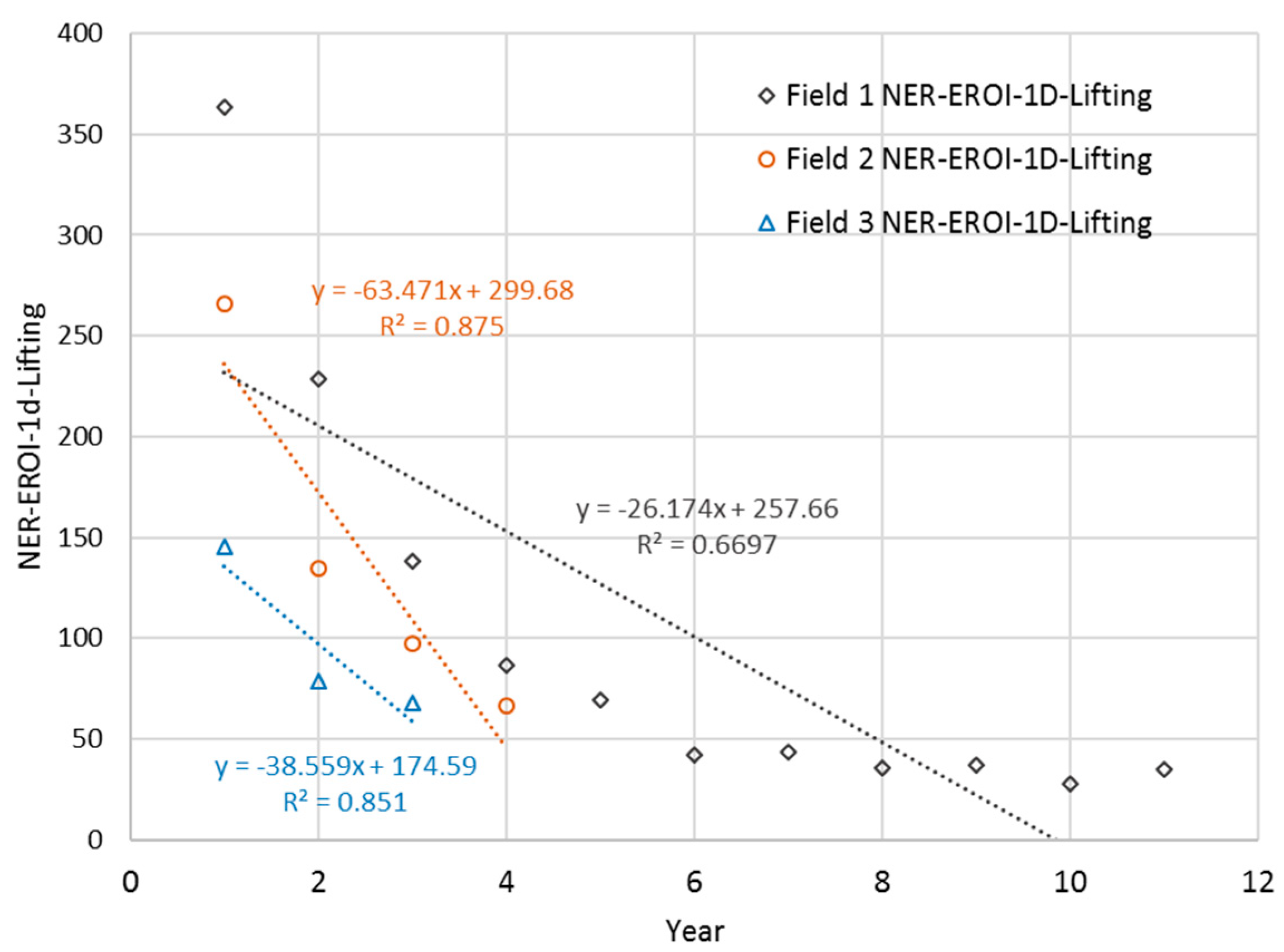
Linear and exponential regression analysis was applied to model the declining NER-EROI-1dLifting of the three fields. As can be seen in Figure 5, the fields exhibited differing slopes of decline. Fields 1 and 3 exhibited similar slopes, while Field 2 exhibited a steeper decline slope.
Exponential regression analysis was applied to the NER-EROI-1dLifting data and generally exhibited a better fit with regards to the R2 value, as indicated in Figure 6. Once again, Fields 1 and 3 exhibited similar exponential declines, as opposed to Field 2, which exhibited a much steeper decline. Crude oil production profiles are often modeled with exponential or hyperbolic decline functions [20]. Therefore, since the crude oil decline curve influences the EROI decline curve, it is hypothesized that an analogous EROI exponential decline approach may represent a reasonable model, and future work should revolve around developing mathematical decline models for NER-EROI-1dLifting.
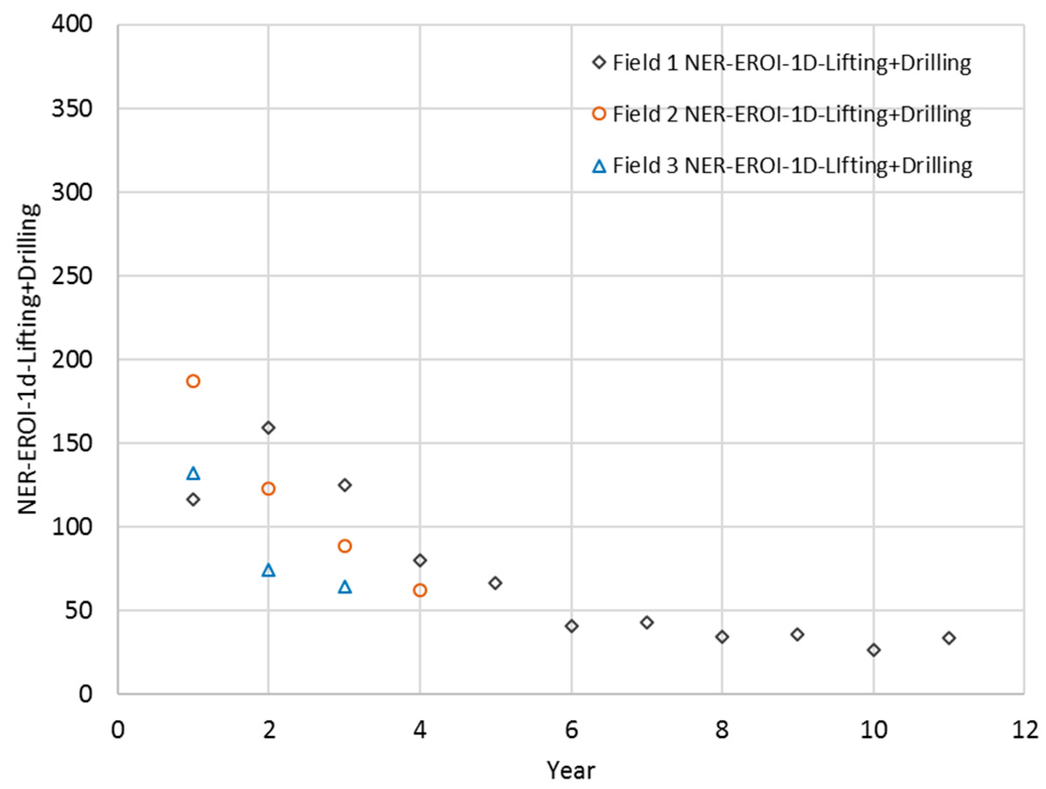
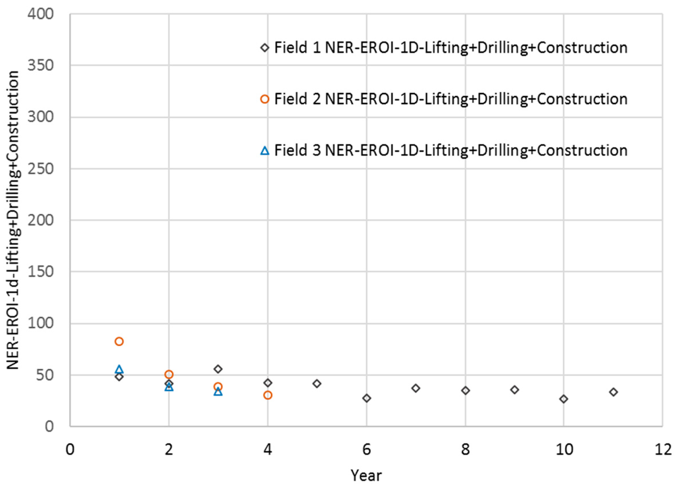
An interesting aspect of this work was the significance of drilling energy for all three fields. This can be understood by examining the differences between NER-EROI-1dLifting and NER-EROI-1dLifting+Drilling for each field, as exhibited in Figure 4 and Figure 7. Drilling energy calculations are shown in Appendix A, Figure A1. Generally speaking, the EROIs dropped from as much as 70% in early life to as little as 2% in later life. This indicates that the NER-EROI-1dLifting+Drilling approaches NER-EROI-1dLifting, as drilling activities are reduced from the initial intensive drilling phase of the field.
As shown in Figure 8, when drilling and construction energies are accounted for, the EROIs shift downward by up to 87% in early life from EROI-1dLifting, which only includes the lifting energy. Construction energy calculations are shown in Figure A1 and Figure A2. The construction energies are amortized over the first three years of production; therefore, the shift downward due to construction of facilities is realized only during the early years of production. The construction of offshore platforms that weigh between 1000 to 2000 tons is an energy-intensive process. Therefore, it is not surprising that there is a significant impact on EROIs when construction energies are included in the early years of production.
An energy balance time series, which does not amortize construction, was developed to better understand the following:
- Actual cumulative energy profile;
- The energy breakeven point for all the 3 fields;
- The annual proportion of energy-in from lifting, drilling, and construction;
- The overall (field-life) proportion of energy-in from lifting, drilling, and construction.
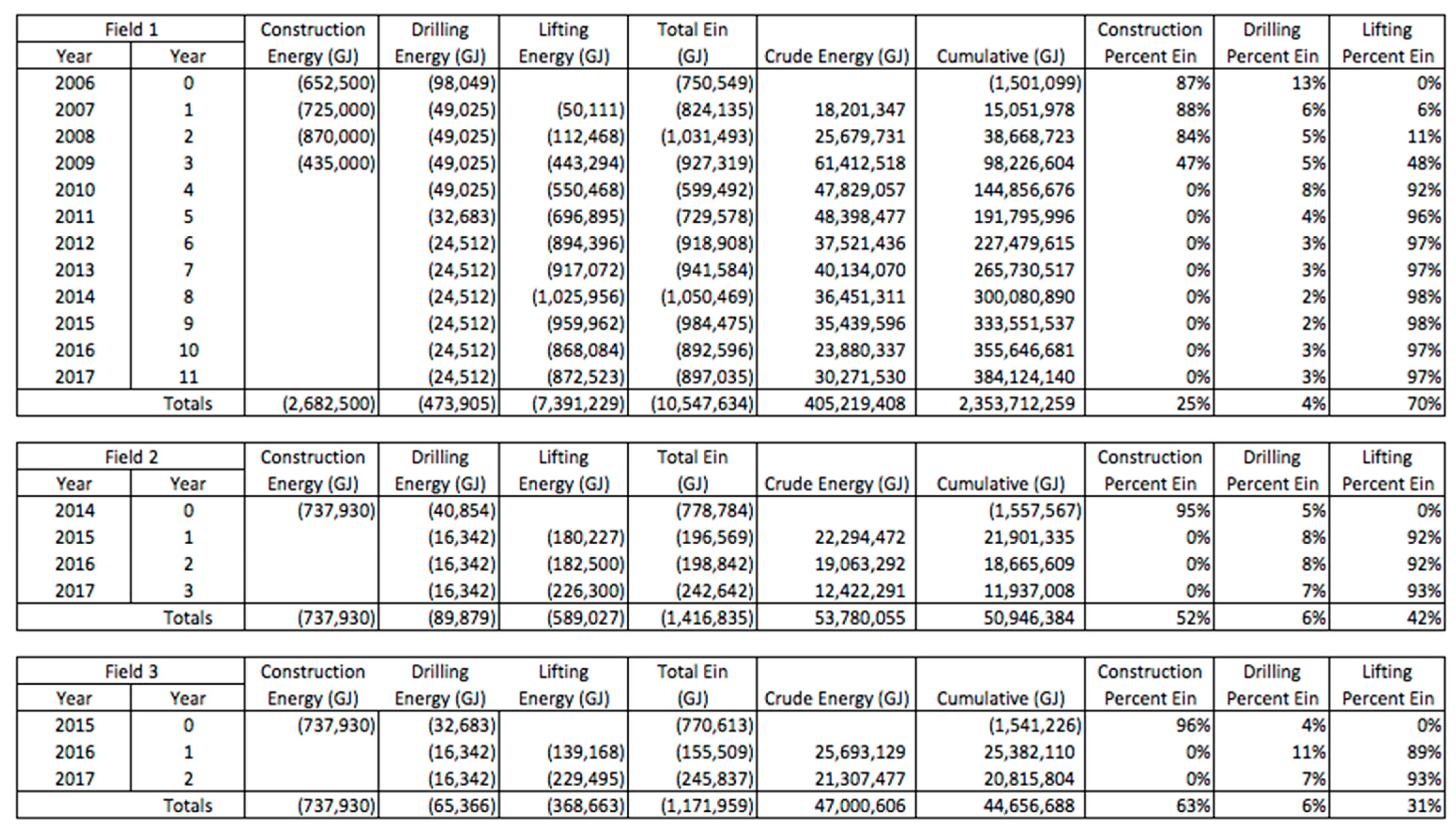
As can described in Appendix A, Figure A3, the drilling energies’ share of the yearly energy-in for Field 1 ranges from 13% in early life to approximately 3% in late life, as the drilling rate decreases. Drilling energy for Fields 2 and 3 as a percentage of the yearly energy applied ranges from 11% to 5%. Construction energy as a percentage of the total applied over the entire field life ranged from 25% for Field 1, the oldest field, to 63% for Field 3, the newest field. All fields experience the energy breakeven point within the first year of production. This is due to the large quantity of energy produced during the early high crude oil production rates.
Overall, there is greater confidence in the EROI-1dLifting results compared to the EROIs that consider drilling and construction. This is due to the fact that actual fuel consumption on the platforms is a well-known quantity, while drilling energy and construction energy employed less certain energy consumption assumptions.
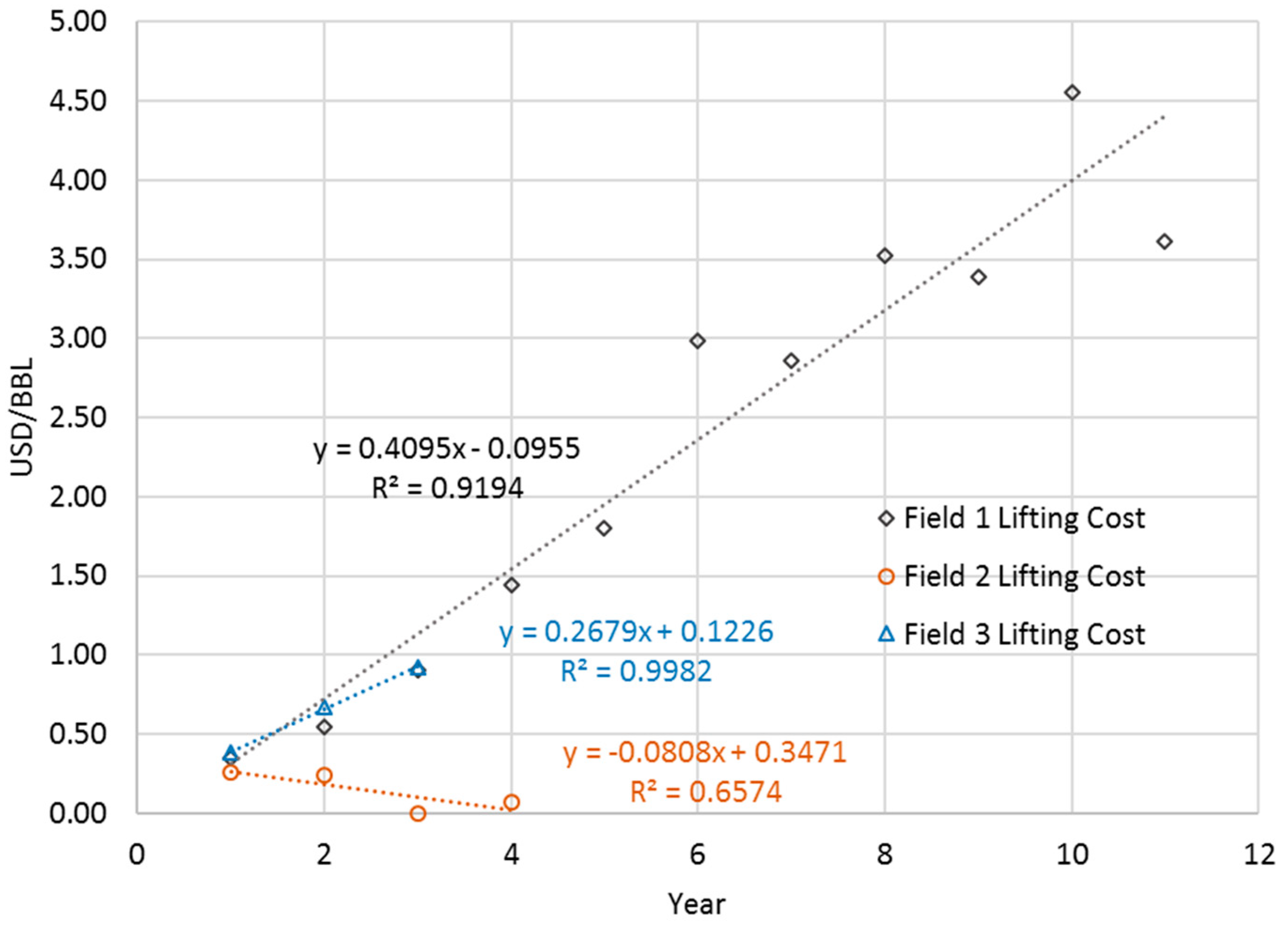
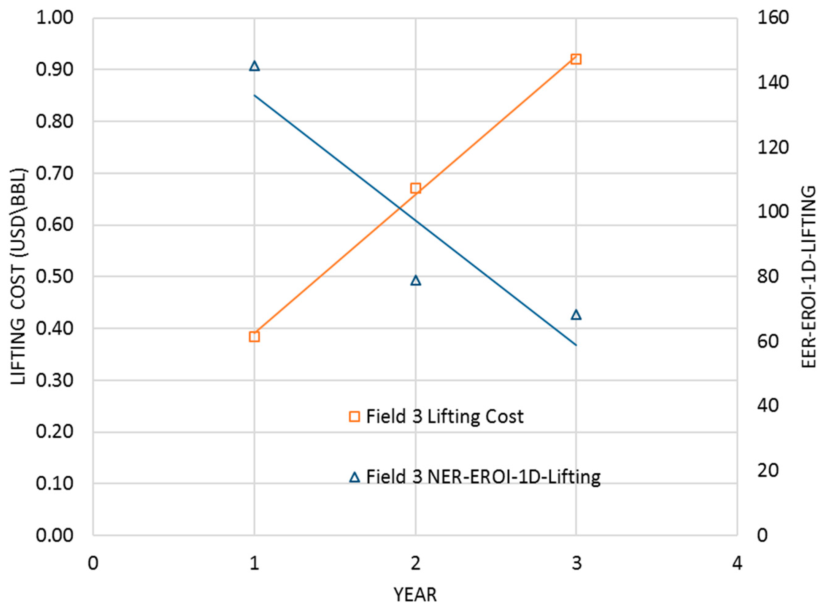
It is proposed that there is great insight that can be gained by understanding the relationship between EROI-1dLifting and lifting costs. Lifting costs trends are shown in Figure 9 for Fields 1, 2, and 3. The lifting cost of Field 1 increases at a higher rate than Field 3 due to the fact that Field 1 runs exclusively on imported diesel fuel, while Field 3 runs on a combination of imported diesel fuel and “free” produced natural gas. Field 2, which runs primarily on associated gas, actually shows a decreasing trend, as the operational team have focused on minimizing the use of diesel fuel in the field.
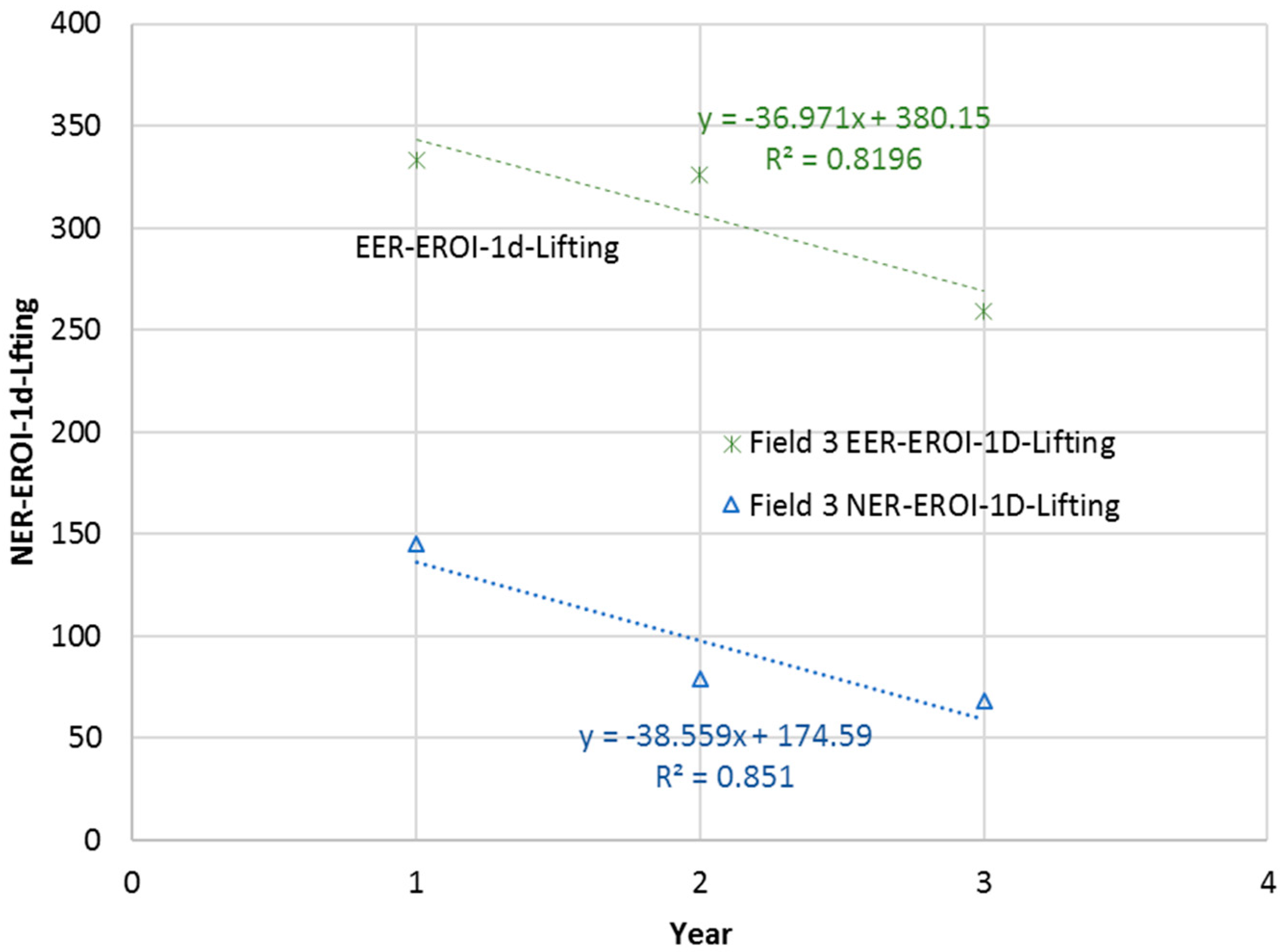
Field 3 was selected for comparison between NER- EROI-1dLifting and EER- EROI-1dLifting, since Field 3 generators run on a combination of diesel fuel and natural gas, commonly referred to as “dual fuel” engines. As indicated in Figure 10, the EROIs for Field 3 are significantly higher when only external fuel is accounted.
3. Material and Methods
Three small offshore fields were developed as case studies. Each field’s peak production was under 25,000 barrels of oil per day, and as such are classified as non-giant fields. Each field has been in operation for between 3 and 12 years. Each field employs artificial lifting of reservoir fluids utilizing downhole electrical submersible pumps (ESPs) and employs conventional surface centrifugal pumps to pressurize and inject, or dispose of, the associated produced water. Power required for the ESPs and the surface water injection pumps represent more than 80% of each platform’s total platform power demand.
ESP systems are composed of two subsystems, electrical and hydraulic. The electrical system is composed of an electrical power source, surface equipment (motor controllers and transformers), cables, and the ESP motor itself, which is located in the well, beneath the pump. The hydraulic subsystem is composed of the pump and the discharge piping, which traverses up the well to the offshore platform.
The processing requirements on the platform are minimal and include only separation of reservoir fluids into oil, water, and gas by gravity, crude stabilization by flashing at low pressure, and water treatment with the use of cyclonic devices driven by a small pressure gradient between the production separator and the water degassing vessel.
Reciprocating internal combustion engine generators are installed on each platform and generally consume either diesel fuel or natural gas, although several diesel generators are equipped with dual fuel systems, which allows for the produced natural gas to supplement the imported diesel fuel. Additional characteristics of the three fields are described in Table 6.
The method employed in this research is comprised of the following main steps:
- Gather energy inputs and outputs for three small offshore fields;
- Calculate time series EROI-1d values for each field;
- Apply regression analysis to the time series data where appropriate;
- Calculate lifting costs for three small offshore fields;
- Analysis of results.
3.1. Energy Outputs
Energy outputs are derived by converting the average daily crude production rate for each year to an energy rate using typical lower heating values for crude of 6.1 GJ/barrel.
3.2. Energy Input—Lifting Energy
Lifting energy is calculated by converting fuel consumption rates to energy equivalents using the lower heating value. For Fields 1, 2, and 3, the average daily diesel consumption for each platform, which is recorded in US gallons per day, is converted to an average daily energy rate by using a lower heating value of 146 MJ per US gallon. For Fields 2 and 3, the average daily natural gas consumption recorded in million standard cubic feet per day (MMSCFD) is converted to an average daily energy rate using a heating value of 1.0 MJ per standard cubic foot.
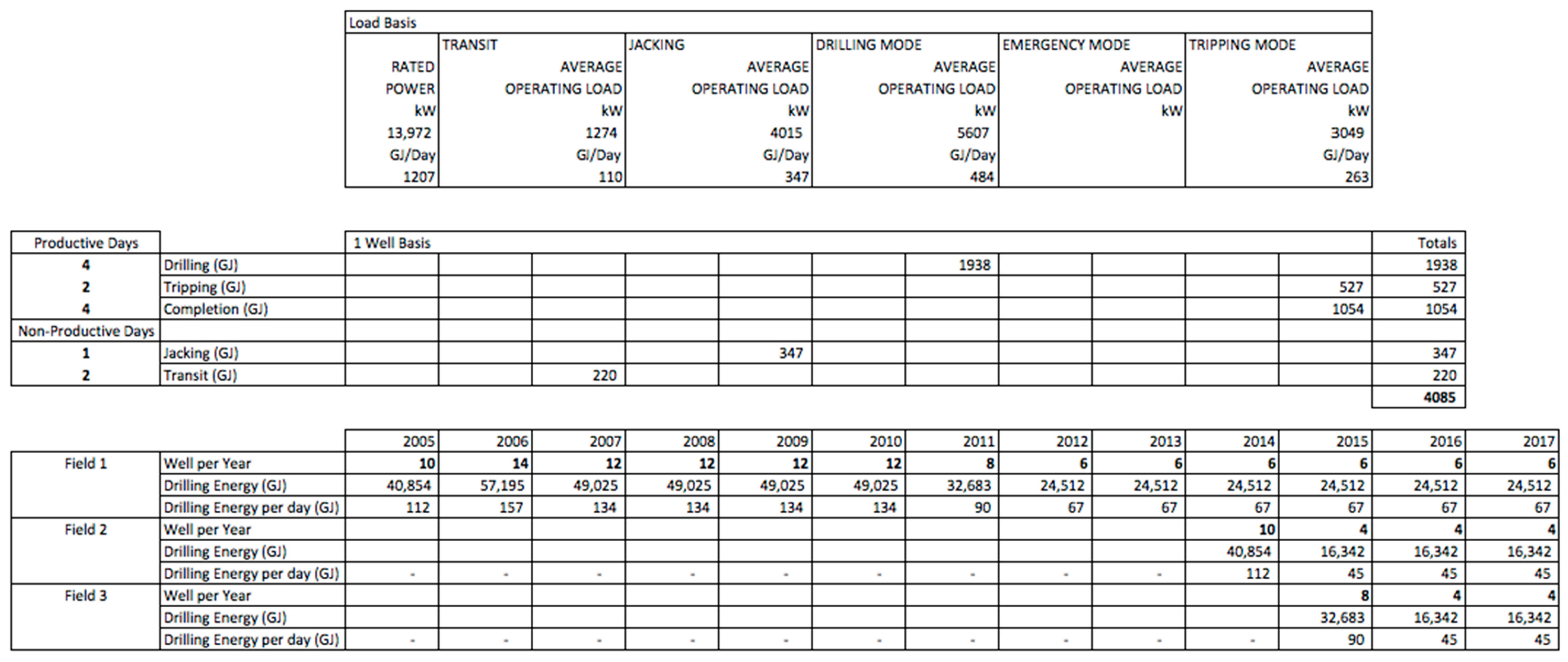
3.3. Energy Input—Drilling Energy
The reservoirs are highly compartmentalized. The exploitation strategy for this type of reservoir generally requires numerous wells; therefore, there is continuous drilling of new wells in the annual drilling campaign. The high level of drilling activity is required to sustain production on each platform. As such, the energy consumed by the annual drilling program was calculated based on an estimate of the historical number of wells drilled per year and an estimated drilling rig power load for each well.
3.4. Energy Input—Construction Energy
Finally, construction and installation of offshore platforms is an energy intensive process. For large capital expenditures, it is common place to convert capital expenditures to energy consumption values using published energy intensities for heavy industry. For platform construction, an energy intensity value of 14 MJ/USD (2005 USD basis) was applied, which is consistent with published data. Construction energy was amortized for three years following initial production. All platform costs were converted to 2005 dollars, which is aligned with the energy intensity value applied.
3.5. Derivation of EROI-1d
With the energy inputs and energy outputs derived, several time series for EROI-1ds of interest were developed for each field. For all fields, EROI-1d-NER was calculated. For Field 3. both EROI-1d-NER and EROI-1d-EER were calculated, since the field employs both external and internal fuel sources.
3.6. Lifting Cost
Lifting costs were calculated by converting the annual daily diesel fuel consumption to an average daily cost using a diesel fuel cost of 3.0 USD per US gallon. A representative cost was selected and no attempt was made to account for market fluctuations in diesel fuel cost.
4. Conclusions
This study demonstrates the benefits to oil field analysts of applying the EROI methodology. This is established with respect to the examination of the energetic behavior of three small offshore fields. It is clear that the EROI methodology can be used to aggregate energy information in order to provide insight into the energetic, valued-added nature of a development, which is not as readily understood when the underlying information is dispersed and generally disconnected, such as with regards to production profiles, utility tables, drilling schedule, construction reports, etc. Conversely, this study reveals that the EROI methodology can also be used to dissect energy information to illuminate particular aspects of the development, such as with respect to lifting energy, which is known to be a significant components of the total energy consumed by oil fields and a key influencer of the variable costs. The following conclusions can be drawn from this research:
- All three fields indicate a steeply declining EROI-1d trend. The EROI-1dLifting decline can be directly attributed to the lifting process becoming more energy intensive over time. This applies equally to Field 1, despite the fact that the recovery method was changed, employing low pressure water disposal rather than high pressure water injection. Without the change in recovery strategy, the EROI-1dLifting trend would have declined more steeply from 2011 onwards.
- The decreasing EROI-1d trend also holds true for the EROI-1dLifting+Drilling and for the EROI-1dLifting+Drilling+Construction parameters, but to a lesser extent, since (1) drilling energy intensity decreases after the initial production wells are drilled, and (2) the methodology used amortized the construction energy evenly over the first three years of production.
- Production decline modeling in an oilfield is an intensely studied topic. Energy return decline modeling generally receives very little attention, and is therefore not as well understood. It is suggested that more vigorous efforts should be made to understand the EROI decline behavior of oilfields, since it has a direct impact on the efficiency and economics of the field, even more so than the production decline.
- Drilling and construction energies constitute a substantial component of the total energy consumption. The drilling contribution to energy consumption is related to the drilling intensity over the life of the field, which usually starts with a large number of initial development wells and then tapers off to a lesser number of wells per year later in the field life. Construction energy, on the other hand, is completely expended just prior to first production. The energy breakeven point was found to occur within the first year of production for all three fields, due to the large energy gains obtained by early high production rates.
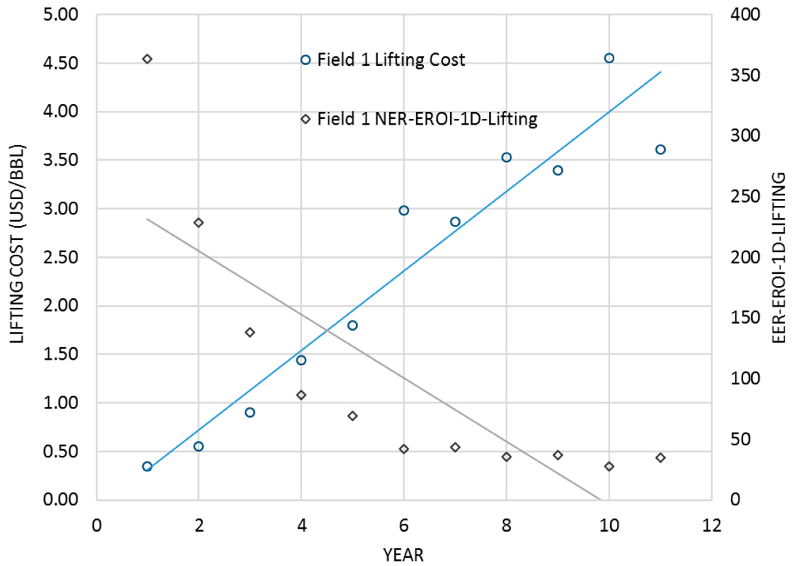
- EROI-1dLifting and lifting costs are found to be inversely related, since the input energy has a cost, such as the cost of diesel fuel. The magnitude of the lifting cost and the degree by which lifting costs increase over time depends on the mix of fuels used, which can range from complete reliance on procured diesel fuel (Field 1) to total fuel self-sufficiency when sufficient quantities and quality of internally derived natural gas are available (Field 2). In between these two extremes is the case where there is a mixture of internal and external fuels sources applied (Field 3).
- This method describes a more rigorous approach to understanding and estimating lifting costs and highlights the impact on costs of the source of energy consumptions with respect to internal vs. external.
4.1. Limitations of This Work
The energetic analysis of three offshore small fields as case studies is revealing, but may not be representative of the numerous small fields scattered across the world. The diversity of small fields is enormous. Each small field has identifying qualities, such as the location (e.g., offshore vs. onshore), environment (e.g., tropical, desert, or artic), number and capacity of wells, the drilling complexity of the wells, the crude oil properties, the crude production rate profile, the associated water profile, and the associated gas qualities and quantities. One of the most important distinguishing elements of a small field is the recovery strategy (e.g., primary, secondary, or tertiary), and the lifting mechanism (e.g., natural flow, sucker-rod pumps, electrical submersible pumps, progressive cavity pumps, gas lift, etc.). All of these variables will have an impact on the energy profile of a particular small field.
Furthermore, the relationships explored in this research are in some cases limited by the span of field data available. Fields 2 and 3 are relatively young developments, with only 3 and 4 years of data available, respectively. The results of the regression analysis, therefore, must be considered preliminary and the continued monitoring of these fields is required to truly understand the trends and project future EROI and lifting costs.
The conversion of construction costs to energy has an unknown degree of error due to the accuracy of the energy intensity factor employed, which may not be representative of the region or of local construction practices. The intention was to provide an order of magnitude estimate only for construction energy of the three fields studied.
In spite of these limitation, the intention of this research is to illuminate a more detailed EROI methodology, describe the energetic behavior of three somewhat typical fields, and most importantly to highlight the value of employing detailed energy accounting to development teams managing small fields.
4.2. Future Work
It is suggested that future work should revolve around the development of mathematical models to describe EROI decline trends and associated lifting costs. Another suggested area of future work is related to the development of an EROI-centered methodology for improving lifting cost estimates during concept evaluations. As such, concept evaluations could test EROI and lifting costs sensitivities with respect to recovery methods and fuel sources. Finally, it is suggested that the energetic behavior of small fields can be analyzed with respect to understanding the common energetic patterns linked to the recovery method.
Author Contributions
Conceptualization, D.G. and D.O.; methodology, D.G. and D.O.; investigation, D.G.; writing—original draft preparation, D.G.; writing—review and editing, D.O.; visualization, D.G.; supervision, D.O.
Funding
This research received no external funding.
Conflicts of Interest
The authors declare no conflict of interest.
Appendix A
Figure A1.
Drilling Energy Calculation.

Figure A2.
Construction Energy Calculation.
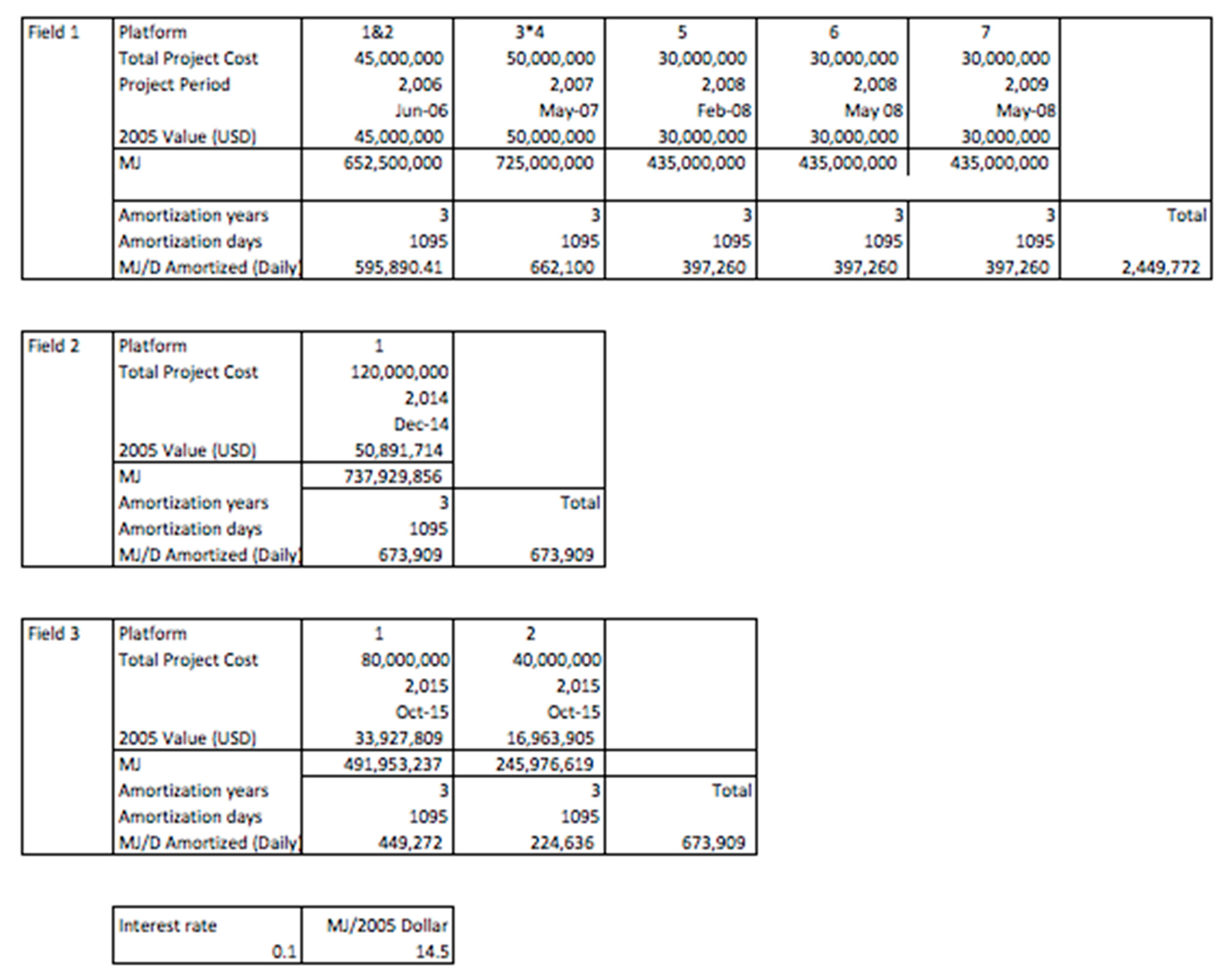
Figure A3.
Energy Breakeven Calculation.

References
- Höök, M.; Hirsch, R.; Aleklett, K. Giant oil field decline rates and their influence on world oil production. Energy Policy 2009, 37, 2262–2272. [Google Scholar] [CrossRef] [Green Version]
- Sorrell, S.; Speirs, J.; Bentley, R.; Miller, R.; Thompson, E. Shaping the global oil peak: A review of the evidence on field sizes, reserve growth, decline rates and depletion rates. Energy 2012, 37, 709–724. [Google Scholar] [CrossRef]
- Bullard, C.W., III; Herendeen, R.A. The energy cost of goods and services. Energy Policy 1975, 3, 268–278. [Google Scholar] [CrossRef]
- Herendeen, R.A.; Cleveland, C. Net energy analysis: Concepts and methods. Encycl. Energy 2004, 4, 283–289. [Google Scholar]
- King, C.W.; Hall, C.A. Relating financial and energy return on investment. Sustainability 2011, 3, 1810–1832. [Google Scholar] [CrossRef]
- Cleveland, C.J. Energy quality and energy surplus in the extraction of fossil fuels in the US. Ecol. Econ. 1992, 6, 139–162. [Google Scholar] [CrossRef]
- Cleveland, C.J. Net energy from the extraction of oil and gas in the United States. Energy 2005, 30, 769–782. [Google Scholar] [CrossRef]
- Gagnon, N.; Hall, C.A.; Brinker, L. A preliminary investigation of energy return on energy investment for global oil and gas production. Energies 2009, 2, 490–503. [Google Scholar] [CrossRef]
- Dale, M.; Krumdieck, S.; Bodger, P. Net energy yield from production of conventional oil. Energy Policy 2011, 39, 7095–7102. [Google Scholar] [CrossRef]
- Grandell, L.; Hall, C.A.; Höök, M. Energy return on investment for Norwegian oil and gas from 1991 to 2008. Sustainability 2011, 3, 2050–2070. [Google Scholar] [CrossRef]
- Brandt, A.R. Oil depletion and the energy efficiency of oil production: The case of California. Sustainability 2011, 3, 1833–1854. [Google Scholar] [CrossRef]
- Guilford, M.C.; Hall, C.A.; O’Connor, P.; Cleveland, C.J. A new long term assessment of energy return on investment (EROI) for US oil and gas discovery and production. Sustainability 2011, 3, 1866–1887. [Google Scholar] [CrossRef]
- Murphy, D.J.; Hall, C.A.; Dale, M.; Cleveland, C. Order from chaos: A preliminary protocol for determining the EROI of fuels. Sustainability 2011, 3, 1888–1907. [Google Scholar] [CrossRef]
- Cleveland, C.J.; O’connor, P.A. Energy return on investment (EROI) of oil shale. Sustainability 2011, 3, 2307–2322. [Google Scholar] [CrossRef]
- Poisson, A.; Hall, C.A. Time series EROI for Canadian oil and gas. Energies 2013, 6, 5940–5959. [Google Scholar] [CrossRef]
- Nogovitsyn, R.; Sokolov, A. Preliminary Calculation of the EROI for the Production of Gas in Russia. Sustainability 2014, 6, 6751–6765. [Google Scholar] [CrossRef] [Green Version]
- Brandt, A.R.; Sun, Y.; Bharadwaj, S.; Livingston, D.; Tan, E.; Gordon, D. Energy return on investment (EROI) for forty global oilfields using a detailed engineering-based model of oil production. PLoS ONE 2015, 10, e0144141. [Google Scholar] [CrossRef]
- Brandt, A.R.; Yeskoo, T.; Vafi, K. Net energy analysis of Bakken crude oil production using a well-level engineering-based model. Energy 2015, 93, 2191–2198. [Google Scholar] [CrossRef] [Green Version]
- Tripathi, V.S.; Brandt, A.R. Estimating decades-long trends in petroleum field energy return on investment (EROI) with an engineering-based model. PLoS ONE 2017, 12, e0171083. [Google Scholar] [CrossRef]
- Court, V.; Fizaine, F. Long-term estimates of the energy-return-on-investment (EROI) of coal, oil, and gas global productions. Ecol. Econ. 2017, 138, 145–159. [Google Scholar] [CrossRef]
- Feng, J.; Feng, L.; Wang, J. Analysis of Point-of-Use Energy Return on Investment and Net Energy Yields from China’s Conventional Fossil Fuels. Energies 2018, 11, 313. [Google Scholar] [CrossRef]
- Brandt, A.R.; Yeskoo, T.; McNally, M.S.; Vafi, K.; Yeh, S.; Cai, H.; Wang, M.Q. Energy intensity and greenhouse gas emissions from tight oil production in the bakken formation. Energy Fuels 2016, 30, 9613–9621. [Google Scholar] [CrossRef]
- Hall, C.A.; Balogh, S.; Murphy, D.J. What is the minimum EROI that a sustainable society must have? Energies 2009, 2, 25–47. [Google Scholar] [CrossRef]
- Pashakolaie, V.G.; Khaleghi, S.; Mohammadi, T.; Khorsandi, M. Oil production cost function and oil recovery implementation-evidence from an iranian oil field. Energy Explor. Exploit. 2015, 33, 459–470. [Google Scholar] [CrossRef]
- Stermole, F.J.; Kifer Ten Eyck, D. Cost Per Barrel as an Economic Decsion Tool. Soc. Pet. Eng. J. SPE-16994-MS. 1987. Available online: https://www.onepetro.org/general/SPE-16994-MS (accessed on 17 July 2019).
- Martinez, R.E. Forecast Techniques for Lifting Cost in Gas and Oil Onshore Fields. In Proceedings of the SPE Latin American and Caribbean Petroleum Engineering Conference, Buenos Aires, Argentina, 25–28 March 2001. [Google Scholar]
- Brundred, L.L. Economics of Water Flooding. J. Pet. Technol. 1954. [Google Scholar] [CrossRef]
- Cobb, W.; Marek, F. Determination of volumetric sweep efficiency in mature waterfloods using production data. In Proceedings of the SPE Annual Technical Conference and Exhibition, San Antonio, TX, USA, 5–8 October 1997. [Google Scholar]
- Alhuthali, A.; Oyerinde, A.; Datta-Gupta, A. Optimal waterflood management using rate control. SPE Reserv. Eval. Eng. 2007, 10, 539–551. [Google Scholar] [CrossRef]
- Chang, H.L. Polymer flooding technology yesterday, today, and tomorrow. J. Pet. Technol. 1978, 30, 1113–1128. [Google Scholar] [CrossRef]
- Sheng, J.J.; Leonhardt, B.; Azri, N. Status of polymer-flooding technology. J. Can. Pet. Technol. 2015, 54, 116–126. [Google Scholar] [CrossRef]
- Kumar, S.; Mandal, A. A comprehensive review on chemically enhanced water alternating gas/CO2 (CEWAG) injection for enhanced oil recovery. J. Pet. Sci. Eng. 2017, 157, 696–715. [Google Scholar] [CrossRef]
- Afzali, S.; Rezaei, N.; Zendehboudi, S. A comprehensive review on enhanced oil recovery by water alternating gas (WAG) injection. Fuel 2018, 227, 218–246. [Google Scholar] [CrossRef]
- Santos, R.; Loh, W.; Bannwart, A.; Trevisan, O. An overview of heavy oil properties and its recovery and transportation methods. Braz. J. Chem. Eng. 2014, 31, 571–590. [Google Scholar] [CrossRef] [Green Version]
- Keplinger, C. Economic Considerations Affecting Steam Flood Prospects. In Proceedings of the Symposium on Petroleum Economics and Evaluation, Dallas, TX, USA, 8–9 February 1965. [Google Scholar]
- McCarthy, D.W.; Groat, C.; Chen, J.-K.; Liau, T.-H.; Weaver, R.E.; Aldahir, A. Tertiary Oil Recovery Economics in Louisiana. In Proceedings of the SPE/DOE Enhanced Oil Recovery Symposium, Tulsa, OK, USA, 3–5 April 1981. [Google Scholar]
- Chaar, M.; Venetos, M.; Dargin, J.; Palmer, D.B. Economics of steam generation for thermal EOR. In Proceedings of the Abu Dhabi International Petroleum Exhibition and Conference, Abu Dhabi, UAE, 10–13 November 2014. [Google Scholar]
- Aseeri, A.S. How Much is Steam Worth? In Proceedings of the Abu Dhabi International Petroleum Exhibition & Conference (ADIPEC), Abu Dhabi, United Arab Emeriates, 13–16 November 2017. [Google Scholar]
- Gordon, D.; Brandt, A.R.; Bergerson, J.; Koomey, J. Know Your Oil: Creating a Global Oil-Climate Index; Carnegie Endowment for International Peace: Washington, DC, USA, 2015. [Google Scholar]
Figure 1.
Field 1 Production vs. NER-1d-EROILifting.
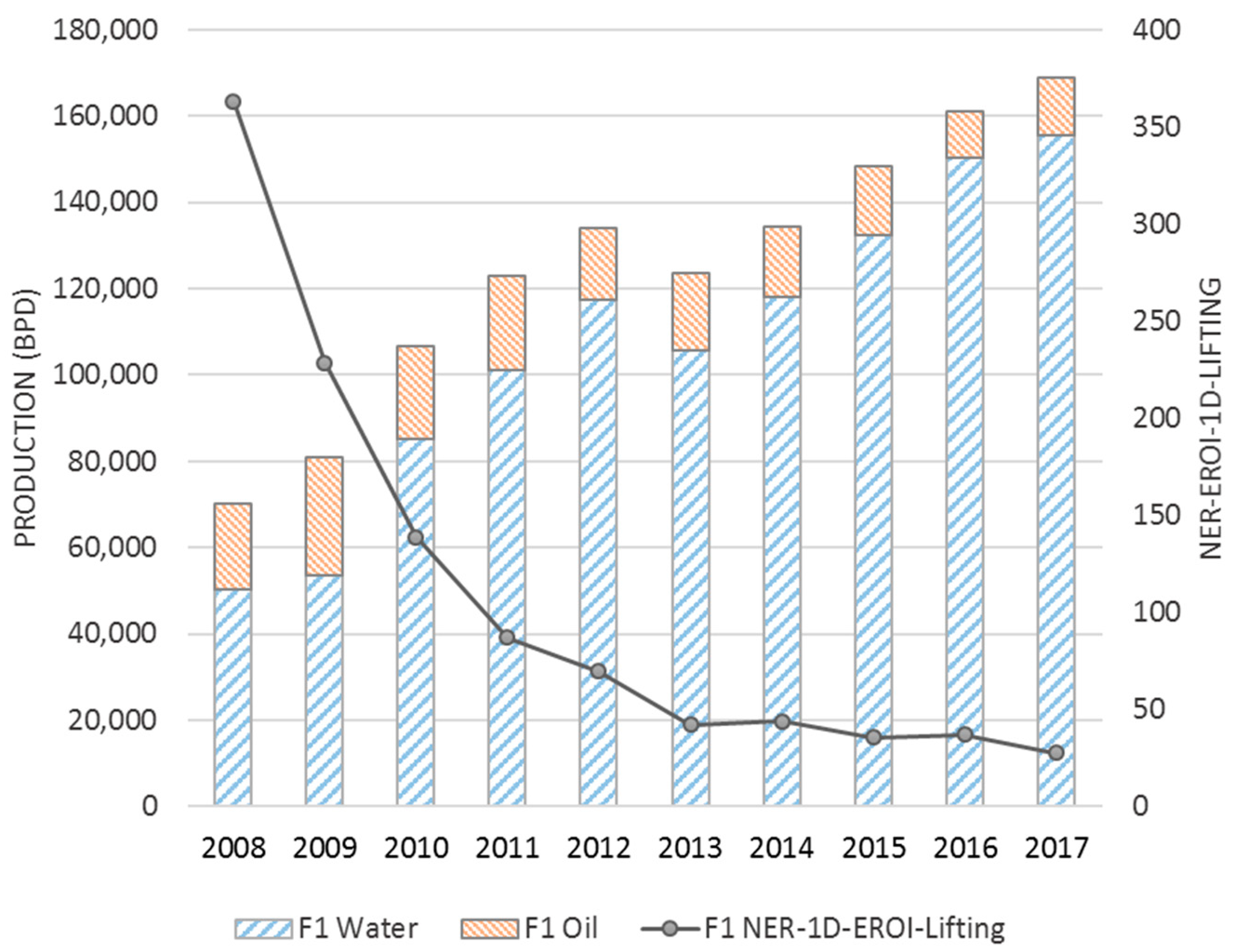
Figure 2.
Field 2 Production vs. NER-1d-EROILifting.
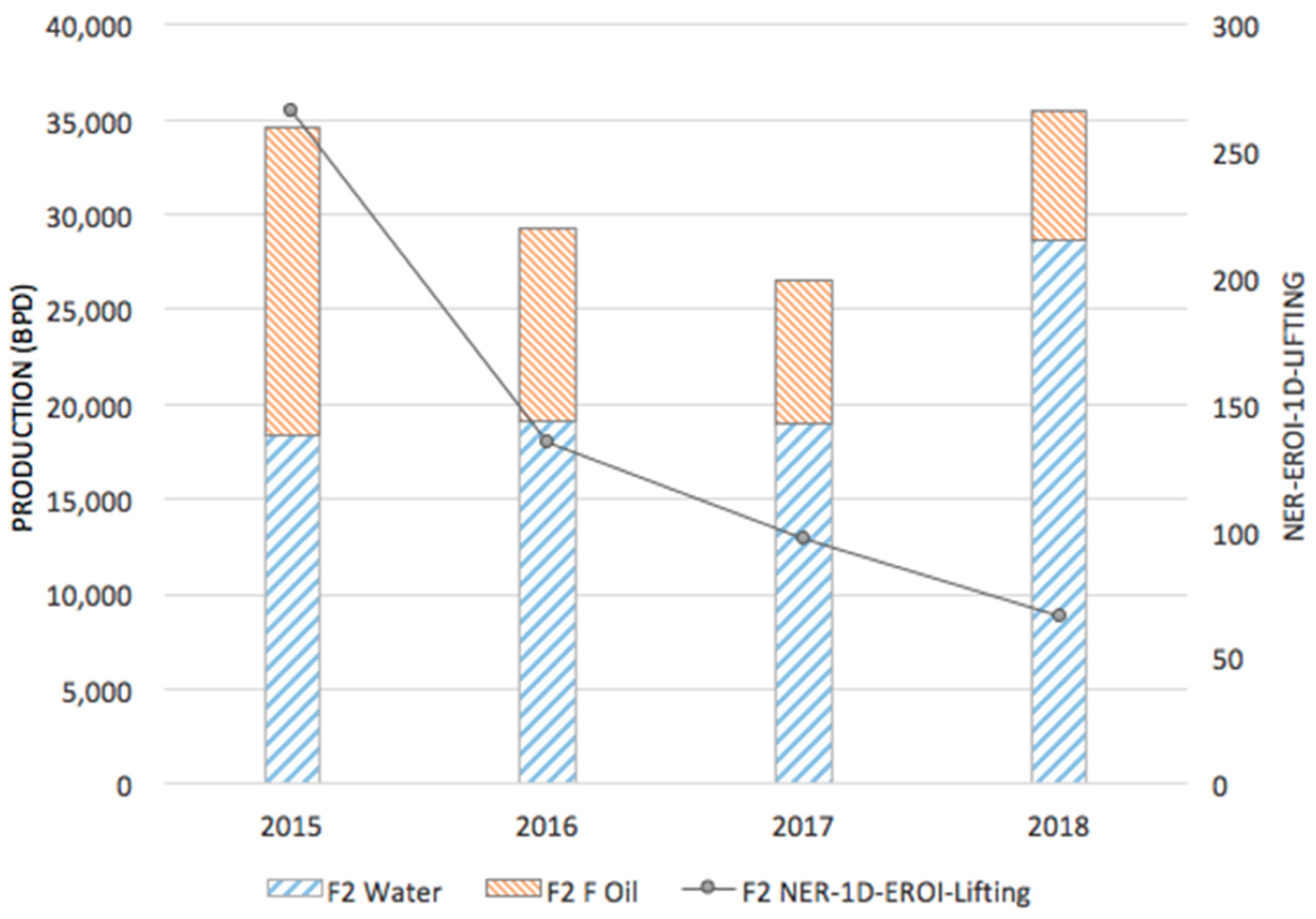
Figure 3.
Field 3 Production vs. NER-1d-EROILifting.
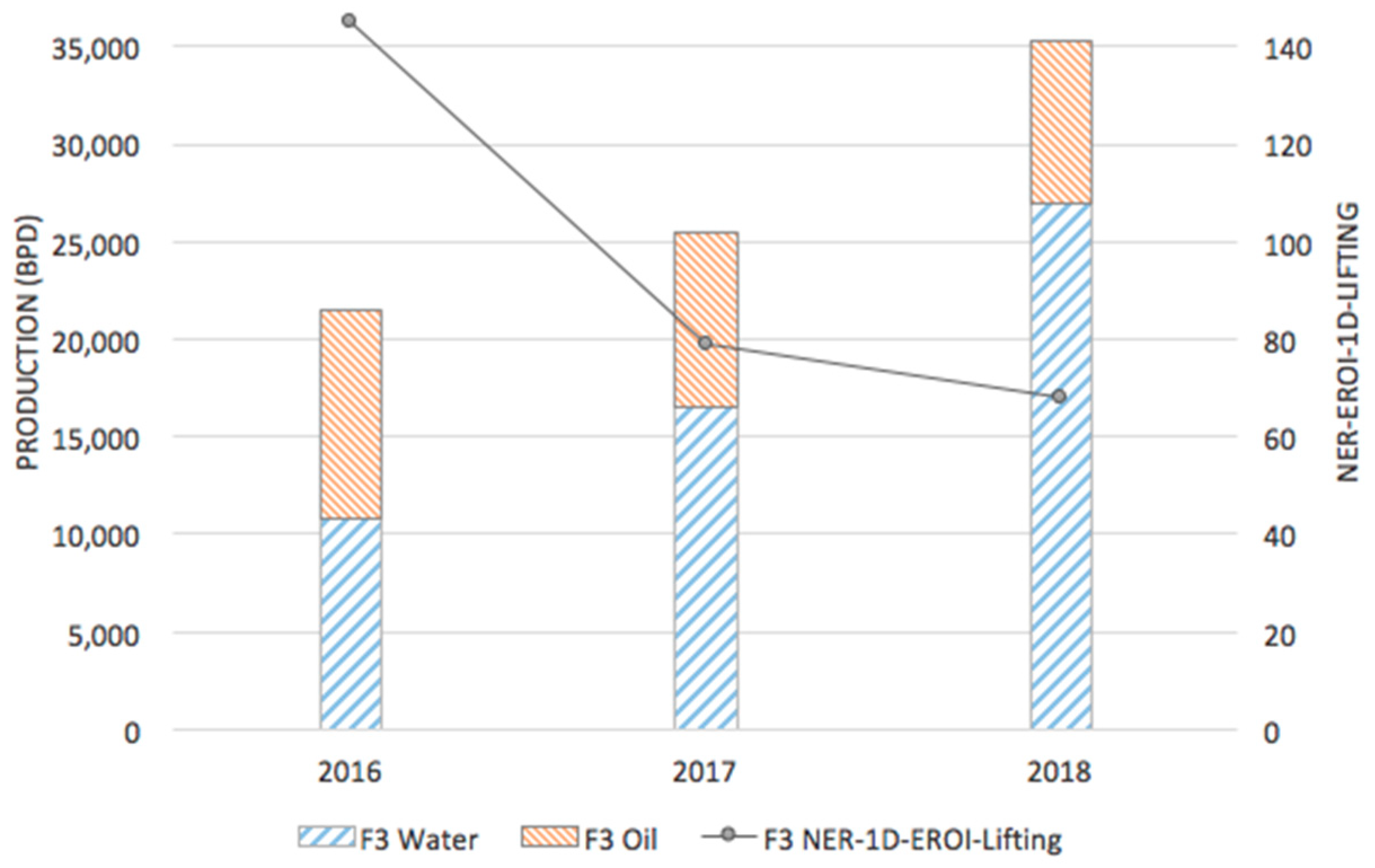
Figure 4.
NER-EROI-1dLifting time series for three small fields.

Figure 5.
NER-EROI-1dLifting regression analysis (linear).

Figure 6.
NER-EROI-1dLifting regression analysis (exponential).
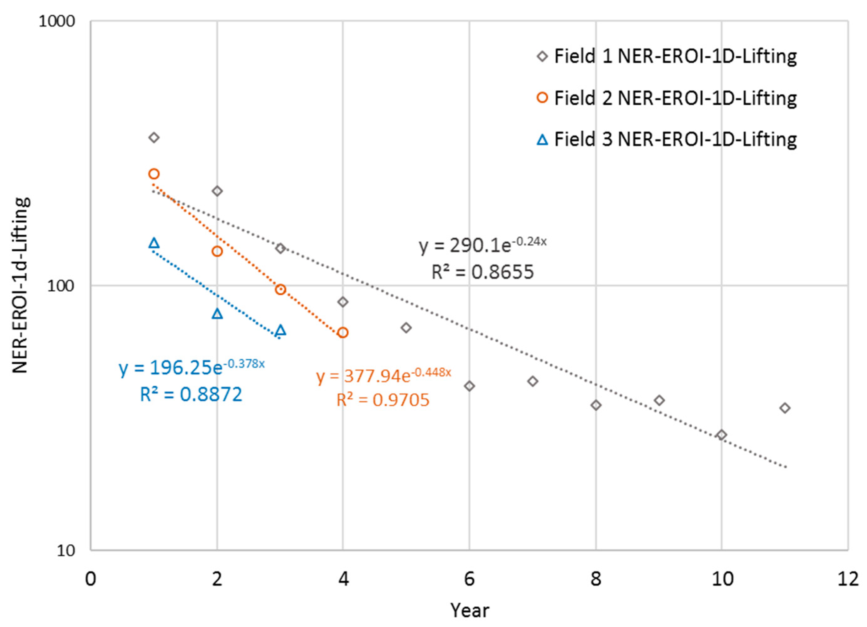
Figure 7.
NER-EROI-1dLifting+Drilling for three fields.

Figure 8.
NER-EROI-1dLifting+Drilling+Construction for three fields.

Figure 9.
Comparison of lifting costs between Fields 1, 2, and 3.

Figure 10.
Comparison of NER-EROI-1dLifting vs. EER-EROI-1dLifting for Field 3.

Figure 11.
Lifting Costs and NER-EROI-1dLifting vs. Time for Field 1.

Figure 12.
Lifting Costs and NER-EROI-1dLifting vs. Time for Field 3.


Table 1.
EROI Boundaries.
| Boundaries | Extraction (1) | Processing (2) | End-Use (3) | |
|---|---|---|---|---|
| 1 | Direct energy and materials | EROI 1d | EROI 2d | EROI 3d |
| 2 | Indirect energy and materials input | EROI standard | EROI 2i | EROI 3i |
| 3 | Indirect labor consumption | EROI 1lab | EROI 2lab | EROI 3lab |
| 4 | Auxiliary services consumption | EROI 1aux | EROI 2aux | EROI 3aux |
| 5 | Environmental | EROI 1env | EROI 2env | EROI 3env |
Table 2.
EROI-1D Sub-parameters.
| Sub-Parameter of EROI-1d | Purpose |
|---|---|
| EROI-1dLifting | The Energy Return on Investment for Direct Energies and Materials related to lifting only, which is the incremental energy required to produce a barrel of crude oil. Used to understand lifting energy breakeven points and lifting costs |
| EROI-1dLifting+Drilling | The Energy Return on Investment for Direct Energies and Materials related to lifting and the drilling of wells. Used to understand the main continuous direct energy consumers during the life of the field, post construction phase. |
| EROI-1dLifting+Drilling+Construction | The Energy Return on Investment for Direct Energies and Materials related to lifting, drilling and construction of surface facilities. The original intention of EROI-1d, which includes all direct energy and materials. |
Table 3.
Summary of EROI findings.
| Year Published | Author/s | Subject | Boundaries and Method | EROI Range, Trend, and Period |
|---|---|---|---|---|
| 1992 | Cutler | EROI methodology described, including quality corrections based on thermal equivalents and other measures. Time series for petroleum and coal production in the United States. | Sector: U.S. petroleum Method: Top-Down Extraction only by converting direct costs to energies. | EROI: 10 to 15 Trend: Indiscernible/Fluctuating Period: 1954 to 1984 |
| 2001 | Cutler | EROI methodology described with further consideration of quality issues. EROI time series for U.S. petroleum sector. | Sector: U.S. petroleum. Method: Top-Down Extraction only by converting direct costs to energies. | EROI: 16 to 24 Trend: Indiscernible/Fluctuating Period: 1954 to 1994 |
| 2009 | Gagnon et al. | EROI time series of global oil and gas production. Method includes converting published costs to energy inputs. | Sector: Global petroleum. Method: Top-down based on published production rates and costs. | EROI: 25 to 20. Trend: Declining. Period: 1992 to 2006 |
| 2011 | Dale et al. | EROI and Net Energy Yield (NEY) concept and methodology. | Case studies not included. | - |
| 2011 | Grandell et al. | EROI time series for Norwegian oil and gas sector. | Sector: Norwegian petroleum. Method: Hybrid based on published production rates and costs. Takes into account specific fuel consumption data collected by the Norwegian authorities. | EROI: 40 to 57. Trend: Fluctuating. Period: 1991 to 2007 |
| 2011 | Brandt | Introduces variants of EROI regarding Net Energy Return and External Energy Return. EROI time series for California oil and gas production. | Sector: California petroleum. Method: Hybrid Based on published production rates and costs. Differentiates between EER and NER. | NER-EROI: 65 to 10. Trend NER: Decreasing. Period: 1950 to 2010. EER-EROI: 90 to 8. Trend NER: Decreasing. Period: 1950 to 2010 |
| 2011 | Guilford | Long-term assessment of U.S. oil and gas production EROI. | Sector: U.S. petroleum. Method: Top-down. | EROI: 24 to 15. Trend: Fluctuating/Decreasing. Period: 1920 to 2010 |
| 2011 | Murphy et al. | Discussion on a refined methodology covering boundaries and EROI subdivisions. | Case studies not included. | - |
| 2011 | Cleveland and O’Connor | Analysis of EROI of Oil Shale in the United States. | Sector: U.S. Oil Shale. Method: Hybrid | EROI: 1.4 to 2. Trend: Single Point Estimate. Period: 2010 |
| 2013 | Poisson and Hall | EROI time series analysis for Canadian oil and gas production | Sector: Canadian petroleum. Method: Top-down. Separates direct and indirect energies. | Direct energy only EROI: 17 to 14. Trend: Declining. Period: 1990 to 2010. Direct and Indirect EROI: 15 to 12. Trend: Declining. Period: 1990 to 2010 |
| 2014 | Nogovitsyn and Sokolov | EROI time series analysis for overall Russian hydrocarbon production, with a separate analysis for gas production by major fields. | Sector: Russian petroleum. Method: Top-down for overall hydrocarbon, hybrid for field-specific estimates. All estimates include transportation. | Hydrocarbons EROI: 36–30. Trend: Declining. Period: 2005 to 2012. Gas EROI: Point estimates of Gas only EROIs for specific fields range from 70 to 129. Period: 2010 to 2013 |
| 2015 | Brandt et al. | NER-EROI and EER-EROI based on detailed field-level engineering analysis using published data. | Sector: Forty specific global fields. Method: Hybrid. Engineering review includes a detailed analysis taking into account thermal EOR properties, lifting energies, drilling energy intensities, as well as processing practices. | NER-EROI total: 122 to 18. NER-EROI oil only: 120 to 5. Trend: Point estimates for 2015. Period: 2015 |
| 2017 | Tripathi and Brandt | Boundary model expanded. NER-EROI and EER-EROI time series for six major oil and gas fields. | Sector: Six specific fields: Cantarell, Forties, Midway-Sunset, Prudhoe Bay, and Wilmington fields. Method: Hybrid. Engineering review, includes a detailed analysis considering production method, field properties, fluid properties, production and processing practices, and transportation. | Field: Cantarell. NER-EROI total: 72 to 5. Trend: Decreasing. Period: 1978 to 2012. Field: Forties. NER-ERO total: 28 to 16. Trend: Decreasing. Period: 1974 to 1999. Field: Midway-Sunset. NER-ERO total: 12 to 3. Trend: Decreasing. Period: 1965 to 2007. Field: Prudhoe Bay. NER-ERO total: 19 to 6. Trend: Decreasing. Period: 1977 to 2004. Wilmington fields NER-EROI total: 60 to 12. Trend: Decreasing. Period: 1955 to 2007 |
Table 4.
Summary of Case Studies.
| Field | Water Depth | Production Period Evaluated | Processing Requirements | Lifting Mechanism | Recovery Method | Fuel |
|---|---|---|---|---|---|---|
| Field 1 | 60 m | 2008 to 2018 | Crude/water/gas separation, crude stabilization, and associated water treatment and disposal. | Electrical Submersible Pumps (ESPs) | Initially secondary recovery, employing water injection at > 1000 pounds per square inch (psi) at the wellhead. In 2012. the field switched to primary recovery, with associated (produced) water disposal at low pressure <300 psig. | Exclusively diesel since the gas produced is of insufficient quality and quantity (High CO2) (100% diesel) |
| Field 2 | 55 m | 2015 to 2018 | Crude/water/gas separation, crude stabilization, associated water treatment and injection. | Electrical Submersible Pumps (ESPs) | Secondary recovery, employing associated (produced) water injection >1000 psig at the wellhead. | Primarily produced natural gas (approximately 95% natural gas) |
| Field 3 | 70 m | 2016 to 2018 | Crude/water/gas separation, crude stabilization, associated water treatment and injection. | Electrical Submersible Pumps (ESPs) | Secondary, employing associated (produced) employing water injection >1000 psig at the wellhead. | Combination of natural gas and diesel (approximately 40% natural gas, 60% diesel) |
Table 5.
Trends for three small fields.
| Field | Crude Oil | Produced Water | NER-EROI-1d-Lifting |
|---|---|---|---|
| Field 1 | Decreasing | Increasing | Decreasing |
| Field 2 | Decreasing | Increasing | Decreasing |
| Field 3 | Decreasing | Increasing | Decreasing |
Table 6.
Field Parameters.
| Field Name | Field Start Year | Number of Production Platforms | Number of Wells | Fuel Source | Peak Production Rate (BPD) | Power Generation |
|---|---|---|---|---|---|---|
| Field 1 | 2007 | 6 | 100 | Diesel fuel | 20,000 | 17 Diesel Generators |
| Field 2 | 2014 | 1 | 12 | Natural Gas | 15,000 | 3 Gas Generators 1 Diesel Generator |
| Field 3 | 2015 | 2 | 25 | Diesel and Natural Gas | 12,000 | 3 Dual Fuel Generators 2 Diesel Generators |
© 2019 by the authors. Licensee MDPI, Basel, Switzerland. This article is an open access article distributed under the terms and conditions of the Creative Commons Attribution (CC BY) license (http://creativecommons.org/licenses/by/4.0/).
Share and Cite
MDPI and ACS Style
Grassian, D.; Olsen, D. Lifecycle Energy Accounting of Three Small Offshore Oil Fields. Energies 2019, 12, 2731. https://doi.org/10.3390/en12142731
AMA Style
Grassian D, Olsen D. Lifecycle Energy Accounting of Three Small Offshore Oil Fields. Energies. 2019; 12(14):2731. https://doi.org/10.3390/en12142731
Chicago/Turabian StyleGrassian, David, and Daniel Olsen. 2019. "Lifecycle Energy Accounting of Three Small Offshore Oil Fields" Energies 12, no. 14: 2731. https://doi.org/10.3390/en12142731
Note that from the first issue of 2016, this journal uses article numbers instead of page numbers. See further details here.