Hybrid Nonlinear MPC of a Solar Cooling Plant

Abstract

Solar energy for cooling systems has been widely used to fulfill the growing air conditioning demand. The advantage of this approach is based on the fact that the need of air conditioning is usually well correlated to solar radiation. These kinds of plants can work in different operation modes resulting on a hybrid system. The control approaches designed for this kind of plant have usually a twofold goal: (a) regulating the outlet temperature of the solar collector field and (b) choosing the operation mode. Since the operation mode is defined by a set of valve positions (discrete variables), the overall control problem is a nonlinear optimization problem which involves discrete and continuous variables. This problems are difficult to solve within the normal sampling times for control purposes (around 20–30 s). In this paper, a two layer control strategy is proposed. The first layer is a nonlinear model predictive controller for regulating the outlet temperature of the solar field. The second layer is a fuzzy algorithm which selects the adequate operation mode for the plant taken into account the operation conditions. The control strategy is tested on a model of the plant showing a proper performance.

1. Introduction

The need of reducing the impact of fossil energies such as coal or petroleum has led to a great interest in the renewable energies such as wind or solar. In particular, solar energy has experienced a great impulse over the last 30 years. One of the most important advantages of solar energy compared to other renewable energies is the possibility of using cost efficient heat energy storage systems [1,2].

Many solar power plants have been built around the world making use of multiple technologies such as parabolic trough, solar power tower, solar dish, Fresnel collector etc. For example, the experimental solar plant of ACUREX in Almería (Spain), the 50 MW commercial parabolic trough plants Helios 1 and 2 in Castilla la Mancha (Spain) [3], owned by Atlantica Yield, in Écija (Spain), can be mentioned. In the United States the large scale parabolic trough plants of Mojave of 280 MW [4] and SOLANA [5] can also be found.

The use of solar energy for cooling systems has been increasing for several decades spurred by the fact that the need for air conditioning is usually well correlated to high levels of solar radiation [6,7,8]. The plant used in this paper as a test-bench for control purposes is the solar cooling plant located on the roof of the Engineering School (ESI) of Seville [9,10]. This plant was commissioned in 2008, consisting of a Fresnel collector field, a double effect LiBr+ water absorption chiller and a storage tank. The Fresnel collector delivers pressurized water at 140–170 °C to the absorption machine for producing air conditioning. If solar radiation is not high enough for heating the water up to the required temperature, the storage tank can be used. If neither the solar field nor the storage tank are able to heat the water up to the operation temperature, the absorption machine uses natural gas [11].

The previous developed works for another solar cooling plant installed at the ESI of Seville as well, have shown that the design of control algorithms for this kind of systems is hindered by two facts [12,13]: firstly, the primary energy source, the sun, cannot be manipulated. Secondly, the environmental conditions and cooling demand may change substantially. This previous plant was used in the framework of the Network of Excellence HYCON and served as a benchmark for testing control technologies of hybrid systems.

The differences between the HYCON solar cooling plant and the one described in this paper are as follows:

• The solar field of the plant described here is a Fresnel collector field, whereas the HYCON plant uses a set of flat collectors.
• The storage system is a phase change material (PCM) storage tank, where as the accumulation system of the HYCON plant is composed of two tanks storing water.
• The absorption machine is a double effect LiBr+ water absorption chiller with a theoretical cooling power of 174 kW. The chiller of the HYCON plant was a simple effect absorption machine with a cooling power of 35 kW.

Solar cooling plants may work in multiple operation modes as is pointed out in [14]. In order to ensure an efficient operation of the plant, a model of the plant for control purposes is needed. The control approaches designed for this kind of plant usually have a twofold goal: (a) regulating the outlet temperature of the solar collector field and (b) choose the operation mode. Since the operation mode is defined by a set of valves positions (discrete variables), the overall control problem is a nonlinear optimization problem which involves discrete and continuous variables. These problems are difficult to solve within the normal sampling times for control purposes (around 20–30 s) [15].

In this paper, a different approach is proposed. The control strategy uses two independent algorithms. The first one is a nonlinear model predictive control (MPC) which regulates the outlet temperature of the Fresnel collector field. The main control objective of this kind of plant is to regulate the outlet temperature of the solar collector field around a desired value [16,17,18]. However, as stated above, the plant can be working in different operation modes which involve the position of different valves and the activation of a particular subsystem. The decision-making process to make a transition between modes of operation is imposed as a restriction and has been designed by the experience of the operators of the plant. The information accumulated by experience comes, on the one hand, clearly defined in operating rules, determined by the limit values of certain variables and the transitions allowed in each of the modes.

However, the operators of the plant have established decision rules that handle variables with limits where certain activation thresholds are taken into account, causing the information to present some undefined limits. Fuzzy logic can handle information closer to the human way, that is, uncertain, vague or inaccurate. The second algorithm is based on a fuzzy logic to decide in which operation mode the plant has to work. Fuzzy logic has been widely used in classification, matching and decision making techniques (see [19,20,21]). Based on the theory of fuzzy systems and the idea of an expert judgment, the proper mode of operation for the plant can be decided at any time. The results obtained show that the proposed control strategy presents a good performance when applied in a hybrid system with different modes of operation and under different conditions of radiation and demand. The main advantage of this algorithm with respect to a non-linear control algorithm is the speed of computation when the mode of operation is chosen and its easy implementation in systems of low computational capacity such as Programmable Logic controllers (PLCs). On the contrary, its disadvantage is that the global optimum is not guaranteed.

This paper is organized as follows. In Section 2, a brief description of the solar cooling plants is presented. In Section 3, the modeling of each subsystem is carried out. In Section 4, the nonlinear model predictive controller for regulating the outlet temperature of the field is presented. In Section 5, the different operation modes are explained. In Section 6, the fuzzy algorithm developed to select the adequate operation mode is presented. In Section 7, some simulation results are presented and discussed. Finally, the paper ends with concluding remarks.

2. Solar Cooling Plant Description

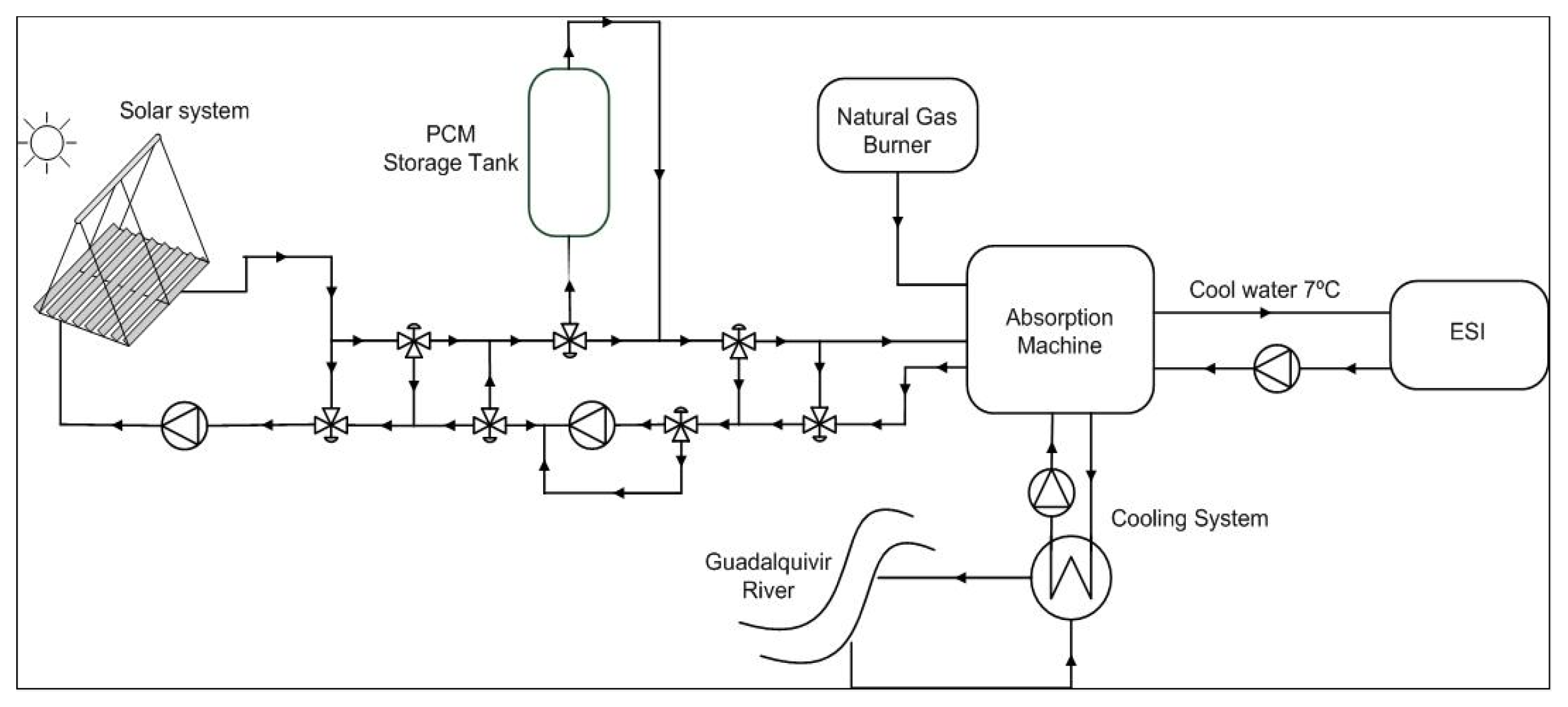
The solar cooling plant was commissioned in 2008 and consists of three subsystems: the double-effect LiBr+ water absorption chiller of 174 kW nominal cooling capacity. The solar Fresnel collector field aims at heating up the pressurized water used by the absorption machine. The PCM storage tank supplies energy to the water if there is not enough energy reaching the solar field to reach the required temperature. Figure 1 shows the scheme of the whole plant.

Water absorption chiller: this is a double-effect cycle LiBr+ absorption machine with 174 kW and a theoretical COP of 1.34, which transforms the thermal energy (hot water at 140–170 °C) coming from the Fresnel solar field or the PCM storage tank, into cold water to be used by the ESI of Seville [9]. Apart from the hot water, a cooling fluid for the condenser is needed in the absorption machine. This is obtained from the water catchment of the Guadalquivir river.

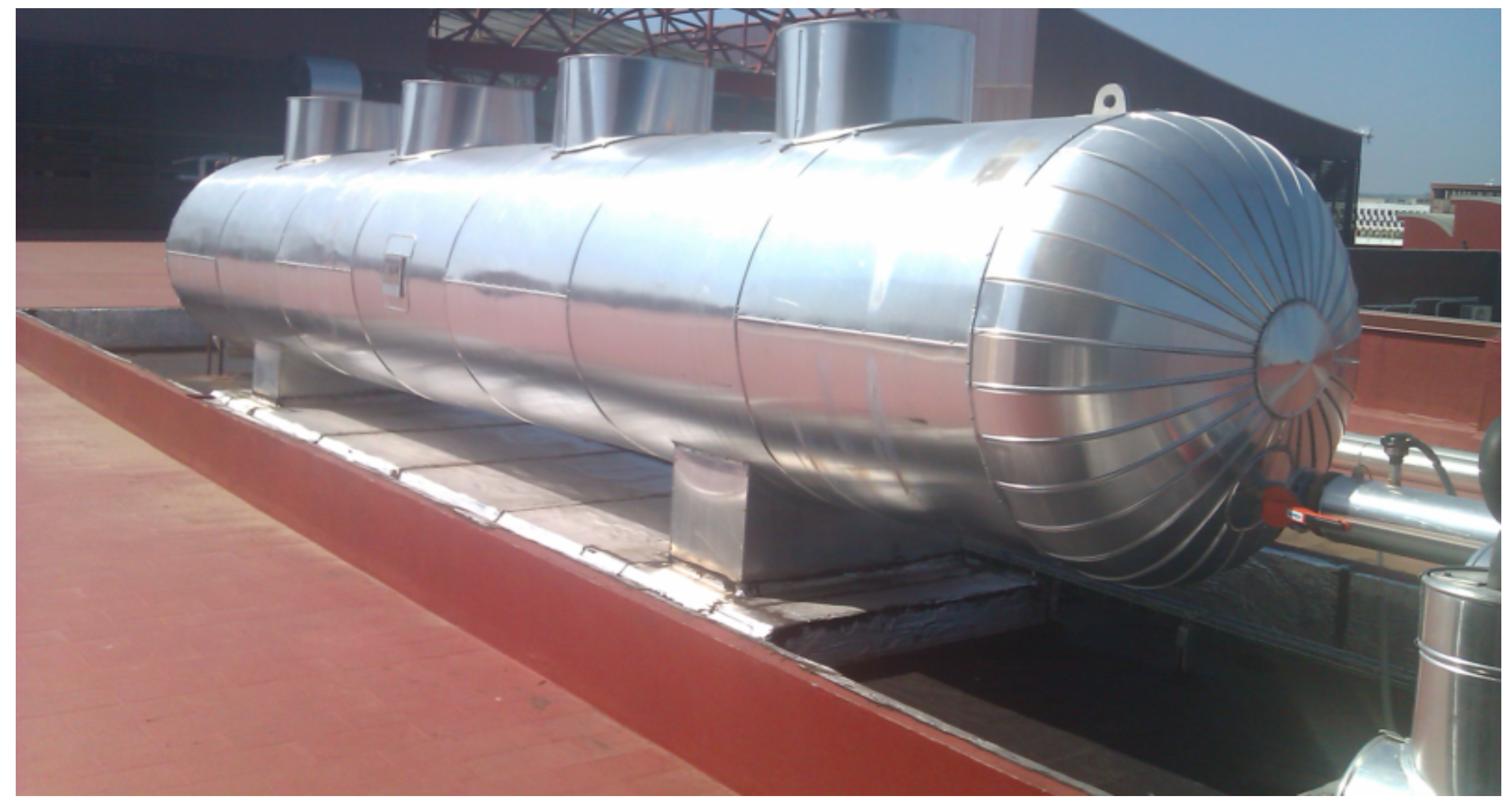
Solar field: the solar field consists of a set of Fresnel solar collectors (see Figure 2) which concentrate solar radiation onto a line where an absorption tube is located. The energy is transferred to a heat transfer fluid (in our case, pressurized water).

PCM storage tank: PCM storage is a is a shell-tube heat exchanger 18 m long and 1.31 m in diameter (Figure 3). It consists of a series of tubes containing a heat transfer fluid and PCM fills up the space between the tubes and the shell.

The storage tank uses a hydroquinone as a PCM because the melting temperature is about 170 °C, which is suitable for the water absorption chiller operational range (145–170 °C).

3. Modeling of the Plant Subsystems

In this section, the model of each subsystem comprising the whole plant is described. The solar cooling plant has four subsystems: the Fresnel solar field, the storage tank, the absorption machine and the piping system connecting them. The equations governing the dynamics of each subsystem are presented. The models are validated and compared to real data taken from the plant.

Since the main goal of these models is to be used in control algorithms, the balance equations of each subsystem should be as simple as possible and an adequate trade-off between precision and complexity is pursued.

3.1. Fresnel Solar Field

In this subsection, the mathematical model of the Fresnel collector field is presented. Two approaches are usually considered in this kind of systems: the lumped parameter model (developed in [22]) and the distributed parameter model (described in [23]). In this paper, a distributed parameter model has been used. The distributed parameter model is governed by the following two PDE equations [24,25]:

$${\rho }_m{C}_m{A}_m\frac{\partial T_m}{\partial t}=I{K}_{opt}noG-H_{l}G(T_m-T_a)-L{H}_t(T_m-T_f)$$

(1)

$${\rho }_f{C}_f{A}_f\frac{\partial T_f}{\partial t}+{\rho }_f{C}_{f}q\frac{\partial T_f}{\partial x}=L{H}_t(T_m-T_f),$$

(2)

where m subindex refers to metal and f subindex refers to a fluid. In

Table 1. Parameter description.

Symbol	Description	Units
t	Time	s
x	Space	m
$\rho$	Density	kgm${}^{-3}$
C	Specific heat capacity	JK${}^{-1}$kg${}^{-1}$
A	Cross sectional area	m${}^2$
$T(x,y)$	Temperature	K,°C
$q\left(t\right)$	Oil flow rate	m${}^3$s${}^{-1}$
$I\left(t\right)$	Solar radiation	Wm${}^{-2}$
$no$	geometric efficiency	Unitless
$K_{opt}$	Optical efficiency	Unitless
G	Collector aperture	m
$T_a\left(t\right)$	Ambient temperature	K,°C
$H_l$	Global coefficient of thermal loss	Wm${}^{-2}$°C${}^{-1}$
$H_t$	Coefficient of heat transmission metal-fluid	Wm${}^{-2}$°C${}^{-1}$
L	Length of pipe line	m

, parameters and their units are shown. The same system of equations is used to model the piping system. In this case, the radiation reaching the tube is null and the thermal losses coefficient takes a different value.

The PDE system is solved by dividing the metal and fluid in 64 segments of 1 m long. The integration step is chosen of 0.5 s.

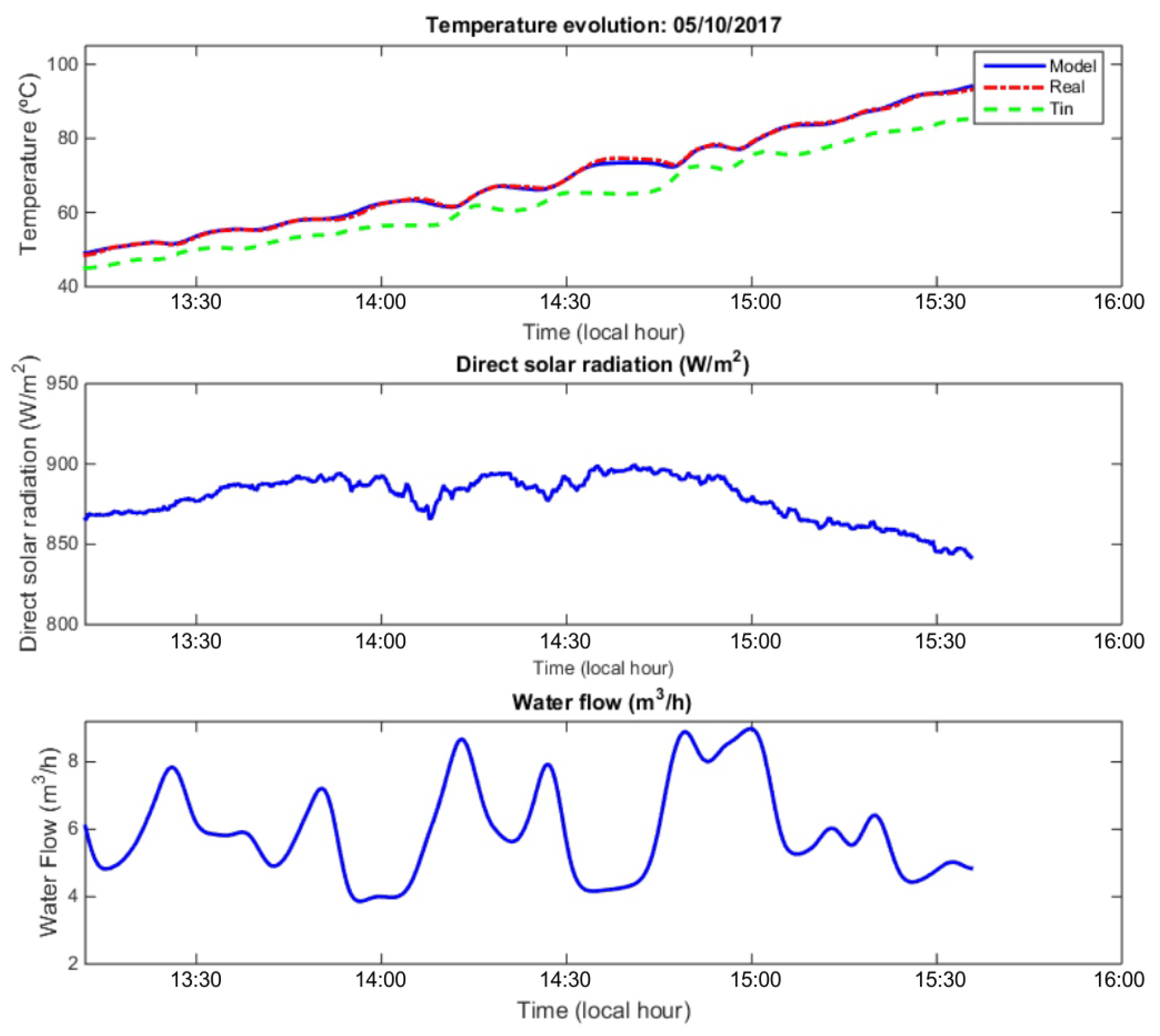
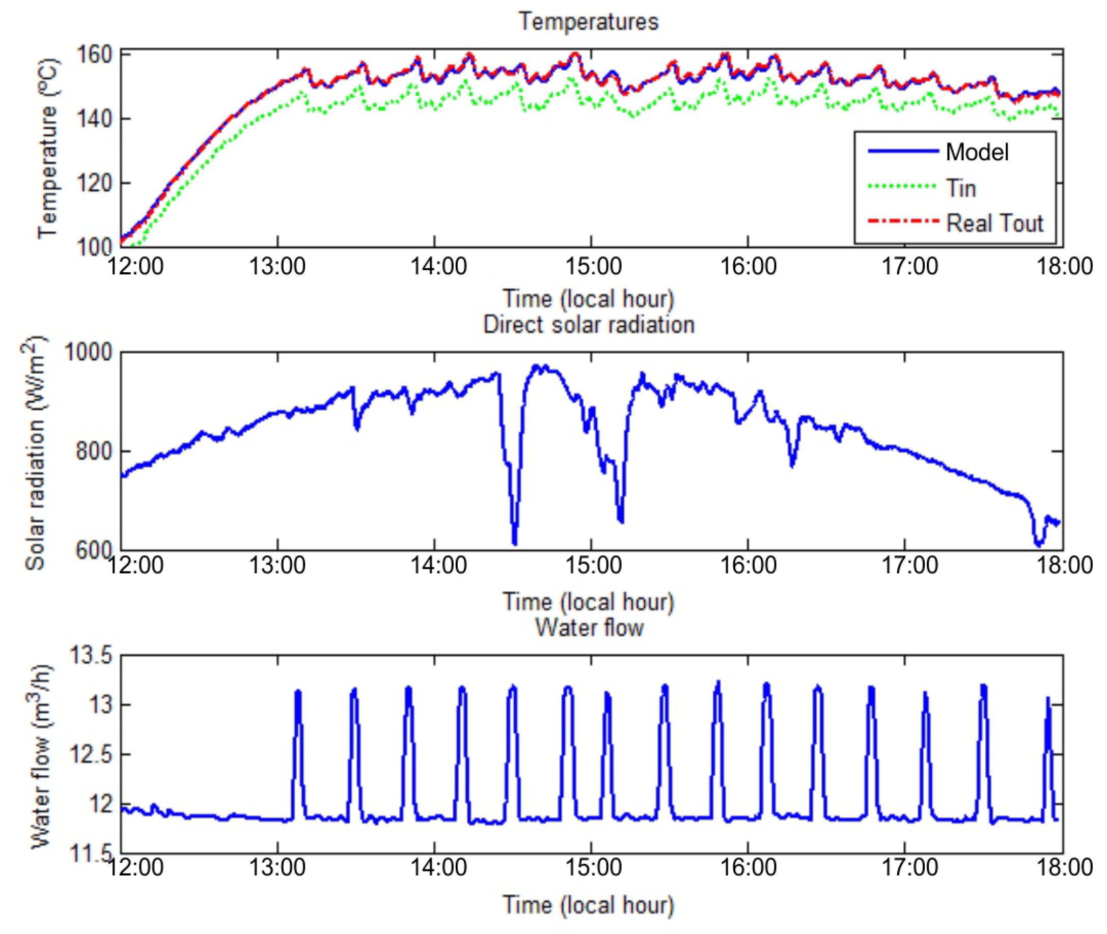
As has been mentioned before, the heat transfer fluid is pressurized water whose density and specific heat have been obtained as polynomial functions of the segment temperature using thermodynamical data of pressurized water. The heat transfer coefficient depends on the segment temperature and the water flow [26]. As far as the thermal losses coefficient is concerned, it was obtained using experimental data from the collector field [10,22]. Figure 4 and Figure 5 show a comparison between the model and the real plant evolution in two different days (in October and June). The model evolution behavior is very similar to the real solar field as can be seen.

3.2. PCM Storage Tank

In order to model the storage tank dynamics, two stages are considered: when the PCM is in the sensible heat transmission state, the PCM behavior is modeled by a double-capacity model. In the phase change stage, the solution is based on the Stephan solution. In [27], a more complete description of the PCM storage tank is carried out. The subsection provides a brief description of the model. The model was published in [28].

3.2.1. Double Capacity Model

In this stage, the model consists of two different capacitive zones, with a thermal resistance between both of them. The $r_e$ and $r_i$ radius denote exterior and interior radius respectively, $r_m$ is the separation radius between the two capacities zones, which is a parameter that has to be identified. $T_1$ and $T_2$ represent temperatures of zones 1 and 2, h is the convective heat transfer coefficient, K the conductivity, $C_p$ the specific heat and $T_{\infty }$ stands for the hot water temperature [27].

The model has two differential equations, one per zone:

Zone 1:

$$\rho C_p\pi (r_m^2-r_i^2)\frac{d{T}_1}{dt}=2h\pi r_i(T_{\infty }-T_1)-\frac{2\pi K(T_1-T_2)}{ln(r_e/ri)}.$$

(3)

Zone 2:

$$\frac{2\pi K(T_1-T_2)}{ln(r_e/ri)}=\rho C_p\pi (r_e^2-r_m)\frac{d{T}_2}{dt}.$$

(4)

The aforementioned equations are valid for the liquid and solid phase. However, parameters such as the conductivity K and the density of the hydroquinone $\rho$ may have different values.

3.2.2. Stefan Solution for Phase Change

When the PCM reaches a temperature of 170 °C, the hydroquinone reaches the melting point and the phase change stage starts. To model this stage, the liquid and solid phases are considered to be stable. The dynamics of the hydroquinone temperature is governed by the Stefan solution. This solution establishes an inferior limit of stored energy in a phase change phenomenon as well as a velocity limit for its evolution. Since the Stefan number given by the expression (5) is very small, finding a solution supposing a semi-infinite medium and that all the material is initially at the phase change temperature is possible [29,30].

$$S_T=\frac{C_p(T_f-T\left(r_i\right))}{L}.$$

(5)

The final expressions of the Stefan solution are given by Equations (6) and (7):

$$T\left(r\right)=T_f+\frac{h{r}_i}{K}\left(\frac{T_f-T_{\infty }\frac{h{r}_i}{K}ln(r_i/R)}{1-\frac{h{r}_i}{K}ln(r_i/R)}-T_{\infty }\right)ln(r/R)$$

(6)

$$\begin{array}{c}{t}_{st}=C\left(r_i\left[\frac{r_{i}h}{K}-2\right]-R^2\left(\frac{2h}{K}ln(r_i/R)+\frac{h}{K}-\frac{2}{r_i}\right)\right)\\ C={\displaystyle \frac{\rho L^{*}}{4h(T_{\infty }-T_f)}},\end{array}$$

(7)

where $R=R\left(t_{st}\right)$ is the interface position which depends on $t_{st}$ (Stefan time), $T_f$ is the melting temperature, $T\left(r\right)$ is the PCM temperature which depends on the radius and $L^{*}$ is the corrected latent heat of hydroquinone. In [27,28], all the modeling details and parameters estimation are better explained.

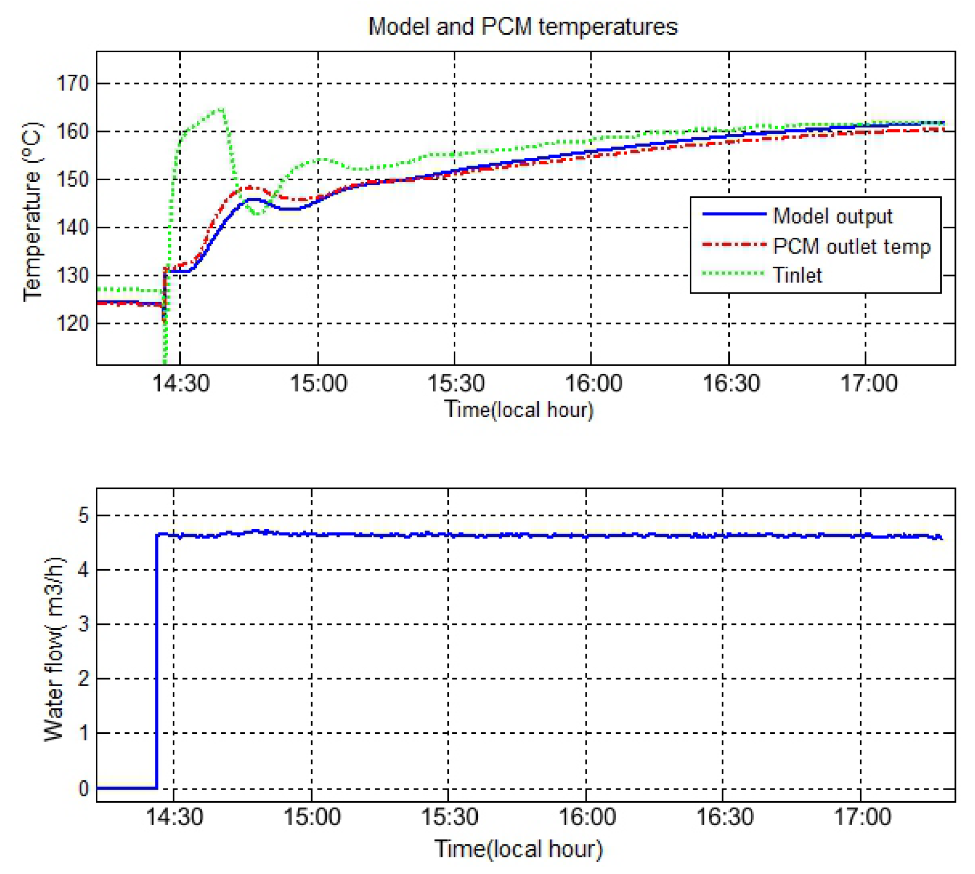
Figure 6 shows a comparison between the model and the real temperature of the storage tank evolution. At time 14.45 h the inlet valve opens and the hot water heats up the storage tank. As can be observed, the model matches well the real data with a maximum error of a $2.5\%$.

3.3. Absorption Machine Model

The water absorption chiller consists of three parts, a high temperature generator, a refrigeration system and an evaporator [31,32]. Each component is modeled as a black-box using input-output data.

More complex thermodynamical models for absorption chillers exist in literature [33], but they are too complicated to be used for control purposes. The model developed in this paper is a simplified control model.

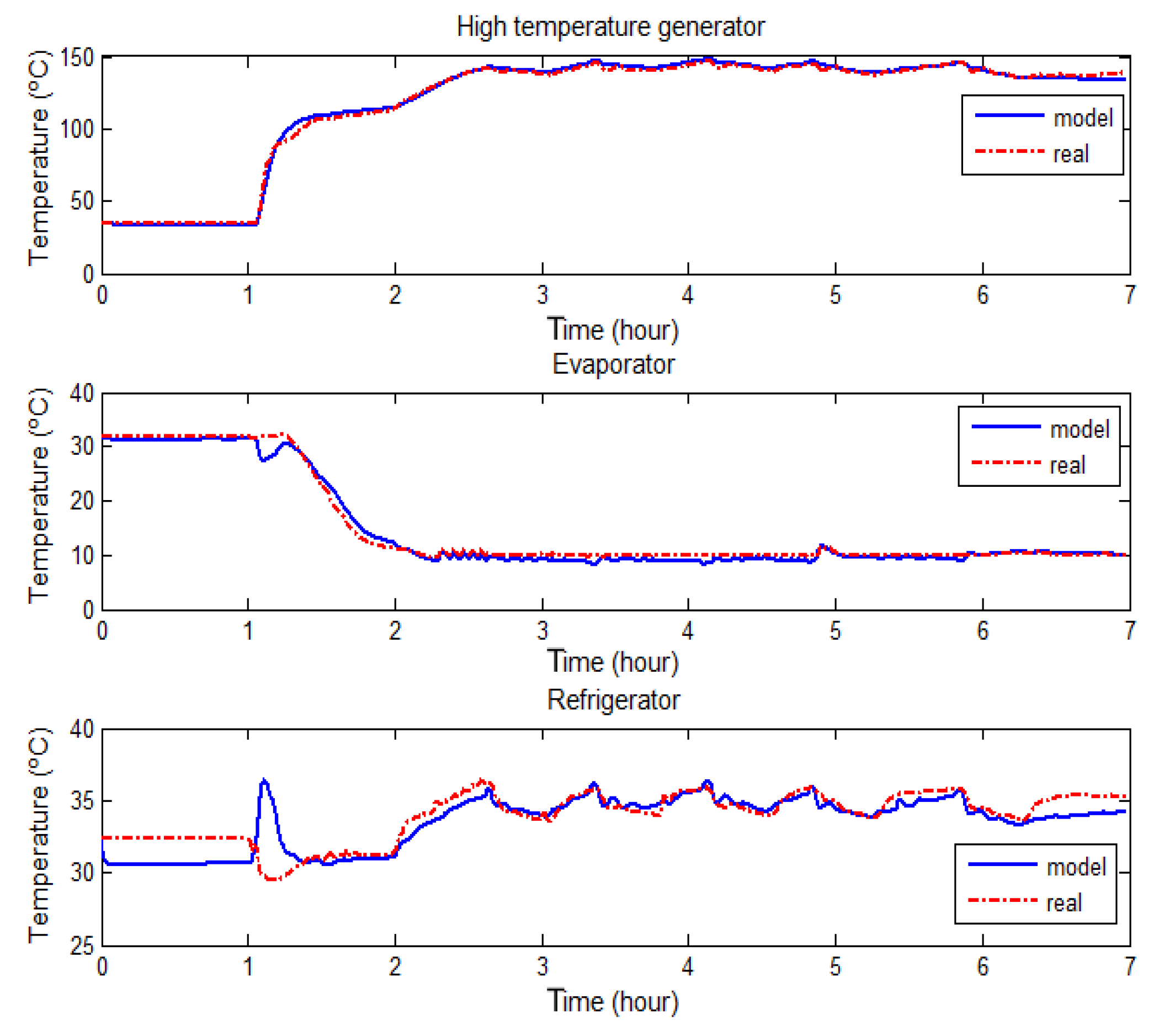
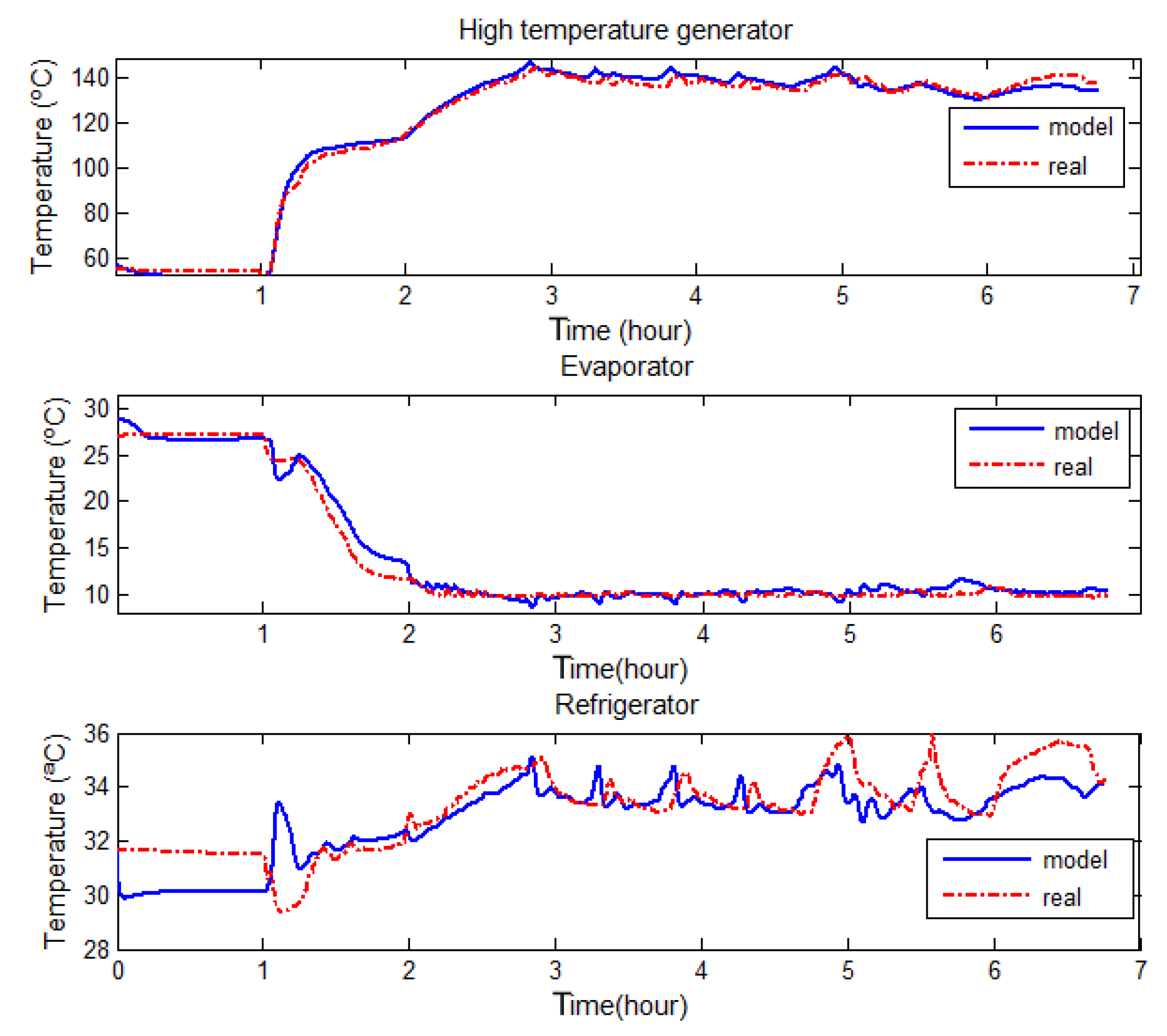
The three subsystems are described by a lumped parameter model with constant heat capacities. All the coefficients involved in the following equations were obtained using data from the real absorption machine. Figure 7 and Figure 8 show a comparison between the model and the real water chiller evolution.

3.3.1. High Temperature Generator

The energy balance equation describing the output temperature of the generator is given by Equation (8):

$$C_g\frac{d{T}_{ogen}}{dt}=Q_{cald}-Q_{gloss}+{\rho }_w{q}_h{C}_w(T_{ogen}-T_{igen}),$$

(8)

where $T_{ogen}$ and $T_{igen}$ represent the outlet and the inlet temperature of the high temperature generator, $Q_{cald}$ is the thermal power supplied by the absorption machine burner (W), $Q_{gloss}$ are the thermal losses (W), $C_g$ is the generator heat capacity, ${\rho }_w$ and $C_w$ are the density and the specific heat of the water, and $q_h$ is the generator water flow.

3.3.2. Evaporator

The energy balance equation describing the output temperature of the evaporator is given by Equation (9):

$$C_{ev}\frac{d{T}_{oevap}}{dt}=-Q_{ev}-Q_{e{v}_{l}oss}+{\rho }_w{q}_{ev}{C}_w(T_{iev}-T_{oev}),$$

(9)

where $T_{oev}$ and $T_{iev}$ represent the outlet and the inlet temperature of the evaporator, $Q_{ev}$ is the cooling power supplied by the absorption machine (W), $Q_{e{v}_{l}oss}$ are the thermal losses (W), $C_{ev}$ is the evaporator heat capacity, $q_{ev}$ is the evaporator water flow.

3.3.3. Refrigerator

The energy balance equation describing the output temperature of the refrigerator is given by Equation (10):

$$C_{refr}\frac{d{T}_{orefr}}{dt}=Q_{refr}-Q_{ref{r}_{l}oss}+{\rho }_w{q}_{ref}{C}_w(T_{irefr}-T_{orefr}),$$

(10)

where $T_{orefr}$ and $T_{irefr}$ represent the outlet and the inlet temperature of the refrigerator, $Q_{refr}$ is the thermal power dissipated by the refrigerator (W), $Q_{ref{r}_{l}oss}$ are the thermal losses (W), $C_{refr}$ is the refrigerator heat capacity, $q_{ref}$ is the refrigerator water flow.

4. Solar Field Outlet Temperature Regulator: Nonlinear Model Predictive Control Strategy

As previously mentioned in the introduction, one of the control objectives in solar plants is the regulation of the solar field outlet temperature around a desired set-point. The value of the set-point can be decided by the operator or by optimal criteria as explained in [34].

The regulation of the outlet temperature of a solar collector field around a set-point is hindered by the effect of multiple disturbance sources and its dynamics are greatly affected by the operating conditions [35]. This fact means that conventional linear control strategies do not perform well throughout the entire range of operations. In general, adaptative, robust or nonlinear schemes are needed to cope with the highly nonlinear dynamics of a solar field, especially at low flow levels. In [36] a practical nonlinear MPC is developed. In [37] a nonlinear continuous time generalized predictive control (GPC) is presented and simulation results are shown. In [38], an improvement of a gain scheduling model predictive controller is proposed and tested on a model of the ACUREX solar field.

Concerning the application of control strategies to Fresnel collector fields, there are several works in the literature. For example, in [39] a sliding model predictive control based on a feedforward compensation is developed for a Fresnel collector field and tested on a nonlinear model of a Fresnel collector field. In [10] a gain scheduling generalized predictive controller was developed and tested for a Fresnel collector field.

In this paper, a nonlinear model predictive control strategy is implemented to control the outlet temperature of the Fresnel collector field.

Model Predictive Control Strategy

An MPC control strategy consists of the following three steps [40,41]: in the first place, a model to predict the process evolution depending on a given control sequence is used. Then, it computes the control sequence by minimizing an objective function. Finally, only the first element of the computed control sequence is applied (receding horizon strategy).

The difference in MPC control strategies is usually given by the model used to predict the future evolution of the system. If linear models are used, the resulting MPC problem is a quadratic programming problem which is easily solvable and the optimum is ensured. If the model used is nonlinear, the resulting nonlinear optimization problem is computationally harder to solve and reaching the global optimum is not, in general, ensured [42].

In this paper, the model used is nonlinear. The model is a simplification of the Equation (2), considering four segments (four segments for fluid and metal temperatures) instead of 64 segments used in the full distributed parameter model. This simplification is required to alleviate the computational burden of the resulting problem although a precision loss is produced.

In general, the mathematical expression of the MPC problem can be posed as follows:

$$\underset{\Delta u}{min}J=\sum _{t=1}^{N_p}{\left(y_{k+t|k}-y_{k+t}^{ref}\right)}^{⊺}\left(y_{k+t|k}-y_{k+t}^{ref}\right)+R_u\sum _{t=0}^{N_c-1}\Delta u_{k+t|k}^{⊺}\Delta u_{k+t|k}$$

(11)

such that

$$\begin{array}{cc}\hfill y_{k+t|k}& =f(\Delta u,y_{k+t-1},y_{k+t-2},...)\hfill \\ \hfill u_{k+t|k}& =u_{k+t-1|k}+\Delta u_{k+t|k}\hfill \\ \hfill u_{min}& \le u_{k+t|k}\le u_{max}\hfill \\ \hfill t& =0,\dots ,N_p-1\hfill \end{array}$$

(12)

where $N_p$ and $N_c$ are the prediction and the control horizons respectively. The parameter $\lambda$ penalizes the control effort. Then $u_k\equiv u_{k|k}$ is applied to the system. In this case, constraints in the amplitude of the water flow and the maximum increment per iteration are considered. The sampling time of the control strategy is chosen as 20 s.

Due to the fact that only the inlet and outlet temperature are measurable, the intermediate fluid temperatures and the four metal segments temperature have to be estimated. Since the mathematical model used to predict the future evolution is nonlinear, an unscented Kalman filter is used to estimate the value of the non-measurable states.

The Kalman filter is a widely used tool for state estimation in linear systems [43]. The Kalman filter has been extended to nonlinear state estimation through algorithms such as extended Kalman filter (EFK) or unscented Kalman filter (UKF) [44]. The UKF is based on the unscented transformation, which represents a method for calculating the mean and covariance of a random variable that undergoes a nonlinear transformation [45,46]. For further information the reader is referred to [44].

5. Hybrid Model of the Solar Cooling Plant: Operation Modes

In this section the hybrid model of the solar cooling plant described in this paper, is presented.

As has been mentioned previously, the solar cooling plant can work in different operation modes. The selection of multiple operation modes will be done by a fuzzy algorithm. A particular operation mode can be defined as a particular configuration of the subsystems, valves and pumps which compose the plant (Figure 1). The choice of working in a particular operation mode is determined by the cooling demand, the state of the plant and weather conditions.

The state of the plant is described by integer (for instance, valves position) and real variables (temperatures of subsystems, water flow...). This fact leads to the need of a hybrid description of the system. In order to implement advanced control strategies, a mixed integer programming will be required if the control algorithm has to decide the operation mode [47]. Although there are efficient mixed integer programming algorithms in literature [48], they require more computational resources than those available in plant controllers. Furthermore, the complexity of solving these optimization problems increases greatly with the number of integer variables. If a high number of variables is considered, the optimization problem may be very difficult to solve in real time.

An alternative approach is selecting the operation modes by a fuzzy algorithm based on a series of membership functions obtained using data corresponding to typical operation days. The algorithm is tuned in order to fulfill two conditions: (a) the transition between modes has to be smooth, that is, fast commutations between modes are not allowed and (b) only feasible transitions between the modes are possible. Those transitions are imposed as a constraints and have been designed by the experience of the plant operators.

The operation modes are listed and briefly described below:

• Mode 0: the solar field charges the PCM storage tank. There is no cooling demand and the water chiller is off.
• Mode 1: the solar field is connected to the absorption machine through the PCM tank. This mode is useful in two situations: the storage tank can provide energy if the solar field is not able to heat the water up to the required temperature for powering the chiller. The second situation occurs when there is an excess of solar radiation: the solar field can feed the absorption machine and load the PCM tank.
• Mode 2: the PCM storage tank powers the water chiller while the solar field is heated up by recirculating water.
• Mode 3: the tank is used for heating up the piping system. It can be useful early in the morning for a quick start-up.
• Mode 4: the tank supplies hot water to the water chiller if solar collectors cannot work. For instance, in a cloudy day when solar radiation is nil and the storage tank is charged.
• Mode 5: the water chiller is powered only by the solar collectors.
• Mode 6: water is recirculated in the solar field circuit. The absorption machine uses natural gas.

Although, there are many possible transitions among the modes, only a small group of transitions are feasible. For example, supposing that the plant is working in mode 5 and a sudden decrease of radiation levels cools down the solar field temperature below the minimum required by the water chiller. In this case, if the tank has energy available, the most reasonable decision is operating in mode 1. In the next section, the transition between different operation modes is explained.

6. Transition between Operation Modes

In this section, transitions between the operation modes are described. Only modes 0–2, 5 and 6 are considered to be selected automatically by the hybrid algorithm. The initial mode is considered to be mode 6. Modes 3 and 4 are selected by the operator and deal with special cases in the plant operation. The preheating of the pipes is a operation needed before the operation starts, and it is not a possible state in a normal operation.

Not every transition among operation modes are allowed. The criterion for choosing the target operation mode is that the opening and closing of the plant valves should be smooth: including or excluding more than one subsystem in each transition is not desirable. the possible transitions are showed in

Table 2. Allowed transitions between operation modes.

	Target	M. 0	M. 1	M. 2	M. 5	M. 6
Current
M.0		X	X	$T_{0-2}$	$T_{0-5}$	$T_{0-6}$
M.1		$T_{1-0}$	X	$T_{1-2}$	$T_{1-5}$	X
M.2		$T_{2-0}$	$T_{2-1}$	X	X	$T_{2-6}$
M.5		$T_{5-0}$	$T_{5-1}$	X	X	$T_{5-6}$
M.6		$T_{6-0}$	$T_{6-1}$	X	$T_{6-5}$	X

:

The transitions depend on the plant variables: outlet temperature of the solar field, energy stored in the PCM tank, cooling demand, environmental conditions etc.

Several points are worth pointing out:

• The minimum inlet temperature allowed for correct operation is about 135 °C. This should be taken into account because thermal losses exist in the pipe connecting the solar field to the water chiller.
• The storage tank can proportionate energy for 1 h approximately when it is fully charged. The storage tank should be used only in the case when the amount of stored energy is high or the solar field is able to charge it.
• When solar radiation is high and the solar field is able to charge the storage tank and power the absorption machine, it should be done only if the temperature of the tank is high enough to ensure that the inlet temperature of the absorption machine is adequate for correct operation. For instance, if the outlet temperature of the solar field is 160 °C and the tank temperature is 120 °C, the use of mode 1 is not correct, because the temperature of the tank is smaller than that required for the absorption machine.
• The maximum absolute difference between the outlet temperature of the solar field and the storage tank temperature must be inferior to 30 °C, if the storage tank is to be used.
• In order to avoid very fast commutations of the modes, the fuzzy algorithm computes the adequate operation mode every 120 s.

The experience of operation of the plant establishes that there are conditions for some transitions, clearly defined by rules that handle limit values of variables that would be the following, presented below, where the temperature of the outlet temperature of the solar field as $T_{capt}$, the temperature of the storage tank is denoted by $T_{tank}$, the current mode is $CM$, which takes values between 0 and 6, and the cooling demand is $CD$, which takes the value of 1 if there is cooling demand and 0 if there is not. $T_{tankOUT}$ is the storage tank outlet temperature and $T_{tankMAX}=180$ °C, the storage tank maximum temperature.

Set of rules 1:

• IF $CM=6$ AND $CD=0$ AND $T_{tank}<T_{tankMAX}$ AND $6{}^{\circ }\mathrm{C}<T_{capt}-T_{tank}$ AND $T_{capt}-T_{tank}<30{}^{\circ }$C THEN select mode 0;
• IF $CM=5$ AND $CD=0$ THEN select mode 6;
• IF $CM=5$ AND $CD=1$ AND $139{}^{\circ }C<T_{capt}$ AND $T_{capt}<140{}^{\circ }$C AND $150{}^{\circ }C<T_{tank}$ AND $T_{tank}<155{}^{\circ }$C AND $T_{capt}-T_{tank}\le 30{}^{\circ }$C THEN select mode 1;
• IF $CM=5$ AND $CD=1$ AND $T_{capt}<139{}^{\circ }$C AND $165{}^{\circ }C\le T_{tank}$ THEN select mode 1;
• IF $CM=0$ AND $CD=0$ AND $T_{capt}-T_{tank}<-30{}^{\circ }$C THEN select mode 6;
• IF $CM=0$ AND $CD=0$ AND $T_{capt}-T_{tank}>30{}^{\circ }$C THEN select mode 6;
• IF $CM=0$ AND $CD=0$ AND $T_{tank}>T_{tankMAX}$ THEN select mode 6;
• IF $CM=0$ AND $CD=0$ AND $T_{capt}-T_{tank}<0{}^{\circ }$C THEN Select mode 6;
• IF $CM=0$ AND $CD=1$ AND $T_{capt}-T_{tank}<0{}^{\circ }$C THEN Select mode 6;
• IF $CM=1$ AND $CD=0$ THEN select mode 0;
• IF $CM=1$ AND $CD=1$ AND $T_{tank}<135{}^{\circ }$C THEN select mode 5;
• IF $CM=1$ AND $CD=1$ AND $-3{}^{\circ }\mathrm{C}<T_{capt}-T_{tank}<3{}^{\circ }$C THEN select mode 5;
• IF $CM=2$ AND $CD=0$ THEN select mode 0;
• IF $CM=2$ AND $CD=1$ AND $T_{tankOUT}<135{}^{\circ }$C THEN Select mode 6;

These rules work with variables whose limits are well defined. However, on the other hand, operators work with other rules that are activated with values of some variables which require a certain threshold, depending on the transition, such as:

Set of rules 2:

• IF $CM=0$ AND $CD=1$ AND $T_{capt}>140{}^{\circ }C+U_1$, THEN select mode 5;
• IF $CM=1$ AND $CD=1$ AND $T_{capt}<140{}^{\circ }C+U_1$ AND $T_{tank}<T_{tankMAX}$ AND $T_{capt}-T_{tank}<30{}^{\circ }$C OR $T_{tank}<135{}^{\circ }$C OR $|T_{capt}-T_{tank}|<3{}^{\circ }\mathrm{C}$, THEN select mode 5;
• IF $CM=6$ AND $CD=1$ AND $T_{capt}>140{}^{\circ }C+U_2$, THEN select mode 5;
• IF $CM=6$ AND $CD=1$ AND $130{}^{\circ }C<T_{capt}<140{}^{\circ }C+U_2$ AND $T_{tank}>140{}^{\circ }C+U_3$ AND $T_{capt}-T_{tank}<30{}^{\circ }$C, THEN select mode 1;
• IF $CM=5$ AND $[CD=1$ AND $T_{capt}-T_{tank}<=30{}^{\circ }$C AND $T_{capt}>140{}^{\circ }C+U_3$ AND $\left[\right[T_{tank}<T_{tankMAX}$ AND $T_{tank}<T_{capt}$ AND $T_{tank}\ge 135{}^{\circ }$C AND $|T_{capt}-T_{tank}|\ge 5]$ OR $[T_{capt}<140{}^{\circ }$C AND $T_{capt}>139{}^{\circ }$C AND $150{}^{\circ }C<T_{tank}<155{}^{\circ }C]$, THEN Select mode 1;
• IF $CM=5$ AND $CD=1$ AND $T_{capt}<139{}^{\circ }$C AND $T_{tank}>140{}^{\circ }C+U_4$ AND $T_{tank}\ge 165{}^{\circ }$CC, THEN select mode 1;
• IF $CM=5$ AND $CD=1$ AND $T_{capt}<135{}^{\circ }$C AND $T_{tank}<140{}^{\circ }C+U_4$, THEN select mode 6;
• IF $CM=0$ AND $CD=1$ AND $T_{capt}>140{}^{\circ }C+U_5$ AND $|T_{capt}-T_{tank}|>30{}^{\circ }$C, THEN select mode 1;
• IF $CM=0$ AND $CD=1$ AND $T_{capt}<135{}^{\circ }$C AND $T_{tank}>140{}^{\circ }C+U_6$, THEN select mode 2;
• IF $CM=1$ AND $CD=1$ AND $T_{capt}<135{}^{\circ }$C AND $T_{tank}<140{}^{\circ }C+U_7$, THEN select mode 0;
• IF $CM=1$ AND $CD=1$ AND $T_{capt}<135{}^{\circ }$C AND $T_{tank}>140{}^{\circ }C+U_7$, THEN Select mode 2;
• IF $CM=2$ AND $CD=1$ AND $T_{capt}>140{}^{\circ }C+U_8$ AND $T_{tank}<T_{tankMAX}$ AND $|T_{capt}-T_{tank}|$<30 ${}^{\circ }$C, THEN select mode 1;

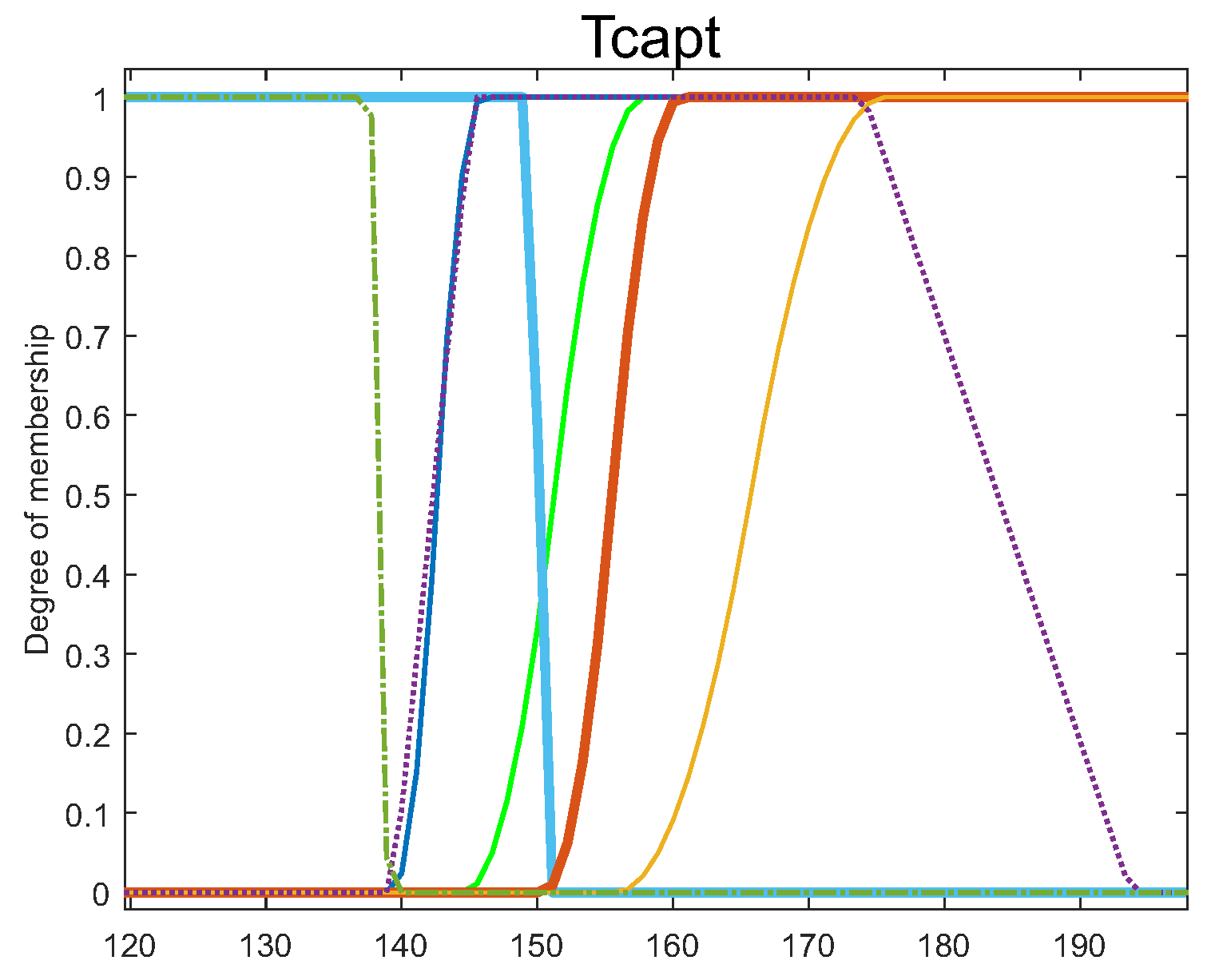
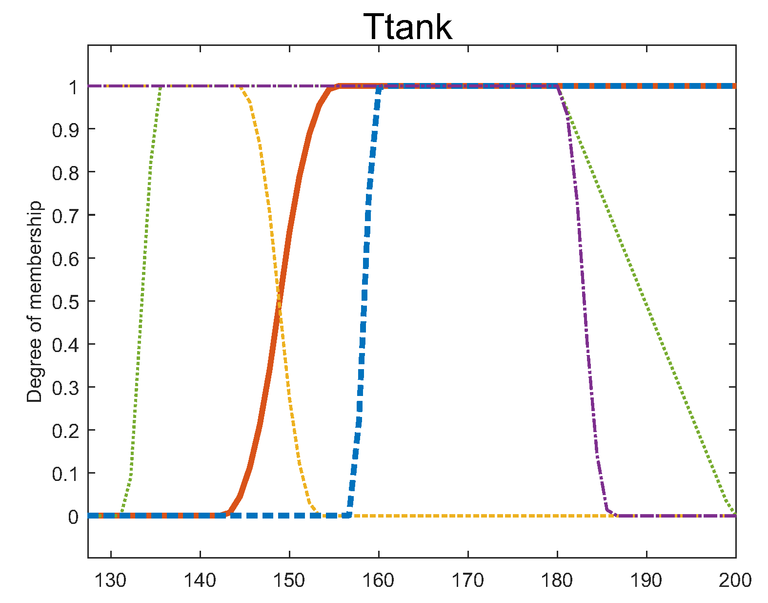
where $U_1,...,U_8$ are thresholds used by operators. A fuzzy system that integrates these last rules has been implemented. To measure the membership of any value x to the sets $x>A$ and $x<A$, spline-based S-shaped and Z-shaped membership functions have been chosen respectively:

$$S(x,a,b)=\left\{\begin{array}{cc}0& x\le a\\ 2{\left(\frac{x-a}{b-a}\right)}^2& a\le x\le \frac{a+b}{2}\\ 1-2{\left(\frac{x-b}{b-a}\right)}^2& \frac{a+b}{2}\le x\le b\\ 1& x\ge b\end{array}\right.$$

$$Z(x,a,b)=\left\{\begin{array}{cc}1& x\le a\\ 1-2{\left(\frac{x-a}{b-a}\right)}^2& a\le x\le \frac{a+b}{2}\\ 2{\left(\frac{x-b}{b-a}\right)}^2& \frac{a+b}{2}\le x\le b\\ 0& x\ge b\end{array}\right.$$

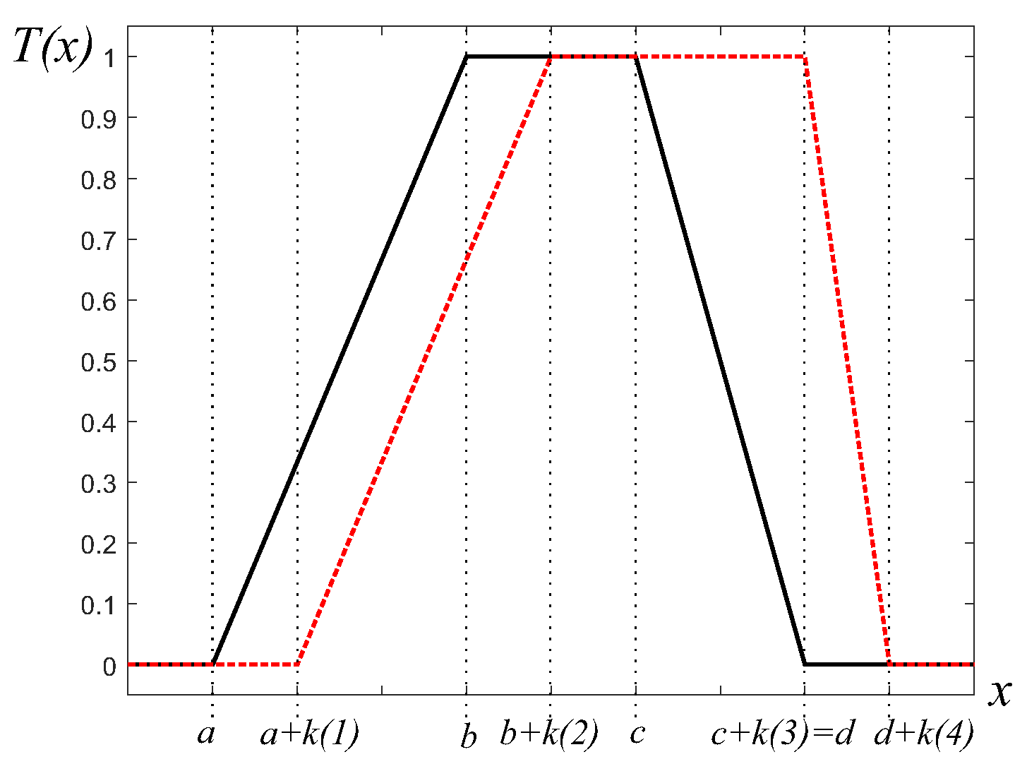
To measure the membership of the set $A<x<B$, trapezoidal membership functions $T(x,a,b,c,d)$ have been used (Figure 9):

$$T(x,a,b,c,d)=max\left(min\left(\frac{x-a}{b-a},1,\frac{d-x}{d-c}\right),0\right)$$

Membership functions have been chosen without taking into account the aforementioned thresholds and an adjustment method, based on genetic algorithms [49], has been used to position and shape the functions. A vector k has been established, whose coordinates, added to each one of the parameters of the membership functions, will give new shape and position to them. The evolutionary algorithm will find the vector k, using plant operation data for this.

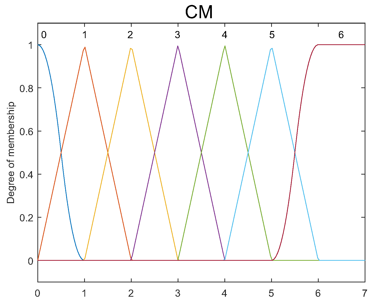
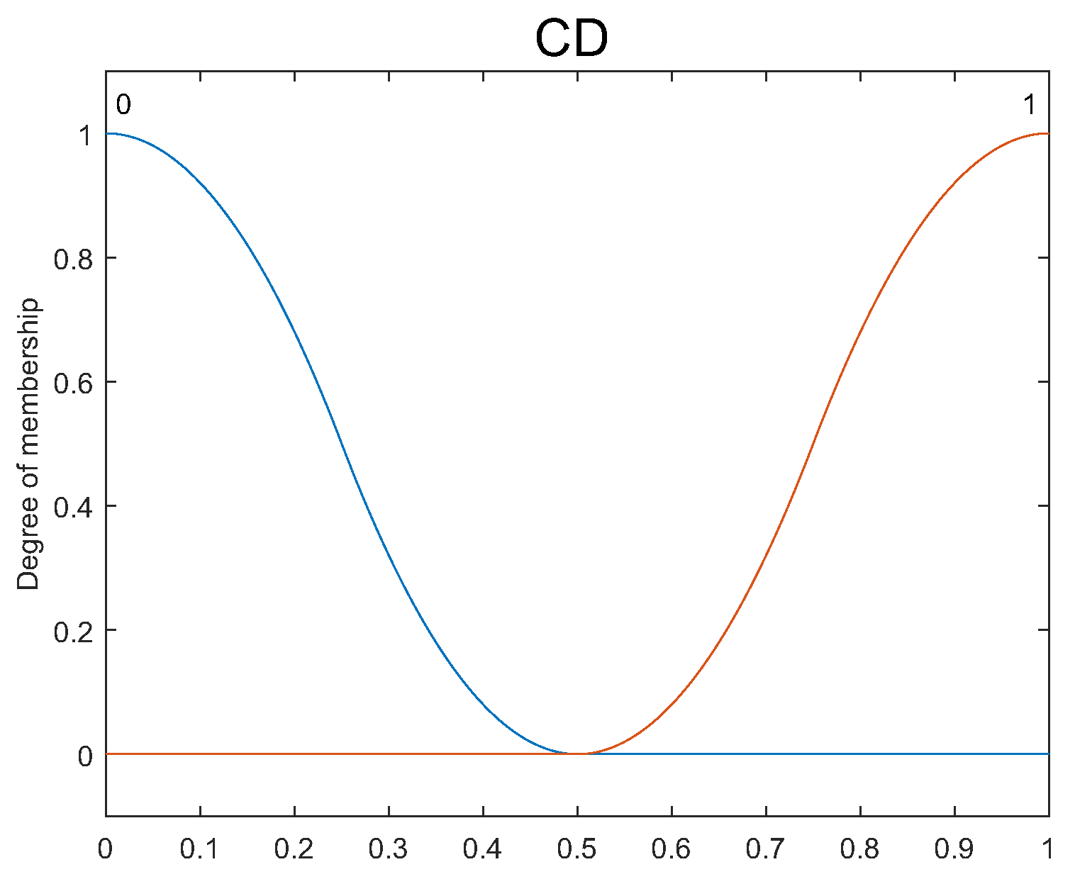
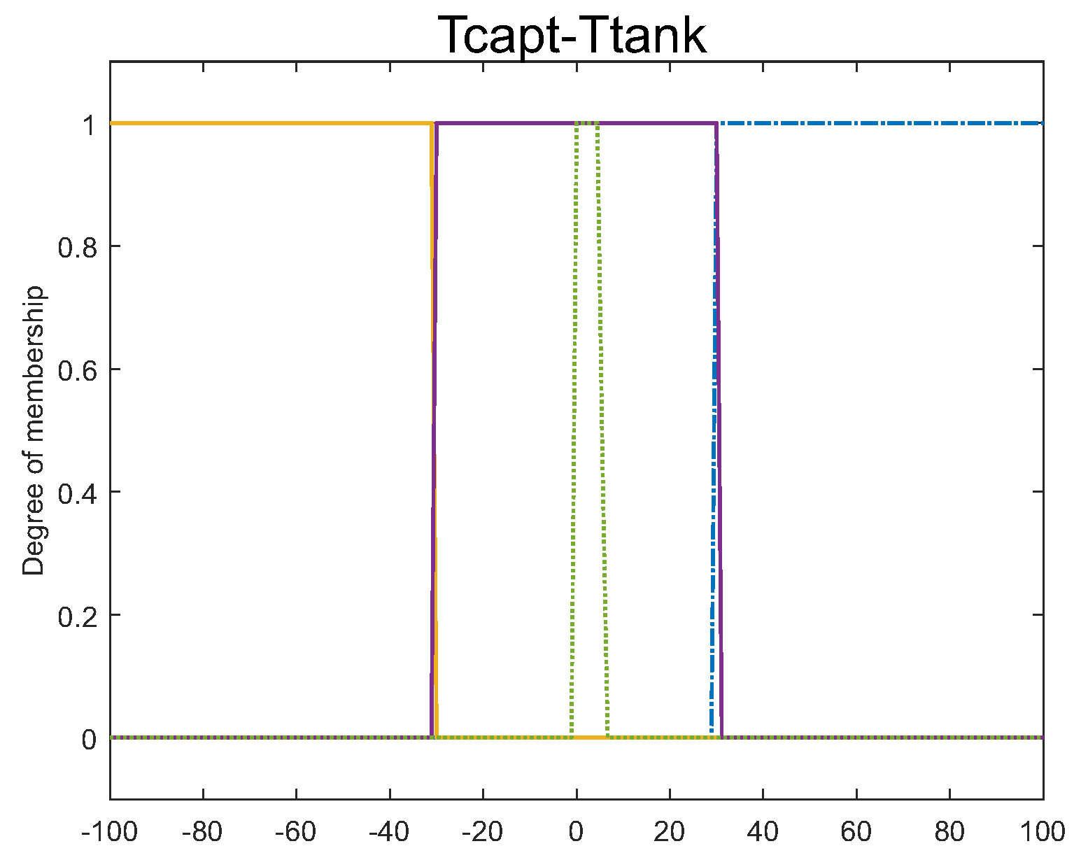
Five fuzzy inference systems (FIS) with the same antecedent structure have been designed and adjusted to evaluate whether modes 0–2, 5 and 6 are activated or not (FIS0, FIS1, FIS2, FIS5 and FIS6). The systems have five inputs: $CM$, $CD$, $T_{capt}$, $T_{tank}$ and $T_{capt}-T_{tank}$ and the membership functions, after the genetic algorithm result are shown in Figure 10, Figure 11, Figure 12, Figure 13 and Figure 14. The output variable of each FIS has one membership function with a single-valued constant (singleton membership function at 1).

The algorithm is the following (Algorithm 1)

Algorithm 1: Fuzzy algorithm

7. Simulations and Results

In this section, simulations testing the hybrid algorithm proposed in the previous section are presented. The data corresponding to solar radiation was taken from the real solar field.

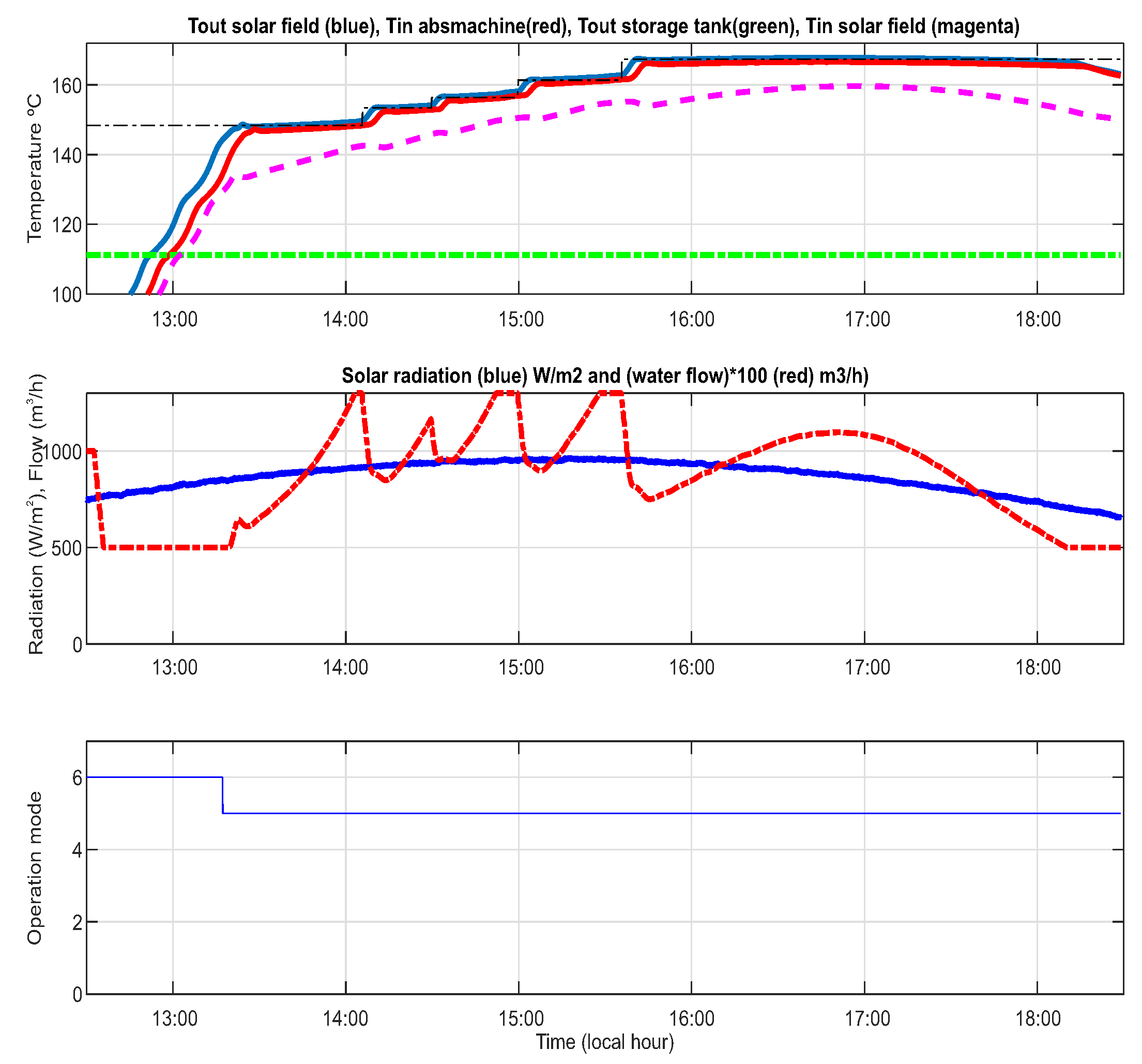
Figure 15 shows a clear day where the storage tank had a temperature about 110 °C. The initial operation mode was mode 6 in order to recirculate and heat up the water. The initial temperature reference was about 145 °C. Once the outlet temperature of the solar field reaches an adequate value to feed the absorption machine (higher than 135 °C), the fuzzy algorithm commuted to mode 5, where the solar field was able to power the absorption machine. From 14 h onwards, the temperature reference consisted of a series of increasing steps. As can be seen, the temperature regulator properly tracked these references. This was the normal operation in clear days, where the solar field was sufficient to power the water chiller.

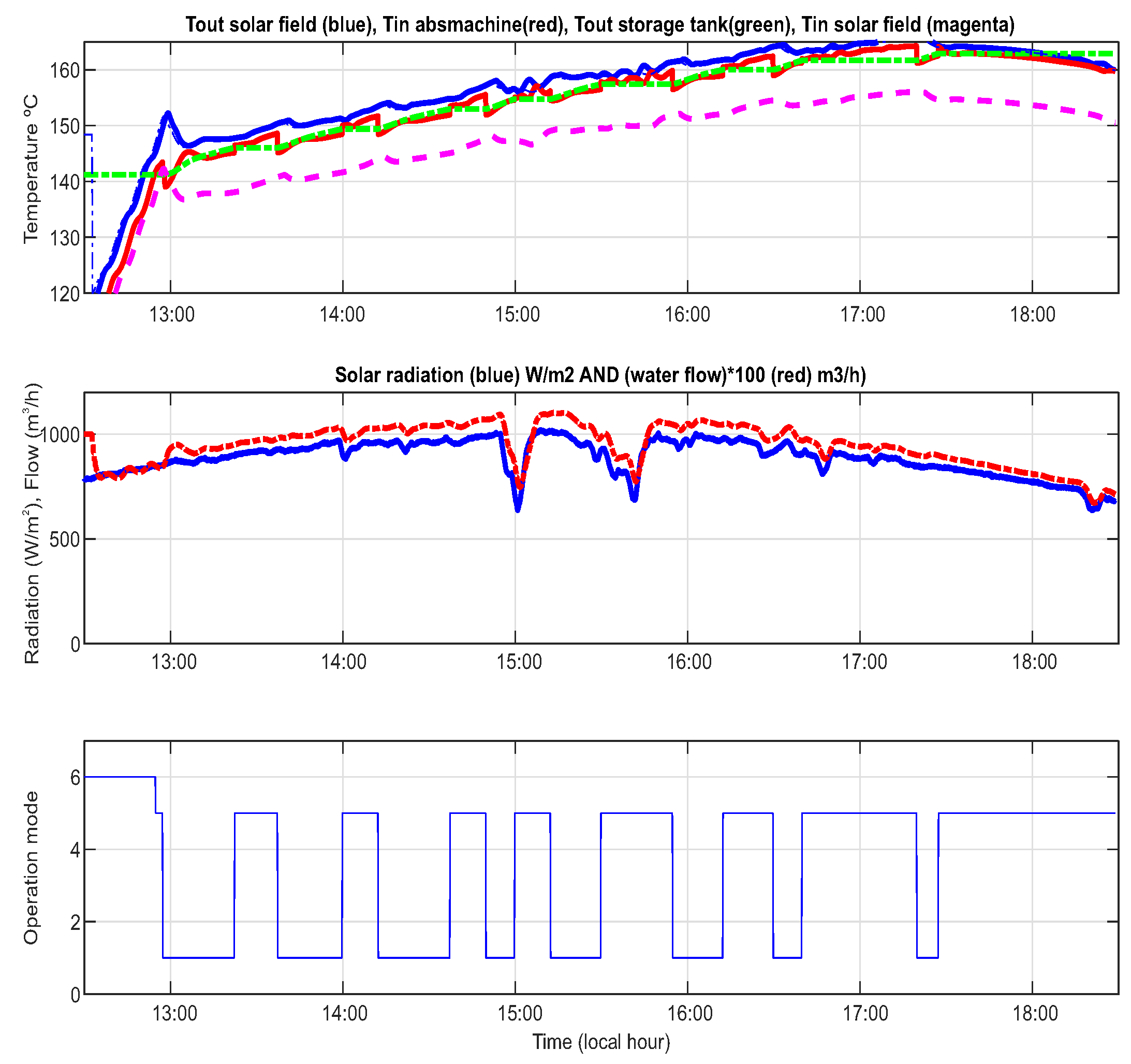
Figure 16 depicts the results of a day where some clouds affect the solar field. From 12.5 h to 12.9 h approximately, the solar field is in recirculation mode (mode 6) accumulation energy and increasing the outlet temperature. The reference temperature for the outlet temperature was 10 °C above the inlet temperature. This was done to maintain an approximately constant thermal jump without decreasing much the water flow. As can be seen, the MPC controller tracks the reference properly in spite of the radiation disturbances.

At 12.9 h the outlet temperature reached a value higher than 135 °C and the fuzzy algorithm commuted to mode 5. At 12.95 h the solar field reaches a temperature about 150 °C which makes not only powering the water chiller possible, but also accumulating energy in the storage tank. From 12.95 h onwards, the outlet temperature of the solar field was increased and the storage tank was charged (dashed green line). The fuzzy algorithm commutes between modes 5 and 1 depending on if the outlet temperature of the solar field and the storage temperature were close enough or not (approximately 4 °C). The main reason to do this was that the temperature reaching the PCM tank was about 4 °C lesser than the outlet temperature of the solar field due to the thermal losses in the pipe. Only when the outlet temperature of the solar field was higher than 4 °C than that of the storage tank, it makes sense charging it.

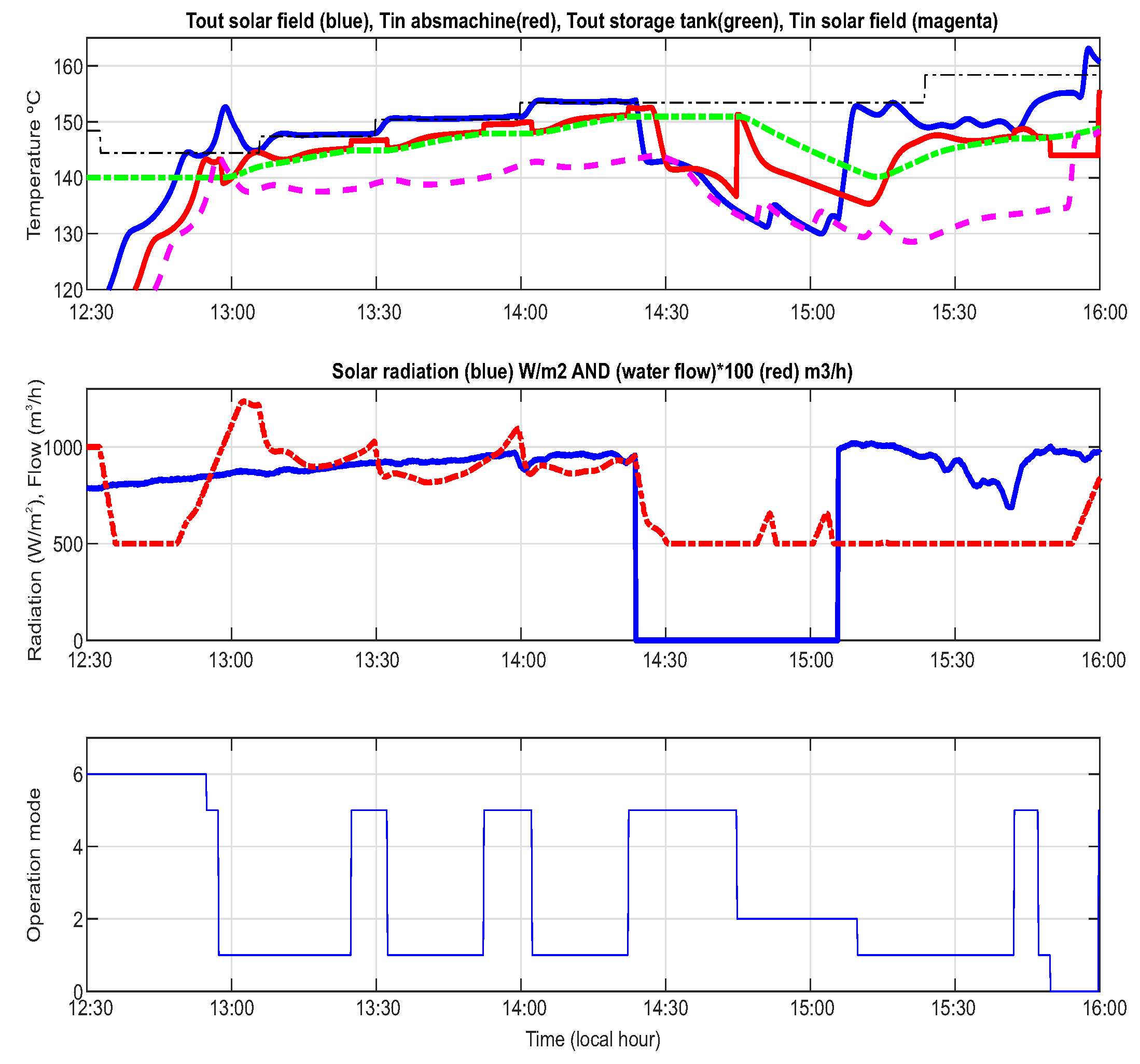
Figure 17 shows a day with scattered clouds. At the beginning of the day, the absorption machine functions burning natural gas and the operation mode was mode 6. The water recirculates through the solar collectors to be heated. At 12.9 h the water reached 145 °C and the operation mode commuted to mode 5. The solar field powered the absorption machine. At 12.95 h the mode commutes to mode 1 in order not only to power the absorption machine but to accumulate energy in the storage tank. From 13 h to 14.4 h, the temperature reference increases to accumulate more energy in the storage tank.

At 14.4 h clouds affecting the solar field appear. From 14.4 h to 14.7 h, the water flow is decreased to maintain the temperature of the solar field and the operation mode is 5 because the outlet temperature is higher than 135 °C. At 14.7 h, since there was no energy in the solar field but the storage tank possessed energy, the fuzzy algorithm commuted to mode 2: the solar field was in recirculation and the water chiller is powered by the tank only. This mode is maintained until 15.15 h, when the solar field outlet temperature increases again above 135 °C and it is capable to powers the absorption machine and charging the PCM tank. Thus, the fuzzy algorithm commutes to mode 1.

Finally, in order to test the fuzzy algorithm, from 15.8 to 16 h it was considered that no cooling demand exists. Since no cooling demand existed, the operation mode commuted to 0 and the solar field was in recirculation mode.

As can be seen, the set MPC+fuzzy algorithm has performed adequately in all the tests. This approach of using two independents algorithms has demonstrated to be very effective dealing with the operation of a hybrid system such as the solar cooling plant. The final outcome can be considered satisfactory.

8. Conclusions

Solar energy for cooling systems has been widely used to fulfill the growing air conditioning demand. The advantage of this approach is based on the fact that the need of air conditioning is usually well correlated to solar radiation.

This kind of plants can work in different operation modes resulting on a hybrid system. The control approaches designed for this kind of plant have usually a twofold goal: (a) regulating the outlet temperature of the solar collector field and (b) choose the operation mode. Since the operation mode is defined by a set of valves positions (discrete variables), the overall control problem is a nonlinear optimization problem which involves discrete and continuous variables. This problems are difficult to solve within the normal sampling times for control purposes (around 20–30 s).

A two layer control strategy is proposed in this paper. The first layer is a nonlinear model predictive controller for regulating the outlet temperature of the solar field. The second layer is a fuzzy algorithm which selects the adequate operation mode for the plant taken into account the operation conditions. The set MPC+fuzzy algorithm has performed adequately in all the tests. This approach of using two independents algorithms has demonstrated to be very effective dealing with the operation of a hybrid system such as the solar cooling plant. For the simulations, the data corresponding to solar radiation has been taken from the real solar field. Three different scenarios have been considered: clear day, clear day where some clouds affect the solar field and cloudy day. The control strategy is able to perform the normal operation in clear days, where the solar field is sufficient to power the water chiller. Where some clouds affect the solar field, the MPC controller tracks the reference properly in spite of the radiation disturbances. The system commutes between operating modes using the appropriate logic, contained in the operating rules of the fuzzy algorithm. The final outcome can be considered satisfactory.

References

- Camacho, E.F.; Berenguel, M.; Rubio, F.; Martínez, D. Control of Solar Energy Systems; Springer: London, UK, 2012. [Google Scholar]
- Camacho, E.F.; Samad, T.; Garcia-Sanz, M.; Hiskens, I. Control for Renewable Energy and Smart Grids; Technical Report; IEEE Control Systems Society: New York, NY, USA, 2011. [Google Scholar]
- Helios, I. 2018. Available online: https://solarpaces.nrel.gov/helios-i (accessed on 7 December 2019).
- Mojave Solar Project. 2018. Available online: https://solarpaces.nrel.gov/mojave-solar-project (accessed on 7 December 2019).
- Solana Generating Station. 2018. Available online: https://solarpaces.nrel.gov/solana-generating-station (accessed on 7 December 2019).
- Sonntag, C.; Ding, H.; Engell, S. Supervisory Control of a Solar Air Conditioning Plant with Hybrid Dynamics. Eur. J. Control 2008, 6, 451–463. [Google Scholar] [CrossRef]
- Kima, D.; Infante-Ferreira, C. Solar refrigeration options a state-of-the-art review. Int. J. Refrig. 2008, 31, 3–15. [Google Scholar] [CrossRef]
- Nkwetta, D.N.; Sandercock, J. A state-of-the-art review of solar air-conditioning systems. Renew. Sustain. Energy Rev. 2016, 60, 1351–1366. [Google Scholar] [CrossRef]
- Bermejo, P.; Pino, F.J.; Rosa, F. Solar absorption cooling plant in Seville. Sol. Energy 2010, 84, 1503–1512. [Google Scholar] [CrossRef]
- Gallego, A.J.; Monguio, G.; Berenguel, M.; Camacho, E.F. Gain-scheduling model predictive control of a Fresnel collector field. Control Eng. Pract. 2019, 82, 1–13. [Google Scholar] [CrossRef]
- Camacho, E.F.; Gallego, A.J.; Sánchez, A.J.; Berenguel, M. Incremental State-Space Model Predictive Control of a Fresnel Solar Collector Field. Energies 2018, 12, 3. [Google Scholar] [CrossRef]
- Zambrano, D.; Bordons, C.; Garcia-Gabin, W.; Camacho, E.F. A solar cooling plant: A benchmark for hybrid systems control. IFAC Proc. Vol. 2006, 39, 199–204. [Google Scholar] [CrossRef]
- Zambrano, D.; Bordons, C.; Garcia-Gabin, W.; Camacho, E.F. Model development and validation of a solar cooling plant. Int. J. Refrig. 2008, 31, 315–327. [Google Scholar] [CrossRef]
- Pasamontes, M.; Álvarez, J.D.; Guzmán, J.L.; Berenguel, M. Hybrid Modeling of a Solar Cooling System. IFAC Proc. Vol. 2009, 42, 26–31. [Google Scholar] [CrossRef]
- Pasamontes, M.; Álvarez, J.D.; Guzmán, J.L.; Berenguel, M.; Camacho, E.F. Hybrid modeling of a solar-thermal heating facility. Sol. Energy 2013, 97, 577–590. [Google Scholar] [CrossRef]
- Witheephanich, K.; Escano, J.M.; Gallego, A.J.; Camacho, E.F. Pressurized water temperature of a Fresnel collector field type cooling system using explicit model predictive control. In Proceedings of the IASTED Conference, Phuket, Thailand, 10–12 April 2013. [Google Scholar]
- Witheephanich, K.; Escano, J.M.; Bordóns, C. Control strategies of a solar cooling plant with Fresnel collector: A case study. In Proceedings of the 2014 International Electrical Engineering Congress (iEECON), Chonburi, Thailand, 19–21 March 2014. [Google Scholar]
- Lemos, J.M.; Neves-Silva, R.; Igreja, J.M. Adaptive Control of Solar Energy Collector Systems; Springer: Basel, Switzerland, 2014. [Google Scholar]
- Ross, T. Fuzzy Logic with Engineering Applications; John Wiley & Sons: Chichester, UK, 2004. [Google Scholar]
- Yang, Z.; Wang, Z.; Su, W.; Zhang, J. Multi-mode control method based on fuzzy selector in the four wheel steering control system. In Proceedings of the IEEE ICCA 2010, Xiamen, China, 9–11 June 2010; pp. 1221–1226. [Google Scholar] [CrossRef]
- Huchang, L.; Xungie, G.; Zeshui, X. A survey on decision making theory and methodologies of hesitant fuzzy linguistic term set. Syst. Eng.-Theory Pract. 2017, 37, 35–48. [Google Scholar]
- Robledo, M.; Escano, J.M.; Núnez, A.; Bordons, C.; Camacho, E.F. Development and Experimental Validation of a Dynamic Model for a Fresnel Solar Collector. IFAC Proc. Vol. 2011, 44, 483–488. [Google Scholar] [CrossRef] [Green Version]
- Spoladore, M.; Camacho, E.F.; Valcher, M.E. Distributed Parameters Dynamic Model of a Solar Fresnel Collector Field. IFAC Proc. Vol. 2011, 44, 14784–14790. [Google Scholar] [CrossRef]
- Camacho, E.F.; Rubio, F.R.; Berenguel, M. Advanced Control of Solar Plants; Springer: London, UK, 1997. [Google Scholar]
- Gallego, A.J.; Camacho, E.F. Estimation of effective solar radiation in a parabolic trough field. Sol. Energy 2012, 86, 3512–3518. [Google Scholar] [CrossRef]
- Kreith, F.; Manglik, R.M.; Bohn, M.S. Principles of Heat Transfer, 7th ed.; Cengage Learning: Boston, MA, USA, 2011. [Google Scholar]
- Ruíz-Pardo, A.; Salmerón, J.M.; Cerezuela-Parish, A.; Gil, A.; Álvarez, S.; Cabeza, L.F. Numerical simulation of a thermal energy storage system with PCM in a shell and tube tank. In Proceedings of the 12th International Conference on Energy Storage (InnoStock 2012), Lleida, Spain, 16–18 May 2012. [Google Scholar]
- Gallego, A.J.; Ruíz-Pardo, A.; Martín-Macareno, C.; Cabeza, L.F.; Camacho, E.F.; Oró, E. Mathematical modeling of a PCM storage tank in a solar cooling plant. Sol. Energy 2013, 93, 1–10. [Google Scholar] [CrossRef]
- Lunardini, V.J. Heat Transfer in Cold Climates; Van Nostrand Reinhold Company: New York, NY, USA, June 1981. [Google Scholar]
- Naterer, G.F. Heat Transfer in Single and Multiphase Systems; CRC Press: Boca Raton, FL, USA, 2002; ISBN 978-0-8493-1032-4. [Google Scholar]
- Prasartkaew, B. Mathematical Modeling of an Absorption Chiller System Energized by a Hybrid Thermal System: Model Validation. Energy Procedia 2013, 34, 159–172. [Google Scholar] [CrossRef] [Green Version]
- Karimi, M.N.; Ahmad, A.; Aman, S.; Jamshed-Khan, M.D. A review paper on Vapor absorption system working on LiBr/H2O. Int. Res. J. Eng. Technol. 2018, 5, 857–864. [Google Scholar]
- Grossman, G.; Wilk, M. Advanced modular simulation of absorption systems. Int. J. Refrig. 1994, 17, 231–244. [Google Scholar] [CrossRef]
- Camacho, E.F.; Gallego, A.J. Optimal Operation in Solar Trough Plants: A case study. Sol. Energy 2013, 95, 106–117. [Google Scholar] [CrossRef]
- Pin, G.; Falchetta, M.; Fenu, G. Adaptative time-warped control of molten salt distributed collector solar fields. Control Eng. Pract. 2007, 16, 813–823. [Google Scholar] [CrossRef]
- Andrade, G.A.; Pagano, D.J.; Álvarez, J.D.; Berenguel, M. A practical NMPC with robustness of stability applied to distributed solar power plants. Sol. Energy 2013, 92, 106–122. [Google Scholar] [CrossRef]
- Khoukhi, B.; Tadjine, M.; Boucherit, M.S. Nonlinear continuous-time generalized predictive control of solar power plant. Int. J. Simul. Multidiscip. Design Optim. 2015, A3, 1–12. [Google Scholar] [CrossRef]
- Alsharkawi, A.; Rossiter, J.A. Towards an improved gain scheduling predictive control strategy for a solar thermal power plant. IET Control Theory Appl. 2017, 11, 1938–1947. [Google Scholar] [CrossRef] [Green Version]
- Lu, X.-J.; Dong, H.-Y. Application Research of Sliding Mode Predictive Control Based on Feedforward Compensation in Solar Thermal Power Generation Heat Collecting System. Int. J. Hybrid Inf. Technol. 2016, 9, 211–220. [Google Scholar]
- Camacho, E.F.; Bordons, C. Model Predictive Control, 2nd ed.; Springer: London, UK, 2004. [Google Scholar]
- Rawlings, J.; Mayne, D. Model Predictive Control: Theory and Design; Nob Hill Publishing, LLC: Madison, WI, USA, 2009. [Google Scholar]
- Findeisen, R.; Allgöwer, F. An Introduction to Nonlinear Model Predictive Control; Technical Report; Institute for Systems Theory in Engineering, University of Stuttgart: Stuttgart, Germany, 2006. [Google Scholar]
- Kalman, R. A new approach to linear filtering and predictions problem. Trans. ASME J. Basic Eng. 1960, 82, 35–60. [Google Scholar] [CrossRef]
- Haykin, S. Kalman Filtering and Neural Networks; A Wiley-Interscience Publication: New York, NY, USA, 2001. [Google Scholar]
- Romanenko, A.; Castro, J.A. The unscented Kalman filter as an alternative to the EKF for nonlinear state estimation: A simulation case study. Comput. Chem. Eng. 2004, 28, 347–355. [Google Scholar] [CrossRef]
- Wang, Y.; Qiu, Z.; Qu, X. An Improved Unscented Kalman Filter for Discrete Nonlinear Systems with Random Parameters. Discret. Dyn. Nat. Soc. 2017, 2017, 1–10. [Google Scholar] [CrossRef]
- Zambrano, D. Modelado y Control Predictivo Híbrido de una Planta de Refrigeración Solar. Ph.D. Thesis, Escuela Superior de Ingenieros de Sevilla, Sevilla, Spain, 2007. [Google Scholar]
- Bertsekas, D.P. Convex Analisys and Optimization, 1st ed.; Athena Scientific: Nashua, NH, USA, April 2003. [Google Scholar]
- Goldberg, D.E. Genetic Algorithms in Search, Optimization, and Machine Learning; Addison-Wesley: New York, NY, USA, 1989. [Google Scholar]
Figure 1.
Plant general scheme.
Figure 2.
Fresnel collector field.
Figure 3.
Phase change material (PCM) storage tank.
Figure 4.
Solar field evolution model vs. real: 5 October 2017.
Figure 5.
Solar field evolution model vs. real: 29 June 2009.
Figure 6.
PCM temperature evolution: model vs. real.
Figure 7.
Absorption machine model vs. real: 19 July 2010.
Figure 8.
Absorption machine model vs. real: 21 July 2010.
Figure 9.
Trapezoidal membership function adjustment.
Figure 10.
Inputs memberships functions of variable current mode (CM).
Figure 11.
Inputs memberships functions of variable cooling demand (CD).
Figure 12.
Inputs memberships functions of variable .
Figure 13.
Figure 14.
Figure 15.
Operation modes in a clear day.
Figure 16.
Operation modes in a clear day: storage tank charging.
Figure 17.
Operation modes in a cloudy day.