Life Cycle Cost of Building Energy Renovation Measures, Considering Future Energy Production Scenarios


1
Energy Technology, Dalarna University, 791 88 Falun, Sweden
2
Business, Society and Engineering, Mälardalen University, 721 23 Västerås, Sweden
3
Environmental Technology and Management, Linköping University, 581 83 Linköping, Sweden
*
Author to whom correspondence should be addressed.
Energies 2019, 12(14), 2719; https://doi.org/10.3390/en12142719
Submission received: 11 June 2019
/
Revised: 3 July 2019
/
Accepted: 12 July 2019
/
Published: 16 July 2019
(This article belongs to the Special Issue Select papers from International Conference on Renewable Energy—ICREN 2019)
Abstract
:A common way of calculating the life cycle cost (LCC) of building renovation measures is to approach it from the building side, where the energy system is considered by calculating the savings in the form of less bought energy. In this study a wider perspective is introduced. The LCC for three different energy renovation measures, mechanical ventilation with heat recovery and two different heat pump systems, are compared to a reference case, a building connected to the district heating system. The energy system supplying the building is assumed to be 100% renewable, where eight different future scenarios are considered. The LCC is calculated as the total cost for the renovation measures and the energy systems. All renovation measures result in a lower district heating demand, at the expense of an increased electricity demand. All renovation measures also result in an increased LCC, compared to the reference building. When aiming for a transformation towards a 100% renewable system in the future, this study shows the importance of having a system perspective, and also taking possible future production scenarios into consideration when evaluating building renovation measures that are carried out today, but will last for several years, in which the energy production system, hopefully, will change.
1. Introduction
The European Union (EU) directive regarding the energy performance of buildings states that each member state should ensure that all new buildings built from the end of 2020 should be nearly zero energy buildings [1]. Each member state sets its own definition of a nearly zero energy building. In Sweden, the requirements for a nearly zero energy building involve a so-called primary energy number, which is expressed as the amount of primary energy used per year and the building area [2]. The calculation is based on the yearly final energy demand, where different energy carriers such as electricity and district heating (DH) are weighted using primary energy factors.
DH is the main energy carrier to multi-family buildings in Sweden, accounting for 90% of the final energy used for heating and hot water in 2016 [3]. Counting all dwellings and non-residential premises, DH supplied almost 60% of the final energy used for heating and hot water in 2016. The second largest part is supplied by electricity-based heating, e.g., heat pumps (HPs) and mechanical ventilation with heat recovery (MVHR). As HPs utilize heat sources such as the outdoor air or geothermal energy, the delivered useful heat will be higher than the amount of purchased energy (often electricity). This means that it is easier to fulfill any energy demand requirements for HPs than for DH, when the focus is on final energy.
Gustafsson et al. [4] conclude that the current requirements for nearly zero energy buildings in Sweden favor HPs. There are, however, several studies, including Gustafsson et al., which show that DH has lower carbon dioxide emissions than HPs when global emissions from marginal electricity production are included [4,5]. Compared to DH, MVHR also reduces the final energy demand, at the expense of an increased electricity demand. Even though both HPs and MVHR reduce the final energy demand, the changes in carbon dioxide emissions are not linear. This is demonstrated by Lidberg et al. [6], where both HPs and MVHR are evaluated compared to DH. Even though the HP case results in the lowest final energy use, the MVHR case had the lowest carbon dioxide emissions. This is the result when the impact upon the local DH system is included in the analysis. Another way to expand the system boundaries beyond final energy is to do a life cycle assessment, where the impact from the building process and materials are included as well. This has been done by Ramírez-Villegas et al. [7], where different building renovation measures (including MVHR) have been studied on an existing building connected to the DH system. Studies have shown that the environmental impact differs considerably, depending on the system boundary used, and also upon different energy system scenarios [6,8].
Hence, the environmental impact from different building energy renovation measures is ambiguous, and depends both on local conditions and uncertain future developments in the energy system, as well as upon system boundaries. Another important decision parameter is whether the measures are economical or not. One common method for evaluating the economical aspect is life cycle cost (LCC) assessment, where the whole lifetime of the measure is taken into consideration. LCC assessment is usually carried out from a building perspective, where the energy system cost is included in the energy price for the different energy carriers. This is done for different energy renovation measures by Gustafsson et al. and Paiho et al. [9,10]. They both show that from a building perspective, the LCC is lower for the HP cases, compared to DH. This is, however, based on today’s energy system and energy prices. The energy system cost is also simplified using the customer price for electricity and DH. As well as expanding the system boundary to include the whole life cycle, the system boundary should be expanded in order to include any costs for the whole energy system.
In Sweden, 75% of the dwellings in multi-family buildings were built before 1980 [11]. The largest construction boom occurred between 1965 and 1975, due to a big housing program to cope with the increasing population [12]. Houses built within this period are currently in need of renovation, if they have not been renovated already. Energy renovations in order to reach energy efficiency goals are usually included as well, and not just renovations carried out in order to maintain functionality. It is easier, as mentioned above, to reach energy goals set in terms of final energy, using HPs or MVHR instead of DH. Converting from DH to HP or MVHR is therefore often done in these cases.
In this study, the LCC for different energy renovation measures in a multi-family building are calculated, including production, operation and maintenance costs for the energy system. In addition to expanding the system boundary, future 100% renewable scenarios are analyzed instead of the current system. The building used is a typical Swedish multi-family building from the 1965–1975 housing program, with DH and mechanical exhaust ventilation as a reference system. Three energy renovation measures in the form of HP and MVHR solutions are then compared to the reference case, evaluating the economic effects on the energy system.
2. Methods
The life cycle cost (LCC) is calculated for different energy renovation measures in a multi-family building for a variety of future energy system scenarios. The savings in the form of less bought energy due to a lower demand after the renovation measures is calculated as the change in energy system cost for the different energy system scenarios. Figure 1 shows an illustration of the methodology used. A reference building is simulated in order to get hourly values of the energy demand. The hourly energy demand is used to calculate the energy system cost for eight future energy system scenarios. Three energy renovation measures are also simulated, and the energy system costs are calculated for the eight energy system scenarios for each energy renovation measure.
The cost for the energy renovation measures are calculated, and the total LCC is achieved by adding the energy system savings. Details regarding the LCC calculation, the building simulation and the energy system scenarios are found in Section 2.1, Section 2.2 and Section 2.3.
2.1. Life Cycle Cost Calculation
The LCC calculations done in this study comply with conventional LCC methodology and the standards for the LCC of buildings [13,14], with the important difference that the calculated costs consider the whole energy system, rather than just the building. The LCC is calculated from a socio-economic perspective, which means that no taxes, subsidies etc., are included. An exchange rate of 10.5 for EUR to SEK has been used for costs in Swedish kronor (SEK) found in some references. The LCC is calculated over the lifetime of the system, but since several units are included with different lifetimes, a project lifetime is set to 30 years. Reinvestment is needed when the technical lifetime of specific equipment is less than the project lifetime. A linear depreciation is assumed in order to calculate the residual value for equipment with a longer technical lifetime than the project lifetime.
The total LCC for the energy renovation measures is calculated as the cost for the measures themselves, together with the cost for the surrounding energy system. For both the renovation measures and the energy system, the LCC includes the capital cost, annual operation and maintenance (O&M) costs, the reinvestment cost and the residual value, according to Equation (1).
where ICC is the initial capital cost, A is the annual O&M cost, R is the reinvestment cost, and Res is the residual value. Costs for disposal of expired assets are assumed to be negligible, and are not included. The costs used in the calculations are listed in Appendix A, Table A1 and Table A2.
LCC = ICC + A + R − Res,
2.2. Building Renovation Measures
The building model used in the simulations represents a Swedish 1960s four-story multi-family building, with a heated floor area of 4700 m2 and 60 apartments. The same model was previously used by Gustafsson et al. [9] and Swing Gustafsson et al. [17] In the reference case, the building has an annual space heating demand of 114 kWh/m2·y and a domestic hot water demand of 25 kWh/m2·y, covered by DH, and an electricity use for ventilation and pumps of 4.4 kWh/m2·y.
The ventilation rate is set to 0.5 h−1, complying with Swedish building standards [2] out of which 0.4 h−1 is assumed be controlled air flows through ventilation ducts and the remaining 0.1 h−1 is modeled as infiltration through the building envelope.
In the reference case, the building is assumed to have mechanical exhaust ventilation and DH. This system is considered representative for the studied building type and its period of construction, as 68% of the Swedish multi-family buildings built in the 1960s and 70s have mechanical exhaust ventilation [18], and about 90% of all Swedish multi-family buildings have DH [3]. The studied renovation measures consist of three other heating and ventilation systems, denoted A, B and C. In system A, the ventilation system is changed to mechanical ventilation with heat recovery (MVHR). In systems B and C, an exhaust air heat pump (EAHP) [19] is installed in addition to the DH. The EAHP is used only for heating in system B, and for both heating and domestic hot water in system C. A summary of the heating and ventilation systems is found in Table 1.
Simulations of the building with the different renovation measures were done in TRNSYS 17 [20] with Meteonorm climate data [21] for Stockholm (Bromma Airport). The output from the simulations, in form of hourly DH and electricity demand, were used as an input for the energy system cost calculation.
Regarding the heating and ventilation systems, all systems concerning the ventilation system are included in the building cost. The cost for the DH substation is however included in the energy system cost. The costs and lifetimes used in the calculations are listed in Appendix A, Table A1. The investment costs described in the table include both the capital cost and labor cost, where the latter is taken from statistics [22]. O&M costs are taken to be 1% of the initial investment costs.
2.3. Energy System Scenarios
The energy system consists of both the DH system and the electricity system delivering energy to the building. Costs for both the production and distribution are considered. The DH distribution includes the cost for the pipes and the substation in the building, as well as the distribution losses. The DH production is dimensioned based on the heat demand profile of the building and the distribution losses. The base load in the DH system is assumed to be covered by combined heat and power (CHP), with heat only boilers (HOB) as peak boilers. Two different CHP dimensions are considered in the different energy system scenarios. Two different fuels are also considered in the different scenarios. The peak production unit is assumed to be a biomass-based HOB in all scenarios.
The electricity production units are dimensioned to cover the building’s electricity demand, including distribution losses, after the electricity production from the CHP unit is credited. In the electricity system, wind power is dimensioned to cover the annual electricity demand. Two different kinds of electrical backup power are considered in the different scenarios. The electricity distribution costs taken into consideration are the distribution losses, as well as the need for additional investments due to a large share of intermittent power production.
This results in a total of eight different scenarios, which are shown in Figure 2. The energy system calculation is based on the method by Swing Gustafsson et al. [23], but with changes in order to adapt to a multi-family building. The following subsections, Section 2.3.1, Section 2.3.2, Section 2.3.3 and Section 2.3.4., describe all assumptions and costs in detail. The costs and lifetimes used in the calculations are listed in Appendix A, Table A2.
2.3.1. District Heating Distribution
The DH is assumed to be a medium temperature DH, the same temperature levels as most of the DH networks in Sweden, also called 3rd generation DH. The substation, investment cost for the pipes and the yearly O&M costs are included in the DH distribution costs. All pipe and substation costs are based on the urban conditions and experiences in Denmark and Sweden [24]. The dimensions of the substation and pipes are based on the buildings’ heat demand. The total distribution losses are assumed to be 10%, according to Danish and Swedish experience [24].
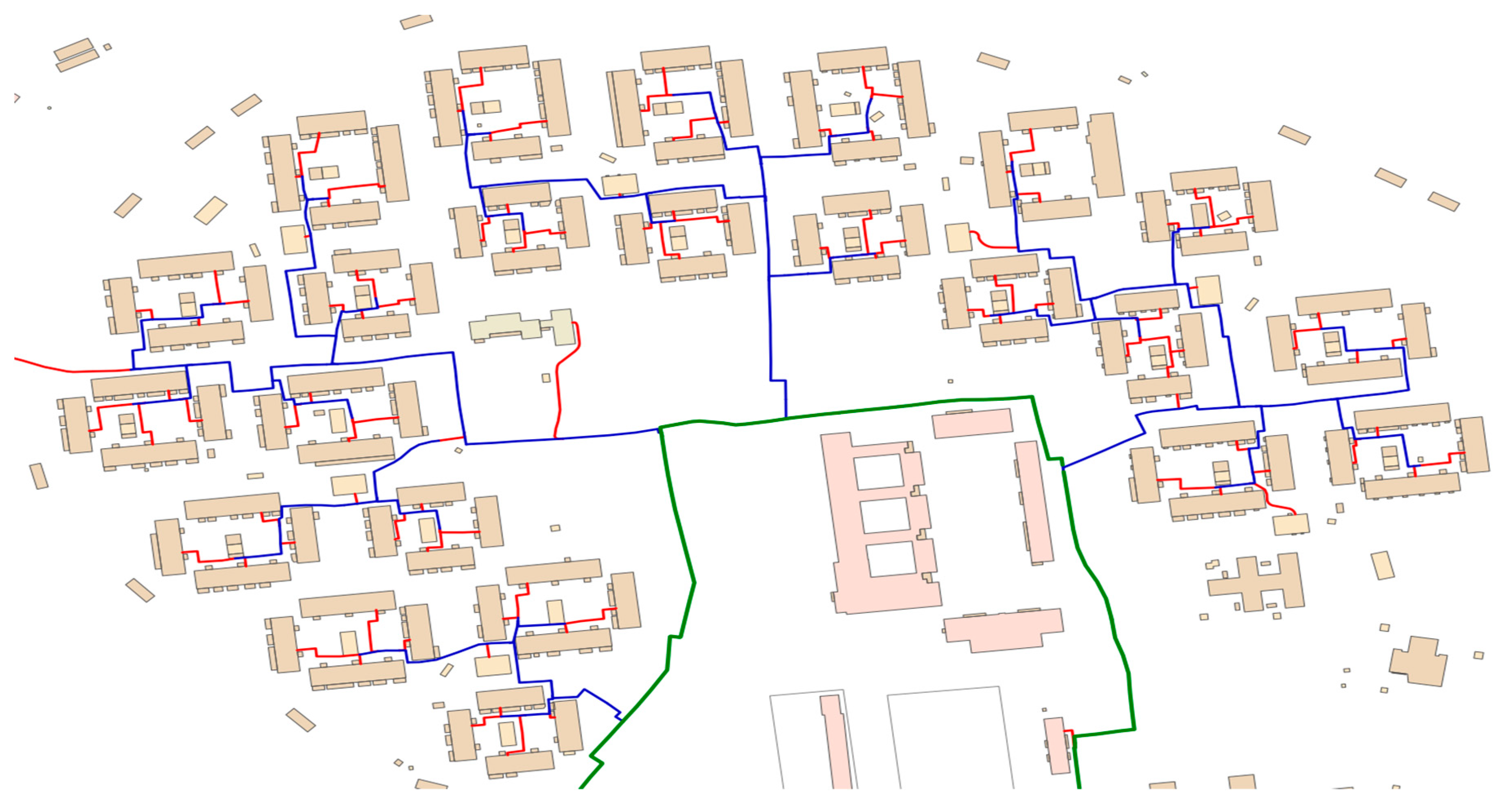
The cost for the distribution network is limited to the service pipe and first order distribution pipes in the neighborhood of the building. Transmission pipes are excluded. The lengths of the service and distribution pipes are based on a typical existing multi-family housing area in Falun, Sweden. Figure 3 shows the distribution network in the district. The average service pipe length is 19 m, and the average distribution length from the service pipe connection to the transmission pipe connection is 280 m for each building. Of these 280 m, 50 m are assumed to have the dimension to cover four buildings, 115 m are assumed to have the dimension to cover 12 buildings, and 115 m are assumed to have the dimension to cover 24 buildings. The average cost for the pipes per building is used in the LCC analysis.
2.3.2. District Heating Production
The DH base load is assumed to be covered using combined heat and power (CHP). The dimension of the CHP plant is based on the daily average peak demand. Two scenarios are considered: One where CHP should cover 40% of the daily average peak demand, and one where it should cover 70%. The daily average peak demand is assumed to be covered by a heat only boiler (HOB). An illustrative picture of these different scenarios is shown in Figure 4. Two different fuels are assumed for the CHP, biomass and municipal waste. These are calculated in different scenarios. In all scenarios, the fuel for the HOB is assumed to be biomass. The biomass fuel cost is based on figures from the Swedish Energy Agency [3], where the CHP fuel is assumed to be a mix of wood chips and forest residue, and the HOB fuel is assumed to be pellets. The cost for the municipal waste is based on figures from a report by the Swedish Energy Research Centre [25].
The average capital cost for the CHP per installed capacity is based upon costs for a 20–80 MW feed plant for the biomass scenario, and a 35–80 MW feed plant for the municipal waste scenario. It is assumed that the CHP plant produces at its maximum all the time. The HOB is dimensioned to cover the additional demand in order to cover the peak demand. The capital costs, O&M costs and the technical parameters, such as lifetime and power-to-heat ratios, are based on Swedish and Danish figures [25,26]. The electricity production in the CHP is credited by the corresponding cost for the electricity production described in Section 2.3.4.
2.3.3. Electricity Distribution
The electricity distribution losses are based on the average for developed countries [24]. With a high share of distributed intermittent production such as wind power, additional investments are needed in the distribution system according to [27]. The investments needed are, for example, a reinforcement of the distribution grid, increased possibilities for demand response flexibility and energy storage. The future electricity production scenarios in [27] are similar to the electricity production scenarios in this article: A high share of wind power with either hydropower or gas turbines as backup power. The average additional cost in the distribution system per installed wind power capacity in [27] is added to the electricity distribution costs in this article.
2.3.4. Electricity Production
The electricity production scenarios are based on two scenarios presented in a report showing possible ways for a 100% renewable Swedish system [27]. The electricity production units consist of wind power and two different kinds of backup power, hydropower and gas turbines, which are considered in different scenarios. The wind power is dimensioned to cover the annual energy demand. The annual electricity production per installed power, together with expected lifetime is based on Danish experience [26]. An average wind power profile for the years 2013–2016 in Sweden, using statistics from the Swedish transmission system operator [28], is compared to the demand profile in order to determine the backup power demand.
In the case of crediting the electricity production from the CHP, the wind power profile is compared to the electricity production profile from the CHP in order to determine the backup power demand. The wind power profile is, in each case, scaled to cover the annual demand and production, respectively.
The capital cost and O&M cost for the wind power is taken from a report by the International Renewable Energy Agency [29]. Corresponding costs for gas turbines as backup power, as well as its technical lifetime and efficiency, are based on average costs for turbines with a capacity of 5–40 MW [25,26]. Bio oil is assumed to be the fuel for the gas turbines, with costs from the Swedish Energy Agency [30]. Hydropower as backup power does not assume completely new hydropower plants. Instead, a capacity increase in existing plants is assumed. The North European Power Perspective has shown that there is a big potential to upgrade the capacity in Swedish hydropower plants [31]. O&M costs and capital costs for the capacity increase, assuming the average costs for turbines of between 10–225 MW, uses figures taken from Krönert et al. [32].
3. Results
The resulting annual energy and peak demand for the building simulation is seen in Table 2. The electricity demand, annual and peak, is increased for all energy renovation measures compared to the reference building. At the same time, the DH demand is decreased, leading to a decreased total annual demand of bought energy.
The total LCC for building renovation measures compared to the reference building for each energy system scenario is shown in Figure 5. None of the renovation measures result in a lower LCC than the reference building for any energy system scenario. The highest increase in LCC is for the four energy system scenarios with gas turbines as backup power. Amongst those scenarios, the scenarios with a higher share of CHP have a higher cost, where biomass as fuel in the CHP results in the highest increase in the LCC.
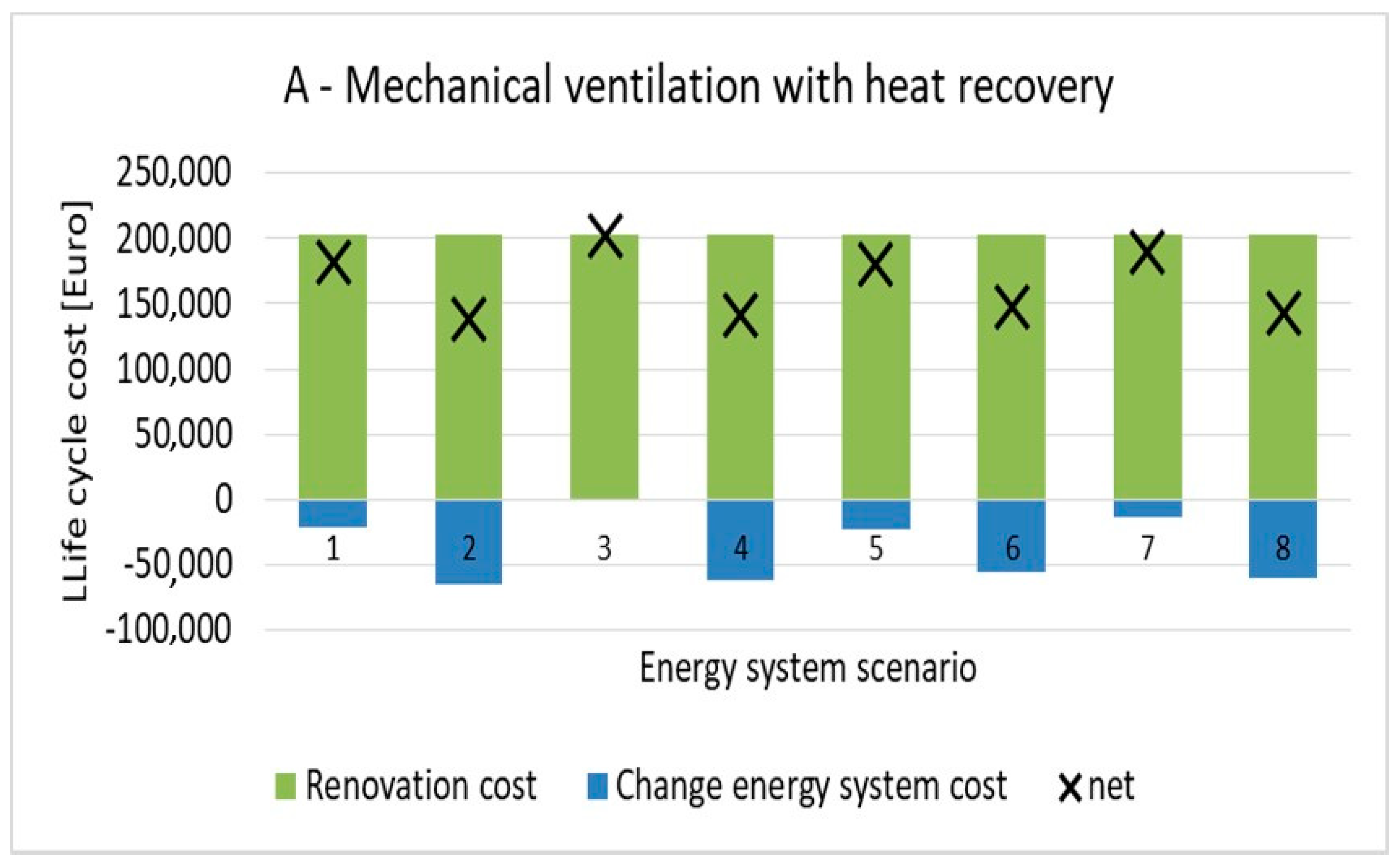
The LCC change in absolute values for each renovation measure, compared to the reference case, is seen in Figure 6, Figure 7 and Figure 8. The LCC change is divided into renovation cost and changes in the energy system cost, for each energy system scenario. Building renovation measure A, mechanical ventilation with heat recovery together with DH, is the only measure which results in a lower energy system cost than the reference case with only DH. The building renovation cost is however high enough to give a net increase in the total LCC. The renovation costs for measures B and C are considerably lower than the cost for system A. However, due to the increased energy system costs for most energy system scenarios, the total LCC is still higher than for the reference building. The energy system cost is only decreased for two energy system scenarios for renovation measure B (scenario 2 and 6), and in one energy system scenario (scenario 2) for renovation measure C.
4. Discussion
The installation of HPs and MVHR are considered economically beneficial from a house owner’s perspective [9,10]. From a wider energy system perspective the situation may look totally different. In this study, the LCC for all three energy renovation measures with either MVHR, or EAHP together with DH, are higher than the LCC for the reference building with DH as the only heat supply. The energy renovation measures decrease the total final energy demand of the building. However, this is at the expense of an increased electricity demand. Electricity is an energy carrier with a higher quality, i.e., higher exergy, than DH, and is often more expensive to produce. Since electricity is a totally different energy carrier than DH, it is also important to separate these in complementary environmental analyses in order to choose both what is the best option from an environmental point of view, and from an economic point of view.
The electricity production in the scenarios is according to possible future scenarios, with wind power dimensioned to cover the annual demand. Due to the intermittent nature of wind power, backup power is needed in order to cover any power demands. Two different kinds of backup power are analyzed, hydropower and gas turbines. Using gas turbines as backup power results in a higher LCC for the renovations measures compared to hydropower as backup power. The cost for the hydropower is, however, calculated as an additional cost for increasing the power capacity of current hydropower stations, for which there is a potential in Sweden according to [31]. Where there is no existing hydropower, the costs need to be changed to the cost for newly built hydropower stations.
A high share of CHP in the DH production is also more favorable economically for DH. CHP plants are more expensive to build than HOBs. The electricity produced in the CHP plant is however credited by the value of the corresponding electricity production from the respective scenario. A high cost for the corresponding electricity production then makes a high share of CHP more economical than a low share.
Biomass-based CHP has a higher LCC for the renovation measures compared to municipal waste-based CHP. Biomass-based CHP has a higher electricity to heat ratio, and the difference compared to municipal waste-based CHP is therefore increased for the scenarios with a high share of CHP and gas turbines as backup power.
For all renovation measures, the renovation has a higher LCC than the reference building. In the case with the MVHR, system A, there is an LCC saving on the energy system side. However, the saving is not higher than the renovation cost, leading to an increased total LCC compared to the reference building. For renovation measures with an EAHP, systems B and C, there is not even a LCC saving on the energy system side when implementing these measures. The reason is as explained above, that the cost for electricity is higher than the cost for DH based on CHP. The MVHR also increased the electricity demand, but the decreased DH demand per increased electricity demand is higher compared to the EAHP systems. Looking at the annual demands, 4–4.5 kWh of DH is saved for each kWh of increased electricity demand in the EAHP systems. System A with MVHR saves around 9 kWh of DH for each kWh of increased electricity demand.
Buildings such as the studied reference case are often in need of more or less extensive renovation, due to age and wear. Renovation of the building envelope (walls, roof and windows) can be combined with measures to improve the indoor climate and the thermal comfort and reduce the heating demand and operating costs, as shown in many previous studies [9,33,34,35,36]. However, it has been argued that for buildings with DH, it is better to focus on reducing the electricity demand than the heating demand, since many DH systems are based on CHP, and the market for heat is more constrained than the market for electricity [37,38,39]. In a wider system perspective, this means that reducing the electricity production from CHP plants would increase the electricity production from other, possibly fossil, energy sources.
All of the studied energy system scenarios are future scenarios. The building renovation measures are however measures that are carried out today throughout Sweden. This is because it is easier to fulfill current building regulation requirements with HPs or combinations of HPs and DH than with DH alone. From a building perspective, these measures are also often economically profitable, based on the energy cost in the current energy system. The current energy system is, however, not 100% renewable. If the energy system should change in order to become 100% renewable, the prices for the property owners would change as well, which is shown in this study. None of the renovation measures have a lower LCC than the reference building with DH, even if they, from a building perspective in the current energy system, can be economically profitable. In a system where the investments have a long technical lifetime and payback time, such as the DH distribution network, there must be a longer time perspective when calculating the economical profitability.
5. Conclusions
The outcome of life cycle calculations of building renovation measures may differ depending on the energy system boundaries considered. In this study, rather than calculating only from a building perspective, a wider perspective regarding the energy system is taken into account, with the system boundary extended to include the complete energy system, as different future scenarios. The life cycle costs for three different energy renovation measures, including HPs and MVHR, have been calculated for a multi-family building and compared to a building with DH alone. All three renovation measures reduce the total energy demand, but at the expense of an increased electricity demand.
Based on the assumptions made for the future energy scenarios, the life cycle cost for renovation measures that increase the electricity demand is higher compared to the reference building, even though the total energy demand is decreased. This shows the importance of including the whole energy system in the calculations, and taking possible future scenarios into consideration.
Author Contributions
Conceptualization, M.S.G. and E.D.; methodology, M.S.G. and M.G.; software, M.S.G. and M.G.; validation, M.S.G. and M.G.; formal analysis, M.S.G.; investigation, M.S.G.; writing—original draft preparation, M.S.G.; writing—review and editing, M.S.G., M.G., E.D. and J.A.M.; visualization, M.S.G.; supervision, E.D. and J.A.M.; project administration, M.SG.
Funding
The work has been carried out under the auspices of the industrial post-graduate school Reesbe, which is financed by the Knowledge Foundation (KK-stiftelsen) and Falu Energi & Vatten AB.
Conflicts of Interest
The authors declare no conflict of interest.
Appendix A

Table A1.
Parameters used for the renovation measure calculations.
| Parameter | Unit | Value | Reference |
|---|---|---|---|
| Exhaust ventilation | |||
| Investment cost * | EUR | 24 000 | [40,41] |
| O&M cost | EUR/y | 240 | * |
| Lifetime | Year | 15 | |
| MVHR system | |||
| Investment cost ** | EUR | 180 000 | [40,41] |
| O&M cost | EUR/y | 1 800 | * |
| Lifetime | Year | 15 | |
| EAHP | |||
| Investment cost ** | EUR | 15 600 | *** |
| O&M cost | EUR/y | 156 | * |
| Lifetime | Year | 20 | |
| EAHP pipes, valves and controller | |||
| Investment cost ** | EUR | 5 400 | *** |
| O&M cost | EUR/y | 54 | * |
| Lifetime | Year | 30 | |
| DHW tank | |||
| Investment cost ** | EUR | 5 500 | [42] |
| O&M cost | EUR/y | 55 | * |
| Lifetime | Year | 20 |
* Operation and Maintenance (O&M) costs are assumed to be 1% of the investment cost; ** Investment costs include costs for installation, based on hourly labor costs [22]; *** Erik Olsson, Thermia, personal contact, 15 May 2015.
Table A2.
Input parameters used for the energy system model.
| Parameter | Unit | Value | Reference |
|---|---|---|---|
| DH distribution | |||
| Cost distribution pipe 100–250 kW | EUR/m | 370 | [24] |
| Cost distribution pipe 250 kW–1 MW | EUR/m | 460 | [24] |
| Cost distribution pipe 1–5 MW | EUR/m | 640 | [24] |
| Cost distribution pipe 5–25 MW | EUR/m | 1 185 | [24] |
| Cost service pipe 50–100 kW | EUR/m | 379 | [24] |
| Cost service pipe >100 kW | EUR/m | 413 | [24] |
| Substation cost <1 MW | EUR/kW | 265 | [24] |
| Lifetime | Year | 40 | [24] |
| O&M cost | EUR/kWh | 0.0015 | [24] |
| Biomass CHP | |||
| Alpha-value | Electricity/heat | 0.35 | [25,26] |
| Specific investment cost | EUR/kWel,net | 5 400 | [25,26] |
| Lifetime | Year | 27.5 | [25,26] |
| O&M fixed | EUR/kWel,net | 189.5 | [25,26] |
| O&M variable | EUR/kWhel,net | 0.0061 | [25,26] |
| Fuel cost | EUR/kWh | 0.016 | [3] |
| Municipal waste CHP | |||
| Alpha-value | Electricity/heat | 0.255 | [25,26] |
| Specific investment cost | EUR/kWel,net | 10 000 | [25,26] |
| Lifetime | Year | 27.5 | [25,26] |
| O&M fixed | EUR/kWel,net | 365.65 | [25,26] |
| O&M variable | EUR/kWhel,net | 0.02535 | [25,26] |
| Fuel cost | EUR/kWh | −0.0125 | [25] |
| Biomass HOB | |||
| Specific investment cost | EUR/kW | 735 | [25,26] |
| Lifetime | Year | 27.5 | [26] |
| O&M fixed | EUR/kW | 22.75 | [25,26] |
| O&M variable | EUR/kWh | 0.0007 | [25,26] |
| Fuel cost | EUR/kWh | 0.025 | [3] |
| Wind power | |||
| Annual electricity production per installed power | kWh/kW | 2 850 | [26] |
| Specific investment cost | EUR/kW | 1 260 | [29] |
| O&M fixed | EUR/kW | 50 | [29] |
| O&M variable | EUR/kWh | 0.026 | [29] |
| Lifetime | Year | 27 | [43] |
| Backup power gas | |||
| Investment cost | EUR/kW | 650 | [25,26] |
| Lifetime | Year | 25 | [25,26] |
| O&M fixed | EUR/kW | 19.5 | [26] |
| O&M variable | EUR/kWh | 0.006 | [26] |
| Fuel cost | EUR/kWh | 0.06 | [30] |
| Efficiency | % | 35 | [25,26] |
| Backup power hydro | |||
| Investment cost | EUR/kW | 265 | [32] |
| Lifetime | Year | 50 | [32] |
| O&M total | EUR/kWh | 0.02 | [32] |
References
- The European Commission. Directive 2010/31/EU on the Energy Performance of Buildings. 2010, pp. 1–35. Available online: https://eur-lex.europa.eu/legal-content/EN/TXT/?uri=CELEX%3A32010L0031 (accessed on 16 July 2019).
- Boverket. wedish Building Code. BFS 2011:6. 2018. Available online: https://www.boverket.se/sv/lag--ratt/forfattningssamling/gallande/bbr---bfs-20116/ (accessed on 16 July 2019).
- Swedish Energy Agency. Energy in Sweden Facts and Figures 2018. 2018. Available online: http://www.energimyndigheten.se/en/facts-and-figures/publications/ (accessed on 16 July 2019).
- Gustafsson, M.; Thygesen, R.; Karlsson, B.; Ödlund, L. Rev-changes in primary energy use and CO2 emissions—An impact assessment for a building with focus on the swedish proposal for nearly zero energy buildings. Energies 2017, 10, 978. [Google Scholar] [CrossRef]
- Gustafsson, M.; Rönnelid, M.; Trygg, L.; Karlsson, B. CO2 emission evaluation of energy conserving measures in buildings connected to a district heating system—Case study of a multi-dwelling building in Sweden. Energy 2016, 111, 341–350. [Google Scholar] [CrossRef]
- Lidberg, T.; Gustafsson, M.; Myhren, J.A.; Olofsson, T.; Ödlund, L. Environmental impact of energy refurbishment of buildings within different district heating systems. Appl. Energy 2018, 227, 231–238. [Google Scholar] [CrossRef]
- Ramírez-Villegas, R.; Eriksson, O.; Olofsson, T. Life Cycle Assessment of Building Renovation Measures—Trade-off between Building Materials and Energy. Energies 2019, 12, 344. [Google Scholar] [CrossRef]
- Le Truong, N.; Gustavsson, L. Costs and primary energy use of heating new residential areas with district heat or electric heat pumps. Energy Procedia 2019, 158, 2031–2038. [Google Scholar] [CrossRef]
- Gustafsson, M.; Swing Gustafsson, M.; Myhren, J.A.; Bales, C.; Holmberg, S. Techno-economic analysis of energy renovation measures for a district heated multi-family house. Appl. Energy 2016, 177, 108–116. [Google Scholar] [CrossRef] [Green Version]
- Paiho, S.; Pulakka, S.; Knuuti, A. Life-cycle cost analyses of heat pump concepts for Finnish new nearly zero energy residential buildings. Energy Build. 2017, 150, 396–402. [Google Scholar] [CrossRef]
- Statistics Sweden Number of Dwellings by Region, Type of Building and Period of Construction. Available online: https://www.scb.se/en/finding-statistics/statistics-by-subject-area/housing-construction-and-building/housing-construction-and-conversion/dwelling-stock/ (accessed on 2 July 2019).
- Hall, T.; Vidén, S. The Million Homes Programme: A review of the great Swedish planning project. Plan. Perspect. 2005, 20, 301–328. [Google Scholar] [CrossRef]
- ISO. ISO 15686-5:2017—Buildings and Constructed Assets—Service Life Planning—Part 5: Life Cycle Costing; ISO: Geneva, Switzerland, 2017. [Google Scholar]
- CEN. EN 15459-1:2017—Energy Performance of Buildings—Economic Evaluation Procedure for Energy Systems in Buildings—Part 1: Calculation Procedures, Module M1-14; European Committee for Standardization: Brussels, Belgium, 2017. [Google Scholar]
- Lund, R.; Ilic, D.D.; Trygg, L. Socioeconomic potential for introducing large-scale heat pumps in district heating in Denmark. J. Clean. Prod. 2016, 139, 219–229. [Google Scholar] [CrossRef] [Green Version]
- Lund, R.; Skaarup Östergaard, D.; Yang, X.; Vad Mathiesen, B. Comparison of Low-Temperature District Heating Concepts in a Long-Term Energy System Perspective. Int. J. Sustain. Energy Plan. Manag. 2017, 12, 5–18. [Google Scholar]
- Swing Gustafsson, M.; Gustafsson, M.; Myhren, J.A.; Dotzauer, E. Primary energy use in buildings in a Swedish perspective. Energy Build. 2016, 130, 202–209. [Google Scholar] [CrossRef]
- Andreasson, M.; Borgström, M.; Werner, S. Värmeanvändning i Flerbostadshus Och Lokaler 2009:4; Svensk Fjärrvärme: Stockholm, Sweden, 2009. [Google Scholar]
- Thermia Thermia Mega XL (in Swedish). Available online: http://www.thermia.se/produkter/thermia-mega.asp (accessed on 9 February 2015).
- Klein, S.; Beckman, A.; Mitchell, W.; Duffie, A. TRNSYS 17—A TRansient SYstems Simulation Program; Solar Energy Laboratory: Zoetermeer, The Netherlands; University of Wisconsin: Madison, WI, USA, 2011. [Google Scholar]
- Meteonorm. Global Meteorological Database for Engineers, Planners and Education. Available online: http://meteonorm.com/ (accessed on 15 October 2015).
- Eurostat. Labour costs annual data—NACE Rev.2. European Commission, 2018. Available online: https://ec.europa.eu/eurostat/web/products-datasets/-/tps00173 (accessed on 16 July 2019).
- Swing Gustafsson, M.; Myhren, J.A.; Dotzauer, E. Life cycle cost of heat supply to areas with detached houses—A comparison of district heating and heat pumps from an energy system perspective. Energies 2018, 11, 3266. [Google Scholar] [CrossRef]
- Danish Energy Agency; Energinet. Technology Data for Energy Transport. 2017. Available online: https://ens.dk/en/our-services/projections-and-models/technology-data/technology-data-energy-transport (accessed on 16 July 2019).
- Nohlgren, I.; Herstad Svard, S.; Jansson, M.; Rodin, J. Electricity from New and Future Plants Elforsk Rapport 14:45; Elforsk: Stockholm, Sweden, 2014. [Google Scholar]
- Danish Energy Agency; Energinet. Technology Data for Energy Plants for Electricity and District Heating Generation. 2018. Available online: https://ens.dk/en/our-services/projections-and-models/technology-data/technology-data-generation-electricity-and (accessed on 16 July 2019).
- Krönert, F.; Bruce, J.; Jakobsson, T.; Badano, A.; Helbrink, J. 100% Förnybart—En Rapport till Skellefteå Kraft (100% Renewable, in Swedish). 2017. Available online: https://www.skekraft.se/wp-content/uploads/2017/06/100_procent_fornybart_2040.pdf (accessed on 16 July 2019).
- Svenska Kraftnät Electricity Market—Statistics. Available online: https://www.svk.se/aktorsportalen/elmarknad/statistik/ (accessed on 13 September 2018).
- International Renewable Energy Agency. Renewable Power Generation Costs in 2017; IRENA: Abu Dhabi, UAE, 2018. [Google Scholar]
- Swedish Energy Agency. Övervakningsrapport Avseende Skattebefrielse för Vissa Biobränslen vid Användning som Bränsle för Uppvärmning år 2016. 2017. (In Swedish). Available online: http://epi6.energimyndigheten.se/PageFiles/54547/%C3%96vervakningsrapport%20avseende%20skattebefrielse%20f%C3%B6r%20flytande%20biodrivmedel%202016%202016-12009.pdf (accessed on 16 July 2019).
- North European Power Perspective, N. Stor Potential för Effekthöjning i Svensk Vattenkraft (in Swedish, “Great Potential for Power Increase in Swedish Hydropower”). Available online: http://nepp.se/pdf/Stor_potential_effekthojning.pdf (accessed on 21 March 2019).
- Krönert, F.; Helbrink, J.; Marklund, J.; Edfeldt, E.; Walsh, R.; Bitar, F.; Holtz, C.; Bruce, J. Ekonomiska Förutsättningar för Skilda Kraftslag (in Swedish, “Economic Conditions for Different Power Sources”); Sweco Energuide AB: Stockholm, Sweden, 2016. [Google Scholar]
- Dodoo, A.; Gustavsson, L.; Tettey, U.Y.A. Final energy savings and cost-effectiveness of deep energy renovation of a multi-storey residential building. Energy 2017, 135, 563–576. [Google Scholar] [CrossRef]
- Fotopoulou, A.; Semprini, G.; Cattani, E.; Schihin, Y.; Weyer, J.; Gulli, R.; Ferrante, A. Deep renovation in existing residential buildings through façade additions: A case study in a typical residential building of the 70s. Energy Build. 2018, 166, 258–270. [Google Scholar] [CrossRef]
- Thomsen, K.E.; Rose, J.; Mørck, O.; Jensen, S.Ø.; Østergaard, I.; Knudsen, H.N.; Bergsøe, N.C. Energy consumption and indoor climate in a residential building before and after comprehensive energy retrofitting. Energy Build. 2016, 123, 8–16. [Google Scholar] [CrossRef]
- Földváry, V.; Bukovianska, H.P.; Petráš, D. Analysis of Energy Performance and Indoor Climate Conditions of the Slovak Housing Stock before and after Its Renovation. Energy Procedia 2015, 78, 2184–2189. [Google Scholar] [CrossRef]
- Difs, K.; Bennstam, M.; Trygg, L.; Nordenstam, L. Energy conservation measures in buildings heated by district heating—A local energy system perspective. Energy 2010, 35, 3194–3203. [Google Scholar] [CrossRef]
- Åberg, M.; Henning, D. Optimisation of a Swedish district heating system with reduced heat demand due to energy efficiency measures in residential buildings. Energy Policy 2011, 39, 7839–7852. [Google Scholar] [CrossRef]
- Lundström, L.; Wallin, F. Heat demand profiles of energy conservation measures in buildings and their impact on a district heating system. Appl. Energy 2016, 161, 290–299. [Google Scholar] [CrossRef] [Green Version]
- Ruud, S. Economic Heating Systems for Low Energy Buildings—Calculation, Comparison and Evaluation of Different System Solutions; Contract No.: SP Report 2010:43; SP Technical Research Institute of Sweden: Boras, Sweden, 2010. [Google Scholar]
- Wahlström, Å. Teknikupphandling av Värmeåtervinning i Befintliga Flerbostadshus—Utvärdering; BeBo: Stockholm, Sweden, 2014. [Google Scholar]
- NIBE DHW Preparation Tank. Available online: http://www.nibe.se/Produkter/Ackumulatortankar/Produktsortiment/AKIL/ (accessed on 2 March 2015).
- Danish Energy Agency; Energinet. Technology Data for Individual Heating Installations. 2018. Available online: https://ens.dk/en/our-services/projections-and-models/technology-data/technology-data-individual-heating-plants (accessed on 16 July 2019).
Figure 1.
Flowchart describing the methodology.

Figure 2.
The eight different energy system scenarios regarding electricity and district heating production. In all of these, wind power is dimensioned to cover the annual electricity demand, and biomass-based heat only boilers (HOB) are assumed to cover the district heating peaks.
Figure 2.
The eight different energy system scenarios regarding electricity and district heating production. In all of these, wind power is dimensioned to cover the annual electricity demand, and biomass-based heat only boilers (HOB) are assumed to cover the district heating peaks.

Figure 3.
The distribution network. Red—service pipes, blue—distribution pipes, green—transmission pipes.
Figure 3.
The distribution network. Red—service pipes, blue—distribution pipes, green—transmission pipes.

Figure 4.
Heat load diagrams (where the hourly load over the period of one year is shown with the greatest load to the left and the smallest one to the right, for each scenario) of two different dimensions of combined heat and power (CHP). The scenarios corresponding to the respective CHP dimension are in brackets.

Figure 5.
The life cycle cost (LCC) for the energy renovation measures A—mechanical ventilation with heat recovery, B—exhaust air heat pump for heating and C—exhaust air heat pump for heating and domestic hot water in relation to the reference building, for eight different energy system scenarios. Blue color—biomass based district heating, green color—municipal waste based district heating, square—low share of combined heat and power, circle—high share of combined heat and power, filled—hydropower as electrical backup power, not filled—gas turbines as electrical backup power.

Figure 6.
Life cycle cost for renovation measure A (mechanical ventilation with heat recovery) compared to the reference case, for all eight energy system scenarios. The bars are divided into building renovation cost and changes in energy system costs, with the net cost for each energy system scenario shown as crosses.

Figure 7.
Life cycle cost for renovation measure B (exhaust air heat pump for heating only) compared to the reference case, for all eight energy system scenarios. The bars are divided into building renovation cost and changes in energy system costs, with the net cost for each energy system scenario shown as crosses.

Figure 8.
Life cycle cost for renovation measure C (exhaust air heat pump for heating and hot water) compared to the reference case, for all eight energy system scenarios. The bars are divided into building renovation cost and changes in energy system costs, with the net cost for each energy system scenario shown as crosses.

Table 1.
The different heating and ventilation included in the energy renovation measures. X denotes the heating and ventilation solutions included in each system (reference, A, B and C).
Table 1.
The different heating and ventilation included in the energy renovation measures. X denotes the heating and ventilation solutions included in each system (reference, A, B and C).
| Heating and Ventilation System | Ref. | A | B | C |
|---|---|---|---|---|
| Mechanical ventilation | X | X | X | X |
| Mechanical ventilation with heat recovery | X | |||
| Exhaust air heat pump used for heating | X | X | ||
| Exhaust air heat pump used for domestic hot water | X | |||
| District heating | X | X | X | X |
Table 2.
The annual and peak energy demand for the reference building and the three energy renovation measures: A—Mechanical ventilation with heat recovery, B—Exhaust air heat pump for heating and C—Exhaust air heat pump for heating and domestic hot water in relation to the reference building.
Table 2.
The annual and peak energy demand for the reference building and the three energy renovation measures: A—Mechanical ventilation with heat recovery, B—Exhaust air heat pump for heating and C—Exhaust air heat pump for heating and domestic hot water in relation to the reference building.
| Heating System | Ref. | A | B | C |
|---|---|---|---|---|
| District heating | ||||
| Annual demand [MWh] | 655 | 515 | 480 | 451 |
| Daily average peak demand [kW] | 215 | 169 | 173 | 173 |
| Electricity | ||||
| Annual demand [MWh] | 21 | 36 | 63 | 67 |
| Hourly average peak demand [kW] | 4 | 6 | 18 | 18 |
| Total annual demand [MWh] | 676 | 551 | 543 | 518 |
© 2019 by the authors. Licensee MDPI, Basel, Switzerland. This article is an open access article distributed under the terms and conditions of the Creative Commons Attribution (CC BY) license (http://creativecommons.org/licenses/by/4.0/).
Share and Cite
MDPI and ACS Style
Gustafsson, M.S.; Myhren, J.A.; Dotzauer, E.; Gustafsson, M. Life Cycle Cost of Building Energy Renovation Measures, Considering Future Energy Production Scenarios. Energies 2019, 12, 2719. https://doi.org/10.3390/en12142719
AMA Style
Gustafsson MS, Myhren JA, Dotzauer E, Gustafsson M. Life Cycle Cost of Building Energy Renovation Measures, Considering Future Energy Production Scenarios. Energies. 2019; 12(14):2719. https://doi.org/10.3390/en12142719
Chicago/Turabian StyleGustafsson, Moa Swing, Jonn Are Myhren, Erik Dotzauer, and Marcus Gustafsson. 2019. "Life Cycle Cost of Building Energy Renovation Measures, Considering Future Energy Production Scenarios" Energies 12, no. 14: 2719. https://doi.org/10.3390/en12142719
Note that from the first issue of 2016, this journal uses article numbers instead of page numbers. See further details here.