Wind Farm Modeling with Interpretable Physics-Informed Machine Learning


1
Department of Mechanical Engineering, Stanford University, Stanford, CA 94305, USA
2
Department of Civil and Environmental Engineering, Stanford University, Stanford, CA 94305, USA
*
Author to whom correspondence should be addressed.
Energies 2019, 12(14), 2716; https://doi.org/10.3390/en12142716
Submission received: 29 May 2019
/
Revised: 8 July 2019
/
Accepted: 10 July 2019
/
Published: 16 July 2019
(This article belongs to the Special Issue State of the Art of Wind Farm Optimization)
Abstract
:Turbulent wakes trailing utility-scale wind turbines reduce the power production and efficiency of downstream turbines. Thorough understanding and modeling of these wakes is required to optimally design wind farms as well as control and predict their power production. While low-order, physics-based wake models are useful for qualitative physical understanding, they generally are unable to accurately predict the power production of utility-scale wind farms due to a large number of simplifying assumptions and neglected physics. In this study, we propose a suite of physics-informed statistical models to accurately predict the power production of arbitrary wind farm layouts. These models are trained and tested using five years of historical one-minute averaged operational data from the Summerview wind farm in Alberta, Canada. The trained models reduce the prediction error compared both to a physics-based wake model and a standard two-layer neural network. The trained parameters of the statistical models are visualized and interpreted in the context of the flow physics of turbulent wind turbine wakes.
1. Introduction
To prevent global averaged temperatures from rising 1.5 °C above pre-industrial levels, renewable energy must increase from to of global energy production from 2018 to 2040 [1]. To meet this goal, wind farms are increasing in size and energy production penetration. With increasing wind turbine and wind farm size, the costs of high voltage transmission lines and land usage increase significantly [2]. As such, wind farms are typically constructed with a streamwise spacing of 6–10 turbine diameters in the prevailing wind direction [3]. With these average distances between turbines, downstream turbines produce significantly less power than freestream turbines as a result of aerodynamic wake effects when wind speeds are below the rated value [4]. Due to the loss in wind farm efficiency as a result of wind turbine wakes, numerous works have attempted to understand the governing physics of this phenomena in an effort to model the power production of wind farms [5]. The complex interactions between wind farms and the atmospheric boundary layer have been well studied, as recently reviewed by Stevens and Meneveau [6].
Physical observations and simulations have led to a number of wind turbine wake models which aim to accurately capture the aerodynamics of a single wind turbine wake. Such wake models show good agreement for single turbines with wind tunnel experiments [7], numerical simulations [8], and field experiments [9]. However, the aerodynamic interactions within wind farm models remain challenging to capture as a result of wake superposition [10], boundary layer interactions [6,11], complex terrain [12], Coriolis forces [13], deep array effects [14,15], and other neglected physics. When wind turbines are tightly spaced in a wind farm, the individual turbine wakes merge into a large wind farm wake [16]. Wind farm wakes may extend over tens of kilometers and have been shown to influence downwind wind farms [17,18,19]. Van der Laan et al. [20] used Reynolds Averaged Navier–Stokes simulations to predict the magnitude of interaction between two wind farms as a result of the merged wind farm wake. While this merging effect can be captured using computationally expensive simulations such as numerical weather prediction or large-eddy simulation, it is challenging to capture with low-order wake models [17]. As a result of these complexities, contemporary studies typically rely on high-fidelity numerical simulations [21]. While physics-based wake models are able capture the qualitative trends of wind farm power production [4,6], quantitative predictions of power production remain inaccurate as a result of wake model simplifications. The complexities of incorporating these phenomena in large wind farm models was recently reviewed by Sanz Rodrigo et al. [22].
Recent developments in neural network based machine learning have led to a significant leap in the ability for statistical approaches to model complex datasets (see, e.g., [23,24]). Deep neural network approaches have provided useful insights when informed by the governing physics of fluid mechanics [25]. However, deep neural networks are challenging to interpret [26], which leads to uncertainty in the ability of the models to generalize across different datasets and difficulty in establishing new physical insights. Recent work [27,28] has shown the ability for statistical models to efficiently maximize wind farm power production in a control oriented approach with a physics-driven wake model. Further, neural networks have been used extensively to improve wind farm power forecasting (see, e.g., [29,30,31]). Due to the known deficiencies of low-order wake models in capturing the complex physics of utility-scale wind farms and given the recent successes of statistical approaches to model wind farm power production, we propose a statistically driven wake model. The statistical model is guided through physical insight to reduce overfitting and aid in robustness.
In Section 2, interpretable physics-informed statistical wake models are proposed as well as a previously developed physics-driven low-order wake model for comparison. The various models are compared in Section 3 in the analysis of a utility-scale wind farm in Alberta, Canada. Physical interpretations of the statistical model are given in Section 4 and conclusions are given in Section 5.
2. Wind Farm Power Models
The development of accurate, computationally efficient power production models is particularly useful in the study of wind farms due to their widespread use in layout optimization [32,33] and active-control [34,35,36,37]. Low-order wind farm models continue to be relevant for engineering applications due to the computational expense of fully-resolved [38] or even large-eddy simulations [39]. While physics-driven wake models are predominantly used in control oriented approaches [40], statistical machine learning models have been utilized for the purpose of power forecasting (see, e.g., [41]). In this section, we review a physics-based model and propose a suite of statistical models for the purpose of control- and design-oriented wake prediction.
2.1. Physics-Based Model
Physics-driven analytic wake models have been extensively applied for the purpose of wind farm power prediction [5]. While such analytic models are lower in reliability than high fidelity simulations, they can accurately capture wind farm power production trends [4]. Low-order models are particularly relevant for the purpose of online control of wind farm power as a function of time for energy grid optimization (see, e.g., [42,43,44]) due to the computational expensive of online large-eddy simulations [45]. The physics-based, low-order model selected here is the Gaussian wake model [7] with the momentum theory prescribed by Prandtl’s lifting line model [8]. The Gaussian wake model is selected due to its success in reproducing the power production for field tests of utility-scale turbines [37] while the lifting line model is chosen since it is suitable for wake steering control optimization [8,44]. The streamwise velocity following a single wind turbine i is modeled as
where D is the turbine diameter, is the proportionality constant of the presumed Gaussian wake, is the normalized diameter of the wake, the streamwise velocity at the most upwind turbine is , x is the streamwise direction, and is the lateral direction in the frame of the upwind turbine. The lateral centroid of the wake is . The streamwise velocity deficit is prescribed by a lifting line model given by [8]:
where with a giving the axial induction factor from actuator disk theory (e.g., [46]).
While low-order models have significantly less computational complexity than turbulence simulations, computational efficiency is still required due to the large parameter space of layout or yaw optimization [47]. The dominant factor in the computational cost of low-order models is the spatial domain discretization, whereby the low-order model is solved at all grid points in a computational domain. As such, Howland et al. [44] developed an analytic power function to predict wind turbine power production for an arbitrary wind farm layout and yaw misalignment without requiring domain discretization. This method is at least two orders of magnitude less computationally complex than previously used low-order models of similar fidelity. Using linear wake superposition, the effective, area-averaged velocity at a turbine j in an arbitrary wind farm can be modeled as
where the downstream turbine lateral center is . The deficit of velocity is computed as the linear superposition of all upstream turbines [48]. The power is then computed as
where is the density of air and is the turbine area. The coefficient of power is a function of the wind speed and is given by .
Due to the inherent nonlinearity of the wind turbine wakes as a function of the wind speed, the analytic model requires model coefficients, which are a function of the wind speed [44]. For lower wind speeds, wind turbines maximize power production and strong wakes are produced (i.e., and the downstream turbine produces significantly less power than the upstream turbine). Above the rated wind speed, power production does not increase above the rated value and turbines will extract a reduced fraction of the incoming wind power [49]. Therefore, above the rated wind speed, weak turbulent wakes are produced (i.e., and the downstream turbine produces similar power to the upstream turbine). Since the model relies on the computation of these physical turbulent wakes, it is not able to sufficiently generalize across the dataset for all wind speeds where the strength of the wakes will vary. As a result, larger modeling errors may persist when the physics-driven wake model is fit for all wind speeds rather than fitting specifically to narrow wind speed bins.
The wake spreading coefficient and the proportionality constant of the Gaussian wake is prescribed for each wind turbine in the wind farm based on historical data. As a result, there are trainable parameters, where is the number of turbines in the wind farm. The parameters are trained using analytic gradients [44] combined with a genetic algorithm summarized in Algorithm 1. The model is calibrated for an arbitrary wind farm separately for each wind direction bin between 0° and 360°. The model must be calibrated separately for each wind direction since the effective layout of the wind farm is a function of the wind direction. While the same wake parameters are used for all wind speeds, the model is run for each temporal instance in the historical data since the physics-based model dynamics are dependent on the inflow wind speed (e.g., ).
The genetic algorithm minimization MinError takes in the historical baseline data P and the initialized wake spreading rate and proportionality constant of the Gaussian wake, and , respectively. The algorithm also requires the coordinates of the wind turbines. The number of parents in the algorithm is N, the number of parents selected for the next generation is k, and and are the standard deviations of the mutation perturbations applied to the children. The Forward algorithm is the lifting line model described by Equations (3) and (4). The Forward algorithm requires the turbine coordinates within the wind farm which are given by X. The error is computed as a mean absolute error (MAE)
where is the absolute value operator and is the average over the turbines in the wind farm. The analytic gradients are computed using the Backward algorithm, which uses a computational graph to compute gradients based on the parametric state of the model (see, e.g., [23] for a review). The parameters are updated using Adam gradient descent [50] using GradientUpdate. Once all parents (N) have been iterated through, the k parents with the lowest error e are selected using Select. The new parents are created using a CrossOver algorithm, which averages two randomly selected parents from the k best performers to create N new parents. Finally, Gaussian noise with zero mean and standard deviations and are added to the new parents in Mutate. Once the MAE () reaches the desired threshold TOL, the algorithm is terminated and the best parameters , are returned. Numerical experiments resulted in the selection of , , , , and . In the present study, the tolerance parameter TOL was not set and all training ran until .
| Algorithm 1 Genetic algorithm gradient descent minimization of mean absolute error of lifting line model. |
| MinError(P,, , X, N, k, , ): |
| while TOL and do |
| for do |
| Forward() |
| MAE(, P) |
| , Backward(, ) |
| GradientUpdate(,) |
| end for |
| , , Select(, , , k) |
| if then |
| end if |
| , CrossOver(, ) |
| , Mutate(, , , , ) |
| end while |
| return, |
2.2. Physics-Informed Statistical Model
In large wind farm configurations that contain significant streamwise spacing, low-order wake models are generally less accurate (see, e.g., [6]). In particular, the wake interaction of far wakes and their inherent merging into a so-called wind farm wake is typically not well captured by the traditional forms of wake superposition [51]; additionally, large-scale atmospheric boundary layer (ABL) structures [52,53], which influence mixing and wake decay, are typically neglected [6]. As a result, in this section, we revisit the predominant cause of the power model breakdown, namely the modeling of streamwise velocity deficit as a function of downstream position.
Following the assumptions of inviscid flow, neglecting Coriolis and stratification effects, linearizing the advection term, and Reynolds-averaging, the momentum equation governing the transport of is
where is the pressure, is the turbine forcing, and is the Reynolds stress tensor [8]. Parameterizing the wake with a spreading coefficient and area averaging results in an ordinary differential equation in x which can be analytically solved to give Equation (2). While the prescription of follows inviscid theory, the solution of Equation (6) requires a significant number of assumptions and parameterizations. Further, upon solution, the velocity deficits within a multi-turbine wind farm must be then superposed in an ad-hoc method, which is not necessarily based on physical laws of conservation [6]. Finally, the functional form of given by Equation (2) is diminished in accuracy in the far wake due to the linearization of the advection term.
As a result, we propose to utilize data-driven machine learning to inform the wind farm power production. We determine which turbines are well-correlated through the minimization of a loss-based objective function. In particular, wind turbine power is modeled as
where is the number of turbines in front of turbine i. In Equation (7), the power prediction for a downstream turbine is a linear regression based on the power generated by upstream turbines. A sketch of the statistical model architecture can be seen in Figure 1. This is similar to the construction of a directed acyclic graph [54] where we construct a connectivity among the turbines within the wind farm. An upstream turbine j is connected to all subsequent downstream turbines i with a corresponding weight value, . This model architecture is similar to multi-dimensional linear ordinary least squares with an objective function of MAE (least absolute deviations) instead of square residual minimization. A unique solution is not guaranteed with least absolute deviations but solutions are typically more robust [55] than least squares (see Appendix A and Appendix B).
However, spatiotemporal wind turbine wake interactions are inherently variable and nonlinear as a function of wind speed [56,57]. The wind turbine thrust coefficient is a function of the wind speed, as shown in Figure 2. At low wind speeds, the coefficient of thrust is high, as shown in Figure 2a, and the wake losses will be large. As the wind speed approaches 15 m/s, where rated power occurs, the sharply decreases and wake losses will be small since wakes will not be driven by the turbine induction. Therefore, the linear fit given by Equation (7) may not capture wake interactions that are a function of the incoming wind speed.
One method to adequately compensate for these nonlinearities would be to generate separate weight values for separate wind speed bins, i.e., weight values for wind speeds of 5–6 m/s, separate values for wind speeds of 14–15 m/s and so on. On the other hand, various turbines within the wind farm may operating at different points on the curve for a fixed time. Another method to introduce such nonlinearities in a strictly data-driven approach is to implement a neural network architecture. The typical nonlinearities implemented in multi-layer neural networks are the sigmoid function and the rectified linear unit (ReLU) [23]. However, mutlilayer neural networks with an arbitrary number of weights are notoriously difficult to interpret [26] and pose a significant disadvantage when compared to the simplicity of Equation (7). Further, larger neural networks are subject to overfitting to the training set and regularization is typically required [23]. In the present case, the wind turbine control systems present a consistent nonlinearity via the dependence of on wind speed, which can be utilized directly in the model. As such, a sigmoid-type activation function was tuned to the curve as a function of the power generation. The resulting sigmoid-type function is
where is for numerical stability. The input P is the power of a turbine given in MW and is therefore bounded by 0 and 1.8 for the 1.8 MW Vestas V80 turbines. The parameters in the sigmoid-type function were tuned heuristically such that approximately followed . The results were not significantly sensitive to the tuning parameters given a function bounded by 0 and 1 and is approximately zero valued at and . The tuned sigmoid-type function compared to the nonlinearity can be seen in Figure 2b. The resulting wind power model is
where k and c are learnable matrices. While the learnable parameters are unbounded and arbitrary valued, a premultiplier of was used to reduce the occurrence of saddle points in the training process. The nonlinearity can also be replaced with a standard sigmoid nonlinearity which is not tuned to . The weight vectors for turbine i are . The parameter is active at lower wind speeds and is active at higher wind speeds. The nonlinear Equation (9) is tested with in Equation (8) and the standard Sigmoid function (). Additionally, these model performances are compared to a standard two-layer neural network [58]
where now the weights matrices (, ) and the biases (, ) are not the same dimensionality. In particular, the weight vectors for turbine i are and . The biases for turbine i are and . Therefore, Equation (10) has learnable parameters for each turbine while Equation (9) has only learnable parameters. A standard neural network nonlinearity such as the sigmoid or ReLU functions is represented by . The present study focused on the ReLU nonlinearity. A premultiplier was not used in the neural network approach since this architecture is less subject to saddle points due to the high dimensional space of the trainable parameters. Deep neural networks were not tested in the present study due to the large number of learnable parameters in these methods, the associated tendency to overfit to the training data, and the challenge of interpretability [26]. The trainable parameters for all statistical methods introduced here and their associated degrees of freedom are summarized in Table 1.
Wake models are typically constructed to accurately represent the streamwise velocity deficit [5,59] based on a known freestream velocity condition. This approach simplifies the modeling endeavor to a characterization of the small deviations from the known freestream velocity rather than a reconstruction of an unknown velocity signal. Such an approach can be seen in Equation (3), where the is known and the model coefficients dictate , the velocity deficit. To reduce the modeling effort required for the statistical model approaches, a data-driven model based on the deficit of power is constructed
where is the power production of the wind turbine operating at . A premultiplier of was selected for the deficit approach to place the summation term in the same order of magnitude as . The statistical deficit model given by Equation (11) is linear. A similar deficit model can be constructed using the coefficient of thrust based nonlinearity used in Equation (9)
With the specified architectures, the weights and biases summarized in Table 1 can be found through analytic gradient descent optimization. The loss function used for optimization was MAE and the weight matrix was optimized using analytical backpropagation with an Adam optimizer [50] with the standard values of the learning rate , , and . Numerical algorithms were implemented in the machine learning package PyTorch [60] in Python.
2.3. Physics-Informed Initialization
The initialization of weights and biases in neural networks is one of the foremost challenges in the complexity of the models [61]. Poor initialization leads to slow or stalled training and insufficient model performance [50]. The problem is particularly paramount due to the non-convexity of the optimization problem which subjects it to local minima (saddles in high dimensions). While deep networks are, in general, not sensitive to local minima [23], this is not the case in small or shallow networks (e.g., two-layer neural networks). In machine learning problems with physical applications, we can select an initialization which is based on the physical understanding of the problem. Such a selection is similar to the choice of a prior statistical distribution in Bayesian networks [54].
Wakes of objects in turbulent flows exhibit a Gaussian shape in the transverse direction in the far field [6]. Wind turbines in the turbulent ABL have also been shown to exhibit a Gaussian velocity deficit profile in the transverse direction [62]. As a result, single wind turbine wakes are often modeled as a velocity deficit spread along a Gaussian kernel [7]. While the Gaussian wake profile becomes less clear when wakes merge and are superposed within a wind farm [13], it remains a helpful starting point for modeling [63]. Further, as a result of conservation of mass, the wake will expand downstream of the turbine. While the expansion of the wake diameter is still an open question and likely depends on the magnitude of atmospheric turbulence [64] and the type of stratification [6,44], it will likely serve as a useful initial condition for the statistical models.
Following the hypothesis that wakes are Gaussian, the weight value connecting two turbines was initialized as
Incorporating the wake spreading rate in the weight initialization did not significantly influence the results.
2.4. Statistical Model Development Set Protocol
Statistical model parameters were calibrated using a training set and tested for generalization using the development set. With very large datasets, it is common to leave less than of the examples for validation (see, e.g., [65]). The present dataset was split into training, development, and testing sets as per the typical convention of statistical modeling approaches. The dataset was split such that approximately one third of the data points are within each of the training, development, and testing sets. The training, development, and testing sets were split such that they do not share data samples from the same day. This reduces the ability for the model to successfully overfit to specific features given limited data samples [24]. Since the statistical models are unbounded and unconstrained by physics, they can generally reproduce the training dataset arbitrarily well if sufficiently flexible. The development set was used to evaluate the statistical models during training but was not used for the calculation of gradients during the training process. The testing set was not tested until the final model was selected to reduce training bias. While no explicit regularization was incorporated into any of the statistical learning frameworks, early stopping was used where the trained set of parameters with the lowest development set error was selected rather than the set of parameters with the lowest training error.
The statistical models rely on power production information for all upstream turbines to make a prediction of the power production of a downstream turbine. After training, the physics-based model only requires the wind speed () incident on the turbine furthest upstream to make power predictions for all turbines within the wind farm. A standard development set protocol was established for the statistical models to ensure a valid comparison between the physics-based and data-driven approaches. For the development set testing with the statistical models, only the power production data of the most upstream turbine were given to the model. The power production predictions were then used for successive predictions as the model propagates downwind for all turbines.
The models were trained on all wind speeds but the training and development errors are shown for below selected wind speed ranges. Wind speeds above the rated wind speed of 15 m/s were not included because these training examples artificially reduce the MAE for all architectures. This artificial reduction occurs because, above the rated wind speed, nearly all turbines within the wind farm are producing rated power and there are not significant wake losses.
For the physics-based lifting line model, the parameters which give the best performance on the training set were utilized for the model comparisons. For the statistical models, while the parameters were learned from the training dataset, the parameters with the best performance on the development set were taken as the standard machine learning protocol [23].
3. Model Evaluation on Utility-Scale Wind Farm
To validate the potential of the physics-informed statistical methods to model wind farm power production, the aforementioned suite of physics-driven and statistical models were tested using supervisory control and data acquisition (SCADA) data. The operational wind farm data are described in Section 3.1 and the models are compared in Section 3.2.
3.1. Utility-Scale Wind Farm
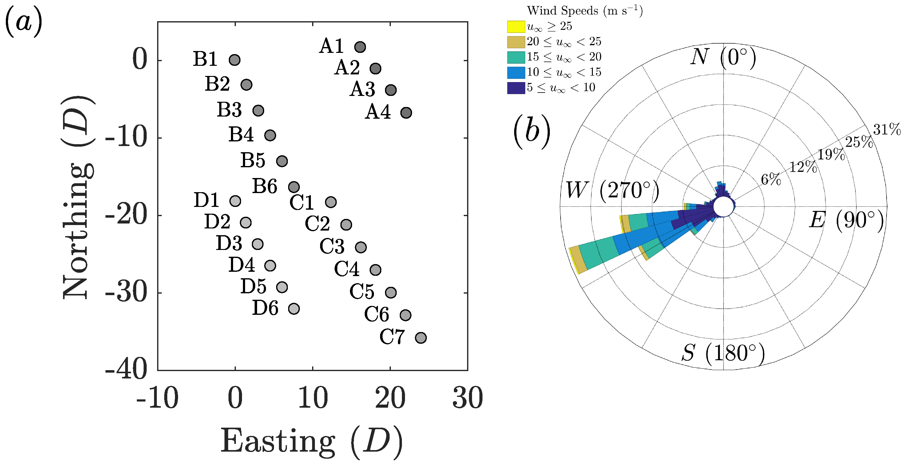
Five years of operational one-minute averaged SCADA data were used from a wind farm in Alberta, Canada. The wind farm consists of 23 irregularly spaced Vestas V80 turbines, as shown in Figure 3a. The wind farm layout was designed for predominantly high speed flow from the southwest at approximately 250° (Figure 3b). However, low speed flow from the northwest occurs during approximately of the nocturnal operation. Wind turbine spacing is approximately 10–15 turbine diameters for southwest flow while spacing is approximately 3–4 diameters for northwest flow. The model comparison focused on both the closely spaced 330° ± 5° inflow and the sparsely spaced 250° ± 5° inflow.
The wind inflow conditions were measured using nacelle mounted anemometers. Cup and sonic anemometers were used to measure the wind speed. The wind direction was measured using the nacelle direction, which was controlled to minimize the yaw misalignment angle measured between the nacelle direction and the nacelle mounted wind vane. The wind direction is prescribed by an average of the measurements of Turbines A1 and B1, which are in freestream conditions for the northwest and southwest flows. The wind speed model comparison conditional averaging is prescribed by Turbine B1. Model comparisons focused on wind turbine Columns A–D (Figure 3). The power production for the Summerview wind farm was taken from the SCADA data at a matched one-minute average instance for all wind turbines. Large wind farms have a advection time scale associated with the flow through time [66], which depends on the wind speed [67], but was neglected in this study. Some spatial discrepancies may occur due to the advection time within the wind farm [66], complex terrain [12], or mesoscale structures.
The Vestas V80 1.8 MW Turbine B1 power curve is shown in Figure 4. A reference manufacturer power curve is compared with the data. Time steps in which at least one turbine in Columns A–D is curtailed (defined here as producing at least 300 kW more or less than the power curve would suggest for a given wind speed) are removed from the dataset since the wake model would be corrupted due to the derating during such a circumstance. While the standard deviations in the power curve are small compared to the mean in Figure 4, the majority of the uncertainty within the dataset comes from noisy sensors and local discrepancies between wind turbines [68].
Each wind direction is split individually to ensure the quality of the data for each condition in each set. For 250° inflow, the number of examples are 12,286/13,027 in the training and development sets, respectively. For 330° inflow, the data split is 3462/3571.
3.2. Results
The various wake model architectures were trained and validated using the Summerview wind farm SCADA data. The influences of the initialization in the statistical models are discussed in Section 3.2.1. The various model architectures are compared in terms of MAE for 250° ± 5° inflow in Section 3.2.2 and for 330° ± 5° in Section 3.2.3. Finally, as presented in Section 3.2.4, the physics-based model was tested and key challenges with the physics approach were identified.
3.2.1. Initialization of Statistical Methods
The influence of the initialization method was tested for the nonlinearity method given by Equation (9) for inflow from 330°. The initialization of the weight matrices did not significantly influence the final training MAE shown in Table 2. This result is anticipated since there are enough trainable parameters to reproduce the mean power production with high accuracy. However, the Xavier initialized method does not generalize sufficiently in the present dataset to the development set shown in Table 2.
3.2.2. Influence of Architecture for 250° Inflow
The MAE for the training 250° dataset are shown for all architectures in Figure 5a. We can make a few main observations. The statistical models are all able to outperform the physics-based approach on the training set except for the nonlinear model. This is expected since the statistical models are not constrained by physics and have significantly more learnable parameters, allowing these models to produce the power production for which they are trained with high accuracy. In general, the two-layer neural network has the lowest training MAE since it has the largest set of trainable model parameters (see Table 1). The other statistical methods have similar training MAE values.
For the development dataset for 250° inflow (Figure 5b), differences arise between the various statistical methods. The linear method, nonlinear method, and two-layer neural networks perform similarly while the nonlinear method does not generalize to the development set. The linear method generalizes fairly well to the development set at different wind speeds. The physics-based method generally outperforms the statistical methods except for the deficit approaches.
The deficit approaches, both linear and nonlinear, reduce the development set MAE significantly when compared to the other statistical methods with the same number of tunable parameters. This result confirms that these shallow networks (one or two layers) are sensitive to local minima in training. Further, we can leverage a physics-informed architecture in order to improve model generalization and performance on the development dataset. The deficit architectures, both linear and nonlinear, reduce the development set MAE values by approximately a factor of two compared to the standard two-layer neural network in the –8 m/s case. The deficit architectures have less development MAE than the physics-based approach.
3.2.3. Influence of Architecture for 330° Inflow
The results are similar for the 330° inflow case. The MAE for the 330° inflow case is generally less than 250° since the wind speeds are lower from this direction (see Figure 3b), resulting in less power production. The deficit architectures have less development set MAE compared to the other statistical methods and the physics-based approach for the –15 m/s and –8 m/s cases. The errors for the physics-based lifting line model are relatively high for the 330° inflow case on the training set for –7 m/s. This is due to differences in the measured wind speed between the various turbines within the wind farm. In particular, there are differences between the wind speeds measured by Turbines A1, B1, and D1 which operate in freestream for 330° inflow. These differences among the turbines in freestream are less significant in the 250° inflow. This is likely due to the lower wind speeds where uncertainties in the wind speed measurements are more pronounced (see, e.g., [70]). As discussed in Section 3.2.4, the differences in freestream wind speeds between turbines are not captured in the present physics-based model architecture and should be included in future work.
In the present nonlinear network architecture (Equation (9)), the nonlinearity significantly outperformed the nonlinearity on the development datasets. In the present statistical models, the power production training data are not normalized or mean shifted, which is the standard practice in machine learning with neural networks [23]. Normalization and mean shifting significantly increased the final development MAE for the shallow networks considered in this study due to sensitivity to saddle points during training (not shown for brevity). As a result of the lack of mean shifting, the function likely saturates with development data for which the model was not trained. Since the method was designed specifically for the input range of the Vestas V80 power production, nonlinear activation saturation only occurs above the rated wind speed (see Figure 2).
3.2.4. Physics-Based Model
The physics-based lifting line model described in Section 2.1 has higher training and development dataset errors for the SCADA data for the Summerview wind farm than the data-driven approaches for some wind conditions. The physics-based lifting line model described in Section 2.1 is calibrated to the historical SCADA data for the Summerview wind farm in Alberta, Canada. The inflow wind speed is prescribed by Turbine D1 and the inflow wind direction is prescribed through an average of Turbines A1 and B1. The 250° inflow direction trained model power production is compared to the SCADA data and the linear model predictions for 250° ± 5° inflow in Figure 6a. As shown in Figure 3, for 250° inflow, Column D and parts of Columns B and C are in freestream inflow. This is represented in the model predictions where a significant number of turbines produce freestream power. However, in the SCADA data, several wind turbines that should produce freestream power levels through geometry are under-performing the power production of Turbine D1. This is likely due to the physics neglected in the lifting line model. In particular, there may be small topological differences within the wind farm which may cause local pressure gradients and wind acceleration [21] as well as mesoscale atmospheric structures [22] and operational discrepancies between the turbines. Since these physics were neglected in the development of the wake model, the wake model fit cannot capture these trends in power production. As a result, the physics-based wake model is constrained by the physics and cannot fully capture the power production. On the other hand, the statistical model is not constrained by a fixed inflow velocity measured at Turbine D1 and may fit the training data arbitrarily well given the number of trainable parameters.
For inflow from 330° ± 5°, the spacing between the wind turbines is small. For these wind directions, the physics-based model has lower MAE than the linear statistical method (Figure 5d) and the wake losses are well captured, as shown in Figure 6b, for –7 m/s in the development set. These data are model predictions since the physics-based model was not trained or tested for generalization on the validation dataset. The wake model shares the same parameters for all wind speeds which leads to power prediction error since wake losses are a function of the incoming wind speed. As a result, there are still some errors in the prediction of the wake losses.
Another key challenge in modeling the power production of a large wind farm is the inability for the static, time-averaged wake models to capture dynamic wake meandering (see, e.g., [63,71]) and wind gusts. The physics-based wake model assumes unidirectional, constant winds which is a coarse representation of the true ABL. The inflow direction of the unidirectional winds are prescribed by the nacelle positions of Turbines A1 and B1. However, this wind direction is subsequently used as the prescribed condition for Turbine C7 which is approximately 3.5 km away. Consider inflow from 330° for example. It is likely that the wakes of Column B turbines will merge into a large wind farm wake [16]. This wake is then subject to large-scale dynamic wake meandering which may cause it to directly impinge or miss Column C entirely. In the static wake model approach, these dynamics are averaged out and the Column B wakes would be represented as a fairly weak wake impinging upon Column C.
Finally, the present static model does not incorporate the influence of Coriolis forces which have been shown to play a role in the wakes of large wind farms in simulations [20] and field observations [16]. A basic model for the influence of Coriolis forces on the wakes of wind turbines was proposed by [13] but has not been validated in experimental studies and is left for future work.
4. Interpreting the Statistical Learning
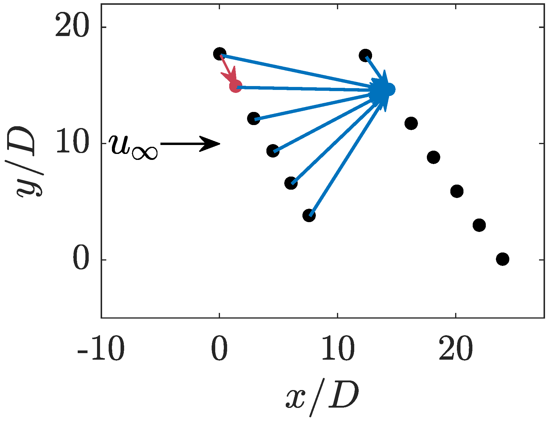
Machine learning has been applied to a wide variety of problems generally [23] and in fluid mechanics specifically (see, e.g., [24,25]); however, physical interpretability has generally been challenging. The present statistical methods are able to achieve low training and development MAE values for the present dataset, suggesting that the methods are potentially able to learn physically relevant statistically consistent relationships between the wind turbines. The statistical network is similar to a weighted directed acyclic graph for which a number of methods of visualization exist (see review by Herman et al. [72]). Presently, we visualize the connectivity through the magnitude and sign of the trained parameters (referred to hereafter as the dot plot). In particular, of Equation (7) is visualized for each downstream turbine with a fixed upstream turbine (black circle). The parameter is similar to a correlation in a regression model. The size of the circle describes the magnitude of and blue is a positive value while red is negative. The dot plot visualization method is used to qualitatively observe the learned methodology of the statistical learning used in this study. The focus of this visualization is the simple linear weight matrix in Equation (7) since shallow networks with fewer trainable parameters are generally more interpretable.
The dot plot visualization of the weight matrix is shown for 330° inflow for Turbine B1 in Figure 7a. Turbine B1 is the most upstream turbine so all downstream turbines have a connecting weight value . Further, Turbine B1 is a turbine which operates in freestream flow. Turbines A1 and C1 have a large weight connection to B1, likely because they are turbines also operating approximately in freestream flow. However, Turbine D1 is not significantly correlated. This could be due to topological differences or lateral variations between large-scale motions in the atmospheric boundary layer [73,74].
All turbines within the wake of Turbine D1 have similar values of , as shown in Figure 7b. These learned parameters are very similar to the assumptions of connectivity used by [47] in a wind farm network configuration.
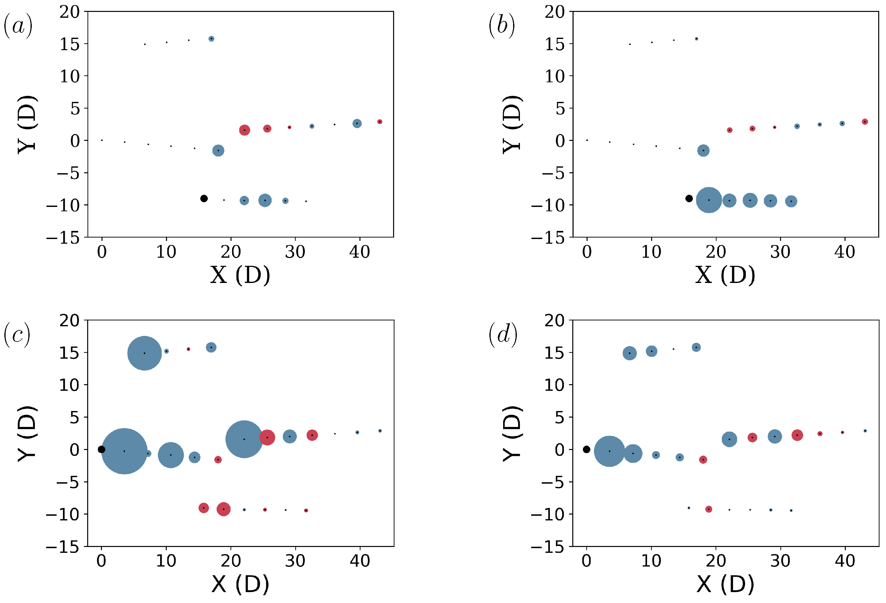
Influence of Statistical Learning Initialization
The initialization influenced the final trained parameters of the statistical wind farm model since shallow networks are subject to local minima. In this section, of Equation (9) is visualized for each downstream turbine with a fixed upstream turbine. This visualization is shown in Figure 8, where the Gaussian initialization is compared to the standard Xavier initialization [69]. The weight matrix correlations to Turbine D1 are visualized for the Xavier initialized model in Figure 8a and are difficult to interpret. On the other hand, the Gaussian initialized statistical method significantly correlates nearby turbines as well as turbines which are in the wake of Turbine D1 as shown in Figure 8b. Some wind turbine connectivity had reasonable qualitative agreement between the two initializations as shown in the correlation to Turbine B1 in Figure 8c,d.
Both initialization methods correlated the leading turbines of the columns (Columns A and C) with Turbine B1 (Figure 8c,d). The leading turbines of each column are operating in mostly freestream conditions as a result of the large spacing between the columns. Therefore, it is expected that leading, freestream turbines will have similar power production [47]. The dot plots confirm that the statistical methods may be learning physically relevant correlations and connections between wind turbines within the farm.
5. Conclusions
In the present paper, several novel statistical wake models are proposed to predict wind farm power production with the input of only the most upstream turbine power. These statistical methods were developed to overcome observed errors in wind farm power prediction by industry standard wake models, which occur as a result of model simplifications and assumptions. The statistical models were constructed to contain a similar number of trainable parameters to common industry wake models (e.g., Jensen model or Gaussian model [7]) in order to reduce overfitting to the training set. Additionally, reducing the number of training parameters increases the interpretability of the trained model constants. The most successful newly developed deficit-based data-driven network relies on physical information about the fluid dynamics of turbulent wind turbine wakes including Gaussian profiles for model initialization and power deficit for model architecture. Further, model nonlinearities are informed by the inherent nonlinearity in the wind turbine thrust as a function of the wind speed.
The deficit statistical models reduced the mean absolute error on the development dataset significantly compared to a standard two-layer neural network. The deficit statistical model reduced the development dataset mean absolute error compared to the standard linear weight matrix method with the same number of trainable parameters. This observation confirms that shallow statistical models are subject to local minima due to their low dimensionality and this may be mitigated through physics-informed statistical models.
The linear deficit wake model reduced the development dataset mean absolute error by and for the 250° and 330° inflow, respectively, compared to a physics-based low-order wake model. This success was due to the relaxation of physical constraints and model assumptions. Importantly, with the development dataset test protocol used in this study, the statistical and physical models can be compared with the same quantity of SCADA data inputs. While the physics-based model has advantages in control oriented approaches (see, e.g., [37,40,44,75]), statistical models reduce the power prediction error. Future work will consider how to incorporate controllability into the pure statistical approaches. Additionally, wind farm power forecasting errors remain a key issue in the integration of this low-carbon resource [76]. While weather variations account for the majority of forecasting challenges [77], wake losses contribute to the uncertainty. Future work will incorporate wind power forecast models with the newly developed statistical methods.
Author Contributions
M.F.H. and J.O.D. conceived the research; M.F.H. conducted analysis; and both authors wrote and edited the paper.
Funding
M.F.H. was funded through a National Science Foundation Graduate Research Fellowship under Grant No. DGE-1656518 and a Stanford Graduate Fellowship.
Acknowledgments
The authors would like to thank TransAlta Corporation and TransAlta Renewables for graciously providing historical wind farm operational data. The authors would also like to thank Valerie Troutman for assistance with the dot plot visualization method.
Conflicts of Interest
The authors declare no conflict of interest.
Abbreviations
The following abbreviations are used in this manuscript:
| A | Wind turbine rotor area |
| a | Axial induction factor |
| Learning rate | |
| ABL | Atmospheric boundary layer |
| Coefficient of power | |
| Coefficient of thrust | |
| Density | |
| D | Wind turbine diameter |
| DOAJ | Directory of open access journals |
| DoF | Degrees of freedom |
| Wake spreading coefficient | |
| MAE | Mean absolute error |
| MDPI | Multidisciplinary Digital Publishing Institute |
| Number of frontal wind turbines | |
| NN | Neural network |
| LL | Lifting line model |
| ReLU | Rectified linear unit |
| SCADA | Supervisory control and data acquisition |
| Gaussian wake proportionality constant | |
| based nonlinearity | |
| Sigmoid function | |
| Effective velocity | |
| Freestream velocity | |
| Lateral wake centroid |
Appendix A. Comparison of Linear Weight Matrix Method with Linear Ordinary Least Squares
The linear weight matrix method in Equation (7) is formally similar to linear ordinary least squares, which minimizes the sum of squared model residuals in the training dataset. For linear least squares, the power for a turbine i can be modeled as
where are weights. There is a unique solution for . This can be represented as a vector for each turbine i
where is a matrix of the power production of the turbines in front of turbine i and is a vector of power production for turbine i. While this method provides a unique solution to the minimization problem, ordinary least squares is not robust and generally produces errors in predicting conditional averages [55], which is particularly relevant to the wind farm modeling problem. Following the development set protocol (Section 2.4) for inflow from 330°, the ordinary least squares development set MAE for 0–15 m/s is 0.0737 MW. This is approximately an order of magnitude larger than the error of the deficit method (Figure 5).
Appendix B. Input–Output Training Example
An input–output pair from the training dataset is shown to demonstrate the utilization of the statistical model. The statistical methods introduced in Section 2 are used to demonstrate the model performance on the example from the training set. The flow considered is 250° ± 5°. The prediction of the SCADA power for Turbine C2 is considered. Turbine C2 is the 14th turbine downwind for this inflow direction. Therefore, there are 13 turbine power SCADA data points input into the model given by Equation (7) and 13 weight values ( where ). The nonlinear methods have two vectors of weight values each of length 13 ( and where ). The SCADA power inputs and weight values are shown in Table A1. The model predictions are 1.467 MW, 1.432 MW, 1.528 MW, 1.483 MW, and 1.533 MW for the linear, linear deficit, nonlinear, nonlinear deficit, and architectures, respectively. The SCADA power production is 1.461 MW.

Table A1.
Input–output training example for the various statistical models proposed in Section 2. One one-minute averaged data training example is shown. The inflow is from 250° ± 5°. The turbine of interest is C2, which is the 14th turbine downwind for inflow from this direction.
Table A1.
Input–output training example for the various statistical models proposed in Section 2. One one-minute averaged data training example is shown. The inflow is from 250° ± 5°. The turbine of interest is C2, which is the 14th turbine downwind for inflow from this direction.
| Turbine | D1 | D2 | D3 | D4 | D5 | D6 | B1 | B2 | B3 | B4 | B5 | B6 | C1 |
|---|---|---|---|---|---|---|---|---|---|---|---|---|---|
| Power (MW) | 1.80 | 1.80 | 1.80 | 1.80 | 1.80 | 1.80 | 1.64 | 1.64 | 1.80 | 1.78 | 1.80 | 1.27 | 1.29 |
| Linear, | 0.279 | 0.014 | 0.129 | 0.014 | 0.087 | 0.085 | 0.262 | 0.423 | |||||
| Linear deficit, | 0.781 | 0.604 | 1.272 | 1.416 | 0.066 | 0.167 | 0.809 | 1.090 | 0.034 | ||||
| , | 0.257 | 0.629 | 0.146 | 0.122 | 0.056 | 0.375 | 0.181 | 0.746 | 0.648 | ||||
| , | 0.117 | 0.533 | 0.203 | 0.025 | 0.161 | 0.176 | 0.575 | 0.803 | |||||
| deficit, | 0.268 | 0.670 | 2.667 | 0.140 | 0.282 | 0.822 | 0.977 | ||||||
| deficit, | 0.574 | 1.470 | 0.814 | 0.207 | 0.132 | 0.708 | 1.055 | ||||||
| , | 0.128 | 0.367 | 0.380 | 0.023 | 0.177 | 0.195 | 0.496 | 0.503 | |||||
| , | 0.252 | 0.325 | 0.093 | 0.211 | 0.438 | 0.397 | 0.025 | 0.487 | 0.482 |
References
- IPCC. Global Warming of 1.5 ∘C: An IPCC Special Report on the Impacts of Global Warming of 1.5 ∘C above Pre-Industrial Levels and Related Global Greenhouse Gas Emission Pathways, in the Context of Strengthening the Global Response to the Threat of Climate Change, Sustainable Development, and Efforts to Eradicate Poverty; IPCC: Geneva, Switzerland, 2018. [Google Scholar]
- Moné, C.; Hand, M.; Bolinger, M.; Rand, J.; Heimiller, D.; Ho, J. 2015 Cost of Wind Energy Review; Technical Report; National Renewable Energy Lab. (NREL): Golden, CO, USA, 2017.
- Stevens, R.J.; Hobbs, B.F.; Ramos, A.; Meneveau, C. Combining economic and fluid dynamic models to determine the optimal spacing in very large wind farms. Wind Energy 2017, 20, 465–477. [Google Scholar] [CrossRef]
- Barthelmie, R.J.; Hansen, K.; Frandsen, S.T.; Rathmann, O.; Schepers, J.; Schlez, W.; Phillips, J.; Rados, K.; Zervos, A.; Politis, E.; et al. Modelling and measuring flow and wind turbine wakes in large wind farms offshore. Wind Energy 2009, 12, 431–444. [Google Scholar] [CrossRef]
- Crespo, A.; Hernandez, J.; Frandsen, S. Survey of modelling methods for wind turbine wakes and wind farms. Wind Energy 1999, 2, 1–24. [Google Scholar] [CrossRef]
- Stevens, R.J.; Meneveau, C. Flow structure and turbulence in wind farms. Ann. Rev. Fluid Mech. 2017, 49, 311–339. [Google Scholar] [CrossRef]
- Bastankhah, M.; Porté-Agel, F. A new analytical model for wind-turbine wakes. Renew. Energy 2014, 70, 116–123. [Google Scholar] [CrossRef]
- Shapiro, C.R.; Gayme, D.F.; Meneveau, C. Modelling yawed wind turbine wakes: A lifting line approach. J. Fluid Mech. 2018, 841, R1. [Google Scholar] [CrossRef]
- Annoni, J.; Fleming, P.; Scholbrock, A.; Roadman, J.; Dana, S.; Adcock, C.; Porte-Agel, F.; Raach, S.; Haizmann, F.; Schlipf, D. Analysis of Control-Oriented Wake Modeling Tools Using Lidar Field Results; Technical Report; National Renewable Energy Lab. (NREL): Golden, CO, USA, 2018.
- Meneveau, C. Big wind power: Seven questions for turbulence research. J. Turbul. 2019, 20, 2–20. [Google Scholar] [CrossRef]
- Stevens, R.J.; Gayme, D.F.; Meneveau, C. Coupled wake boundary layer model of wind-farms. J. Renew. Sustain. Energy 2015, 7, 023115. [Google Scholar] [CrossRef] [Green Version]
- Politis, E.S.; Prospathopoulos, J.; Cabezon, D.; Hansen, K.S.; Chaviaropoulos, P.; Barthelmie, R.J. Modeling wake effects in large wind farms in complex terrain: The problem, the methods and the issues. Wind Energy 2012, 15, 161–182. [Google Scholar] [CrossRef]
- Howland, M.F.; Ghate, A.S.; Lele, S.K. Influence of the horizontal component of Earth’s rotation on wind turbine wakes. In Journal of Physics: Conference Series; IOP Publishing: Bristol, UK, 2018; Volume 1037, p. 072003. [Google Scholar]
- Schlez, W.; Neubert, A. New developments in large wind farm modelling. In Proceedings of the European Wind Energy Conference, Marseilles, France, 16–19 March 2009. [Google Scholar]
- Johnson, C.; Graves, A.; Tindal, A.; Cox, S.; Schlez, W.; Neubert, A. New developments in wake models for large wind farms. In AWEA Windpower Conference; Garrad Hassan America Inc.: Chicago, IL, USA, 2009. [Google Scholar]
- Nygaard, N.G.; Newcombe, A.C. Wake behind an offshore wind farm observed with dual-Doppler radars. In Journal of Physics: Conference Series; IOP Publishing: Bristol, UK, 2018; Volume 1037, p. 072008. [Google Scholar]
- Nygaard, N.G. Wakes in very large wind farms. In Journal of Physics: Conference Series; IOP Publishing: Bristol, UK, 2014; Volume 524, p. 012162. [Google Scholar]
- Platis, A. First in situ evidence of wakes in the far field behind offshore wind farms. Sci. Rep. 2018, 8, 2163. [Google Scholar] [CrossRef] [PubMed]
- Lundquist, J.; DuVivier, K.; Kaffine, D.; Tomaszewski, J. Costs and consequences of wind turbine wake effects arising from uncoordinated wind energy development. Nat. Energy 2019, 4, 26. [Google Scholar] [CrossRef]
- Van der Laan, M.; Hansen, K.S.; Sørensen, N.N.; Réthoré, P.E. Predicting wind farm wake interaction with RANS: An investigation of the Coriolis force. In Journal of Physics: Conference Series; IOP Publishing: Bristol, UK, 2015; Volume 625, p. 012026. [Google Scholar]
- Yang, X.; Pakula, M.; Sotiropoulos, F. Large-eddy simulation of a utility-scale wind farm in complex terrain. Appl. Energy 2018, 229, 767–777. [Google Scholar] [CrossRef]
- Sanz Rodrigo, J.; Chavez Arroyo, R.A.; Moriarty, P.; Churchfield, M.; Kosović, B.; Réthoré, P.E.; Hansen, K.S.; Hahmann, A.; Mirocha, J.D.; Rife, D. Mesoscale to microscale wind farm flow modeling and evaluation. Wiley Interdiscip. Rev. Energy Environ. 2017, 6, e214. [Google Scholar] [CrossRef]
- LeCun, Y.; Bengio, Y.; Hinton, G. Deep learning. Nature 2015, 521, 436. [Google Scholar] [CrossRef] [PubMed]
- Cardona, J.L.; Howland, M.F.; Dabiri, J.O. Seeing the Wind: Visual Wind Speed Prediction with a Coupled Convolutional and Recurrent Neural Network. arXiv 2019, arXiv:1905.13290. [Google Scholar]
- Ling, J.; Kurzawski, A.; Templeton, J. Reynolds averaged turbulence modelling using deep neural networks with embedded invariance. J. Fluid Mech. 2016, 807, 155–166. [Google Scholar] [CrossRef]
- Kutz, J.N. Deep learning in fluid dynamics. J. Fluid Mech. 2017, 814, 1–4. [Google Scholar] [CrossRef] [Green Version]
- Park, J.; Law, K.H. Bayesian ascent: A data-driven optimization scheme for real-time control with application to wind farm power maximization. IEEE Trans. Control Syst. Technol. 2016, 24, 1655–1668. [Google Scholar] [CrossRef]
- Park, J.; Law, K.H. A data-driven, cooperative wind farm control to maximize the total power production. Appl. Energy 2016, 165, 151–165. [Google Scholar] [CrossRef]
- Lei, M.; Shiyan, L.; Chuanwen, J.; Hongling, L.; Yan, Z. A review on the forecasting of wind speed and generated power. Renew. Sustain. Energy Rev. 2009, 13, 915–920. [Google Scholar] [CrossRef]
- Wan, C.; Xu, Z.; Pinson, P.; Dong, Z.Y.; Wong, K.P. Probabilistic forecasting of wind power generation using extreme learning machine. IEEE Trans. Power Syst. 2014, 29, 1033–1044. [Google Scholar] [CrossRef]
- Haque, A.U.; Mandal, P.; Meng, J.; Negnevitsky, M. Wind speed forecast model for wind farm based on a hybrid machine learning algorithm. Int. J. Sustain. Energy 2015, 34, 38–51. [Google Scholar] [CrossRef]
- González, J.S.; Rodriguez, A.G.G.; Mora, J.C.; Santos, J.R.; Payan, M.B. Optimization of wind farm turbines layout using an evolutive algorithm. Renew. Energy 2010, 35, 1671–1681. [Google Scholar] [CrossRef]
- Thomas, J.J.; Annoni, J.; Fleming, P.A.; Ning, A. Comparison of Wind Farm Layout Optimization Results Using a Simple Wake Model and Gradient-Based Optimization to Large Eddy Simulations. In Proceedings of the AIAA Scitech 2019 Forum, San Diego, CA, USA, 7–11 January 2019; p. 0538. [Google Scholar]
- Fleming, P.A.; Ning, A.; Gebraad, P.M.; Dykes, K. Wind plant system engineering through optimization of layout and yaw control. Wind Energy 2016, 19, 329–344. [Google Scholar] [CrossRef]
- Fleming, P.; Annoni, J.; Shah, J.J.; Wang, L.; Ananthan, S.; Zhang, Z.; Hutchings, K.; Wang, P.; Chen, W.; Chen, L. Field test of wake steering at an offshore wind farm. Wind Energy Sci. 2017, 2, 229–239. [Google Scholar] [CrossRef] [Green Version]
- Bay, C.J.; Annoni, J.; Taylor, T.; Pao, L.; Johnson, K. Active power control for wind farms using distributed model predictive control and nearest neighbor communication. In Proceedings of the 2018 Annual American Control Conference (ACC), Milwaukee, WI, USA, 27–29 June 2018; pp. 682–687. [Google Scholar]
- Fleming, P.; King, J.R.; Dykes, K.L.; Simley, E.J.; Roadman, J.M.; Scholbrock, A.K.; Murphy, P.; Lundquist, J.K.; Moriarty, P.J.; Fleming, K.A.; et al. Initial Results From a Field Campaign of Wake Steering Applied at a Commercial Wind Farm: Part 1; Technical Report; National Renewable Energy Lab. (NREL): Golden, CO, USA, 2019.
- Moin, P.; Mahesh, K. Direct numerical simulation: A tool in turbulence research. Ann. Rev. Fluid Mech. 1998, 30, 539–578. [Google Scholar] [CrossRef]
- Gebraad, P.; Teeuwisse, F.; Wingerden, J.; Fleming, P.A.; Ruben, S.; Marden, J.; Pao, L. Wind plant power optimization through yaw control using a parametric model for wake effects—A CFD simulation study. Wind Energy 2016, 19, 95–114. [Google Scholar] [CrossRef]
- Boersma, S.; Doekemeijer, B.; Gebraad, P.M.; Fleming, P.A.; Annoni, J.; Scholbrock, A.K.; Frederik, J.; van Wingerden, J.W. A tutorial on control-oriented modeling and control of wind farms. In Proceedings of the 2017 American Control Conference (ACC), Seattle, WA, USA, 24–26 May 2017; pp. 1–18. [Google Scholar]
- Bhaskar, K.; Singh, S. AWNN-assisted wind power forecasting using feed-forward neural network. IEEE Trans. Sustain. Energy 2012, 3, 306–315. [Google Scholar] [CrossRef]
- Gebraad, P.M.; Van Wingerden, J. A control-oriented dynamic model for wakes in wind plants. In Journal of Physics: Conference Series; IOP Publishing: Bristol, UK, 2014; Volume 524, p. 012186. [Google Scholar]
- Shapiro, C.R.; Bauweraerts, P.; Meyers, J.; Meneveau, C.; Gayme, D.F. Model-based receding horizon control of wind farms for secondary frequency regulation. Wind Energy 2017, 20, 1261–1275. [Google Scholar] [CrossRef]
- Howland, M.F.; Lele, S.K.; Dabiri, J.O. Wind farm power optimization through wake steering. Proc. Natl. Acad. Sci. USA 2019, 201903680. [Google Scholar] [CrossRef]
- Doekemeijer, B.M.; Boersma, S.; Pao, L.Y.; Knudsen, T.; van Wingerden, J.W. Online model calibration for a simplified LES model in pursuit of real-time closed-loop wind farm control. Wind Energy Sci. Discuss. 2018, 2018, 1–30. [Google Scholar] [CrossRef]
- Burton, T.; Jenkins, N.; Sharpe, D.; Bossanyi, E. Wind Energy Handbook; John Wiley & Sons: Hoboken, NJ, USA, 2011. [Google Scholar]
- Annoni, J.; Bay, C.; Taylor, T.; Pao, L.; Fleming, P.; Johnson, K. Efficient Optimization of Large Wind Farms for Real-Time Control. In Proceedings of the 2018 Annual American Control Conference (ACC), Milwaukee, WI, USA, 27–29 June 2018; pp. 6200–6205. [Google Scholar]
- Katic, I.; Højstrup, J.; Jensen, N.O. A simple model for cluster efficiency. In Proceedings of the European Wind Energy Association Conference and Exhibition, Rome, Italy, 7–9 October 1986. [Google Scholar]
- Meyers, J.; Meneveau, C. Optimal turbine spacing in fully developed wind farm boundary layers. Wind Energy 2012, 15, 305–317. [Google Scholar] [CrossRef]
- Kingma, D.P.; Ba, J. Adam: A method for stochastic optimization. arXiv 2014, arXiv:1412.6980. [Google Scholar]
- Hansen, K.S.; Réthoré, P.E.; Palma, J.; Hevia, B.; Prospathopoulos, J.; Peña, A.; Ott, S.; Schepers, G.; Palomares, A.; Van der Laan, M.; et al. Simulation of wake effects between two wind farms. In Journal of Physics: Conference Series; IOP Publishing: Bristol, UK, 2015; Volume 625, p. 012008. [Google Scholar]
- Hutchins, N.; Marusic, I. Evidence of very long meandering features in the logarithmic region of turbulent boundary layers. J. Fluid Mech. 2007, 579, 1–28. [Google Scholar] [CrossRef] [Green Version]
- Howland, M.; Yang, X. Dependence of small-scale energetics on large scales in turbulent flows. J. Fluid Mech. 2018, 852, 641–662. [Google Scholar] [CrossRef] [Green Version]
- Kochenderfer, M.J. Decision Making under Uncertainty: Theory and Application; MIT Press: Cambridge, MA, USA, 2015. [Google Scholar]
- Koenker, R.; Hallock, K.F. Quantile regression. J. Econ. Perspect. 2001, 15, 143–156. [Google Scholar] [CrossRef]
- Milan, P.; Wächter, M.; Peinke, J. Turbulent character of wind energy. Phys. Rev. Lett. 2013, 110, 138701. [Google Scholar] [CrossRef]
- Bossuyt, J.; Howland, M.F.; Meneveau, C.; Meyers, J. Measurement of unsteady loading and power output variability in a micro wind farm model in a wind tunnel. Exp. Fluids 2017, 58, 1. [Google Scholar] [CrossRef]
- Nguyen, D.; Widrow, B. Improving the learning speed of 2-layer neural networks by choosing initial values of the adaptive weights. In Proceedings of the 1990 IJCNN International Joint Conference on Neural Networks, San Diego, CA, USA, 17–21 June 1990; pp. 21–26. [Google Scholar]
- Göçmen, T.; Van der Laan, P.; Réthoré, P.E.; Diaz, A.P.; Larsen, G.C.; Ott, S. Wind turbine wake models developed at the technical university of Denmark: A review. Renew. Sustain. Energy Rev. 2016, 60, 752–769. [Google Scholar] [CrossRef] [Green Version]
- Paszke, A.; Gross, S.; Chintala, S.; Chanan, G.; Yang, E.; DeVito, Z.; Lin, Z.; Desmaison, A.; Antiga, L.; Lerer, A. Automatic differentiation in pytorch. In Proceedings of the 31st Conference on Neural Information Processing Systems (NIPS 2017), Long Beach, CA, USA, 4–9 December 2017. [Google Scholar]
- Sutskever, I.; Martens, J.; Dahl, G.; Hinton, G. On the importance of initialization and momentum in deep learning. In Proceedings of the International conference on machine learning, Atlanta, GA, USA, 16–21 June 2013; pp. 1139–1147. [Google Scholar]
- Chamorro, L.P.; Porté-Agel, F. Effects of thermal stability and incoming boundary-layer flow characteristics on wind-turbine wakes: A wind-tunnel study. Bound. Layer Meteorol. 2010, 136, 515–533. [Google Scholar] [CrossRef]
- Larsen, T.J.; Madsen, H.A.; Larsen, G.C.; Hansen, K.S. Validation of the dynamic wake meander model for loads and power production in the Egmond aan Zee wind farm. Wind Energy 2013, 16, 605–624. [Google Scholar] [CrossRef]
- Niayifar, A.; Porté-Agel, F.; Porté-Agel, F.A. A new analytical model for wind farm power prediction. In Journal of Physics: Conference Series; IOP Publishing: Bristol, UK, 2015; Volume 625, p. 012039. [Google Scholar]
- Krizhevsky, A.; Hinton, G. Convolutional deep belief networks on cifar-10. Unpubl. Manuscr. 2010, 40, 1–9. [Google Scholar]
- Lukassen, L.J.; Stevens, R.J.; Meneveau, C.; Wilczek, M. Modeling space-time correlations of velocity fluctuations in wind farms. Wind Energy 2018, 21, 474–487. [Google Scholar] [CrossRef] [Green Version]
- Yang, X.; Howland, M. Implication of Taylor’s hypothesis on measuring flow modulation. J. Fluid Mech. 2018, 836, 222–237. [Google Scholar] [CrossRef]
- Annoni, J.; Bay, C.; Johnson, K.; Dall’Anese, E.; Quon, E.; Kemper, T.; Fleming, P. A Framework for Autonomous Wind Farms: Wind Direction Consensus. Wind Energy Sci. 2019, 4, 355–368. [Google Scholar] [CrossRef]
- Glorot, X.; Bengio, Y. Understanding the difficulty of training deep feedforward neural networks. In Proceedings of the thirteenth international conference on artificial intelligence and statistics, Sardinia, Italy, 13–15 May 2010; pp. 249–256. [Google Scholar]
- Murcia, J.P.; Réthoré, P.E.; Hansen, K.S.; Natarajan, A.; Sørensen, J.D. A new method to estimate the uncertainty of AEP of offshore wind power plants applied to Horns Rev 1. In EWEA Annual Conference and Exhibition 2015; European Wind Energy Association (EWEA): Brussels, Belgium, 2015. [Google Scholar]
- Medici, D.; Alfredsson, P.H. Measurements behind model wind turbines: Further evidence of wake meandering. Wind Energy 2008, 11, 211–217. [Google Scholar] [CrossRef]
- Herman, I.; Melançon, G.; Marshall, M.S. Graph visualization and navigation in information visualization: A survey. IEEE Trans. Vis. Comput. Graph. 2000, 6, 24–43. [Google Scholar] [CrossRef] [Green Version]
- Marusic, I.; Mathis, R.; Hutchins, N. Predictive model for wall-bounded turbulent flow. Science 2010, 329, 193–196. [Google Scholar] [CrossRef] [PubMed]
- Katul, G. The anatomy of large-scale motion in atmospheric boundary layers. J. Fluid Mech. 2019, 858, 1–4. [Google Scholar] [CrossRef]
- Martínez-Tossas, L.A.; Annoni, J.; Fleming, P.A.; Churchfield, M.J. The aerodynamics of the curled wake: A simplified model in view of flow control. Wind Energy Sci. 2019, 4, 127–138. [Google Scholar] [CrossRef]
- Gu, Y.; McCalley, J.D.; Ni, M. Coordinating large-scale wind integration and transmission planning. IEEE Trans. Sustain. Energy 2012, 3, 652–659. [Google Scholar] [CrossRef]
- Sideratos, G.; Hatziargyriou, N.D. An advanced statistical method for wind power forecasting. IEEE Trans. Power Syst. 2007, 22, 258–265. [Google Scholar] [CrossRef]
Figure 1.
Diagram of the statistical model architecture. The dots represent wind turbines with flow from left to right. The power production of all upstream turbines are used for the power prediction of a given downstream turbine. The red arrows denote the weighted connection of the upstream turbine to the downstream red turbine. The blue arrows denote the weighted connection of the upstream turbines to the downstream blue turbine.

Figure 2.
(a) Vestas V80 manufacturer rated coefficient of thrust curve () compared with the Sigmoid-type activation function , which is based on the inherent wake strength nonlinearity caused by the wind turbine curve. The activation function is given by Equation (8). (b) Nonlinearities applied to the Vestas V80 power curve. The sigmoid-type activation function is . The nonlinearity was designed such that followed .

Figure 3.
(a) Summerview wind farm in Alberta, Canada oriented with the cardinal directions, viewed from above. The circles have a diameter of approximately D. Turbines within each column are numbered north to south. (b) Wind rose for the Summerview wind farm measured by Turbine B1.
Figure 3.
(a) Summerview wind farm in Alberta, Canada oriented with the cardinal directions, viewed from above. The circles have a diameter of approximately D. Turbines within each column are numbered north to south. (b) Wind rose for the Summerview wind farm measured by Turbine B1.

Figure 4.
Power curve for a Vestas V80 turbine at the Summerview wind farm in Alberta, Canada for 250° inflow. The raw one-minute averaged data are shown with dots. Averaged data in 0.25 m/s bins are shown in red. The error bars represent one standard deviation in the data and are assumed to be symmetric about the mean. Horizontal error bars of ±0.25 m/s are not included in the figure. is a reference manufacturer power curve.

Figure 5.
(a,b) Mean absolute errors for the various low-order model architectures for the (a) training and (b) development datasets for 250° inflow. (c,d) Mean absolute errors for the various low-order model architectures for the (c) training and (d) development datasets for 330° inflow.
Figure 5.
(a,b) Mean absolute errors for the various low-order model architectures for the (a) training and (b) development datasets for 250° inflow. (c,d) Mean absolute errors for the various low-order model architectures for the (c) training and (d) development datasets for 330° inflow.

Figure 6.
Average power production as a function of turbine number for the lifting line model and linear weight matrix method in Equation (7) for inflow from (a) 250° ± 5° training data for all wind speeds and (b) 330° ± 5° development data for –7 m/s. Turbines are numbered following Columns A–D. Turbine 8 is a 2 MW machine while the rest are 1.8 MW.

Figure 7.
(a) Weight matrix in Equation (7) visualization for inflow from 330° ± 5° the linear statistical method. The value of the weight matrices for downstream turbines is plotted with respect to the black dot upstream Turbine B1. The size of the circle represents the magnitude of the weight matrix value and blue represents positive while red is negative. (b) Same as (a) with the upstream turbine of D1.

Figure 8.
Weight matrix visualization for the nonlinearity method with (a) Xavier [69] and (b) Gaussian initialization for Turbine D1 and (c) Xavier and (d) Gaussian for Turbine B1. For the nonlinearity method in Equation (9), is visualized. The value of the weight matrices for downstream turbines is plotted with respect to the black dot upstream turbine. The size of the circle represents the magnitude of the weight matrix value and blue represents positive while red is negative.

Table 1.
Learnable parameters and their associated degrees of freedom (DoF) for the statistical models used in the present study. The degree of freedom is given for the prediction of a single arbitrary turbine within the wind farm with turbines in front. The linear and nonlinear learnable parameters apply to the deficit and standard methods.
| Method | Parameter | DoF |
|---|---|---|
| Linear | w | |
| Nonlinear | k | |
| c | ||
| Neural network | ||
| 1 |
Table 2.
Comparison of initialization methods for the statistical learning model for inflow from 330 ± 5° for all wind speeds in the dataset. The statistical learning model is initialized with the Xavier [69] and the Gaussian (Equation (13)) approaches.
| Method | MAE Train (MW) | MAE Dev (MW) |
|---|---|---|
| Xavier | 0.005 | 0.032 |
| Gaussian | 0.005 | 0.020 |
© 2019 by the authors. Licensee MDPI, Basel, Switzerland. This article is an open access article distributed under the terms and conditions of the Creative Commons Attribution (CC BY) license (http://creativecommons.org/licenses/by/4.0/).
Share and Cite
MDPI and ACS Style
Howland, M.F.; Dabiri, J.O. Wind Farm Modeling with Interpretable Physics-Informed Machine Learning. Energies 2019, 12, 2716. https://doi.org/10.3390/en12142716
AMA Style
Howland MF, Dabiri JO. Wind Farm Modeling with Interpretable Physics-Informed Machine Learning. Energies. 2019; 12(14):2716. https://doi.org/10.3390/en12142716
Chicago/Turabian StyleHowland, Michael F., and John O. Dabiri. 2019. "Wind Farm Modeling with Interpretable Physics-Informed Machine Learning" Energies 12, no. 14: 2716. https://doi.org/10.3390/en12142716
Note that from the first issue of 2016, this journal uses article numbers instead of page numbers. See further details here.