Steady Flow of a Cement Slurry


1
U. S. Department of Energy, National Energy Technology Laboratory (NETL), Pittsburgh, PA 15236, USA
2
School of Mechanical Engineering, Nanjing University of Science and Technology, Nanjing 210094, China
*
Author to whom correspondence should be addressed.
Energies 2019, 12(13), 2604; https://doi.org/10.3390/en12132604
Submission received: 12 June 2019
/
Revised: 3 July 2019
/
Accepted: 5 July 2019
/
Published: 6 July 2019
(This article belongs to the Special Issue Mathematical Modeling of Fluid Flow and Heat Transfer in Petroleum Industries and Geothermal Applications)
Abstract
:Understanding the rheological behavior of cement slurries is important in cement and petroleum industries. In this paper, we study the fully developed flow of a cement slurry inside a wellbore. The slurry is modeled as a non-linear fluid, where a constitutive relation for the viscous stress tensor based on a modified form of the second grade (Rivlin–Ericksen) fluid is used;we also propose a diffusion flux vector for the concentration of particles. The one-dimensional forms of the governing equations and the boundary conditions are made dimensionless and solved numerically. A parametric study is performed to present the effect of various dimensionless numbers on the velocity and the volume fraction profiles.
1. Introduction
Portland cement is widely used as a construction material in civil engineering applications due to the widespread availability of its constituent materials [1]. It is produced from the grinding of clinker, which is produced by the calcination of limestone and other raw materials in a rotary kiln. The different phases in cement are: Alite (C3S), belite (C2S), aluminate phase (C3A), ferrite phase (C3AF), alkali sulfate, free lime, and gypsum [2,3]. Cement slurries are reactive systems, continuously changing their chemical and physical characteristics [4]. After the cement is mixed with water, a series of exothermal chemical reactions occur resulting in an increase in the strength and hardening [5]. The most reactive phases with water are C3S and C3A, the content of which affect the strength of cement developed at early stages. Water to cement ratio, which is defined as the ratio of the weight of water to the weight of cement, also plays an important role in the strength development and flow behavior of cement slurry.
According to a recent study by the United States Geological Survey (USGS), U.S. cement and clinker production is about 80 million metric tons per year. The production of cementitious materials consumes a significant amount of energy (20–40% total energy cost) [6,7]. Cement production also contributes to 4% of the global industrial carbon dioxide (CO2) emissions [8]. Therefore, it is important for the cement industry to seek energy efficient technologies and improve the performance of cement productions for sustainability purpose. Physical testing is widely applied to study the cement behavior. This requires time, energy, and material resources. In the past few decades, the cement research community has sought advanced computational modeling for cement hydration processes, flow and mechanical properties in order to eliminate the substantial cost for physical testing of cement. Bentz [9] developed a three-dimensional computational model for the cement microstructure and cement hydration process. Haekck et al. [10] studied the physical and the chemical properties of cement such as the heat of hydration, the elastic modulus, and the pore concentrations using the software Virtual Cement and Concrete Testing Laboratory (VCCTL). Bullard et al. described the details of this software [11,12]. Watts et al. [13] and Tao et al. [14] validated the software optimization framework to characterize and evaluate different computational models for cement.
In petroleum-related applications, cement slurries are pumped down the wellbore and up the annular space between the casing and the geological formations surrounding the wellbore to provide zonal isolation in oil, gas, and water wells [15]. It is a great challenge for petroleum industry to prevent gas entry into the cement and achieve the annular cement seal for a long term [16]. Researchers have investigated the possible mechanisms for fluid migration during cementing by using experimental and computational models, although the exact failure mechanism of this problem is very complicated. Monitoring the conditions of cement slurry in realtime is a critical issue where wireless sensor network-based monitoring system can be used [17]. Cement must remain as a fluid long enough while it is being pumped to the anticipated location; it should also have sound compressive-strength within a specific time after placement. Gel strength is related to the resisting shear stress before the cement can flow, and is considered to be one of the major factors for hydrostatic pressure loss and gas migration [18]. Chenevert and Jin [19] suggested that the rheological properties of the cement affect the static gel strength. Stiles [20] indicated that the rheological properties of the cement slurry are related to the annular fluid displacement. Brandt et al. [21] investigated a deep-water operation for drilling fluid and well cementing, and suggested that the slurry properties at low temperatures and high pressures should be taken into consideration. During the cementing, when the slurry is pumped into the oilwell, it flows to the bottom of the wellbore through the casing and begins to develop more strength from sedimentation. To develop computational models for cement slurry, many researchers assume that the cement slurry is a suspension with non-Newtonian characteristics [22]. Foroushan et al. [23] modeled the instability of the interface and the mixing of cement slurry and drilling mud during cementing operation in oil and gas wells in three dimensions by using commercial Computational Fluid Dynamics (CFD) software, and compared the results with experiments. Skadsem et al. [24] studied the flow of a non-Newtonian fluid in an inclined wellbore with concentric and eccentric configurations numerically and experimentally, using a finite element approach in OpenFOAM. Liu et al. [25] modeled the multi-phase pipe flow and considered the hydration effect of cemented paste backfill slurry by applying a CFD model. Murphy et al. [26] simulated the shear flow of two Bingham-type plastic cement slurries containing Portland cement and fly ash particles by applying the fast lubrication dynamics and discrete element model with LAMMPS.
In this paper, the flow of a cement slurry between two flat plates at different tilt angles is studied. It is assumed that the viscosity of the cement depends on the shear rate and the volume fraction of the particles. A convection–diffusion equation is used to study the effect of the particle concentration. Section 2 presents the governing equations. In Section 3, we describe the constitutive relations for the viscous stress and the diffusive particle flux vector. Section 4 defines the geometry of the problem and provides the dimensionless forms of the equations and the boundary conditions. In Section 5, numerical results are presented, and a parametric study is performed for different dimensionless numbers. Section 6 provides some concluding remarks.
2. Governing Equations
In this paper, cement slurry is assumed to behave as a non-homogenous nonlinear suspension. If the electromagnetic and the thermochemical effects are ignored, then the governing equations of motion are the conservations of mass, linear momentum, angular momentum, and the equation for the flux of concentration [27].
2.1. Conservation of Mass
2.2. Conservation of Linear Momentum
2.3. Conservation of Angular Momentum
The conservation of angular momentum indicates that in the absence of couple stresses the stress tensor is symmetric, that is
2.4. Convection–Diffusion Equation
In flows of suspensions, a convection–diffusion equation [28] is often used for the particle concentration
where is the rate of accumulation of particles, is the term representing particle migration and movement due to the flow, and is the diffusive particle flux. The function , called the volume fraction (related to concentration), has the property . In reality, is either one or zero at any position and time, depending upon whether one is pointing to a particle or to the void space (fluid) at that location. The density of the cement slurry, in general, can be related to the density of water and the cement particles, via the following relation: , where is the volume fraction (concentration) of the cement particles, and are the pure density of water and the cement particles in the reference configuration (before mixing), respectively. The assumption that the particle and the fluid densities are the same, is a special case of the above equation. In this paper, we use as the bulk density of the cement slurry.
Looking at Equations (1)–(4), we can see that we need constitutive relations for and . We will discuss these in the next section.
3. Constitutive Relations
A cement slurry, in general, behaves as a (nonlinear) fluid. Once cement particles are mixed with water, after a series of hydration reactions, the slurry begins to develop solidlike behavior [29]. Cement-based materials could stand under their own weight without flowing and develop strength and stiffness during setting [30]. The flow behavior of slurry plays an important role on the cement quality [31]. Understanding the rheological behavior of a cement slurry is important in industry for easy pumping and filling the annulus without excessive separation of water and cement [15,30]. Rheological measurements for cement-based materials are well established [32]. The Bingham viscoplastic fluid model is widely used to describe the yield stress of cement slurries. The yield stress is often related to particle concentration, shear rate history, time, and temperature. The static yield stress (also known as the static gel strength) affects the pumping of the cement. Moon and Wang [33] suggested that during the gelation process, the cement shows non-Newtonian behavior. In general, nonlinear fluids exhibit characteristics such as yield stress, viscoelasticity, normal stress effects, shear-rate dependent viscosity, etc. Constitutive relations can be obtained or derived in different ways, for example, by using: (a) Techniques in continuum mechanics, (b) models based on physical and experimental observations, (c) numerical simulations, (d) statistical mechanics approaches, and (e) ad-hoc approaches. Next, we briefly discuss the constitutive modeling of the stress tensor and the diffusive flux, using a continuum mechanics approach.
3.1. Stress Tensor
Many cement-based materials exhibit a yield stress. The Bingham viscoplastic model is widely used to describe the behavior of cement [30]. It has also been noticed that in many situations, the Herschel–Bulkley model predicts the sedimentation tendencies more accurately than the Bingham model [31]. In general, a constitutive relation for a cement slurry should have a yield stress component as well as a viscous stress part. Thus, the stress tensor can be written as:
where is the yield stress (which in theory can be measured and can depend on parameters, such as the solid volume fraction [34]) and is the viscous stress, where the viscosity is assumed to depend on the shear rate, the particle concentration, and possibly on temperature and chemical composition. In addition, if viscosity and other rheological parameters depend on time, we can consider the thixotropic nature of cement by introducing a structural parameter (see [35,36]). For the remainder of this paper, we will only focus on the viscous stress tensor . We plan to study the effect of the yield stress (see [37]) in future. One of the simplest models which can show the shear-rate dependency of the viscosity, is the power-law model or the generalized Newtonian fluid (GNF) model [38]
where is the pressure, is the identity tensor, is the coefficient of viscosity, is the power-law exponent, a measure of non-linearity of the fluid, related to the shear-thinning (m < 0) or shear-thickening (m > 0) effects of the fluid, is the trace operator, and is related to the velocity gradient. For additional information about other power-law models such as Carreau-type fluid, we refer the reader to [38,39].
It has been observed that the viscosity of a cement slurry increases with increasing concentration of the solid particles [40]. Researchers have studied the relation between the shear viscosity and the concentration extensively and have proposed various empirical models. The Einstein expression was first applied for the relation between viscosity and particle concentration for dilute suspensions [41]: , where is the viscosity of suspension, is the viscosity of pure liquid (the base fluid), and is the volume fraction of the particles. Other studies [42,43] have shown that the relationship between viscosity and volume fraction can be expressed more accurately as . These relationships are unable to predict the behavior of a suspension at high particle concentration, and more complicated models are required [24]. Krieger and Dougherty’s model is widely applied for nonflocculated suspensions such as cement slurries [40,44,45,46,47,48,49]:
where is a fitting experimental parameter and is usually assumed to be between 1.5–2 for cement [48,49]. is the maximum solid concentration packing, which is about 0.65 for suspension with spherical particles [40].
Although most experimental studies related to cement slurry focus on the measurement of viscosity and yield stress, it is not known whether cement slurry, similar to dense granular materials and some suspensions/polymers, would exhibit normal stress effects related to phenomena such as ‘die-swell’ and ‘rod-climbing’ (see [50,51]). One of the simplest models that can capture the normal stress effects is the second grade fluid, or the Rivlin–Ericksen fluid of grade two [52,53]. Based on the brief discussion above, in this paper, we will focus our attention on the modeling of the viscous stress, by assuming that the slurry behaves as a modified second grade (Rivlin–Ericksen) fluid model, where,
The kinematical tensors and are defined through
where and are the normal stress coefficients and is the effective viscosity, which is dependent on the volume fraction and the shear rate. Equation (8) is a possible generalization of the second grade fluid model (for a detailed discussion of this see [54,55]). Using the Clausius–Duhem inequality, Dunn and Fosdick [56] showed:
For further details on this and other relevant issues in fluids of differential type, we refer the reader to the review article by Massoudi and Vaidya [57]. Furthermore, the effective viscosity is given by the equation:
where Krieger and Dougherty’s correlation for is used in this paper:
where is the experimental parameter, assumed to be 1.82 in our paper [58], and is the maximum volume fraction of particles. This will be an input to the problem, i.e., we will solve the equations for different values of By substituting Equations (12) and (13) into (8), we have the equation for the viscous stress tensor:
Equation (14) is used in our analysis. It is noticed that this model has 6 material parameters, namely: , , , , , and .
3.2. Particle Fluxes
The particle transport fluxes could be affected by various mechanisms such as particles collision, body force, Brownian motion, etc. [58]. For a description of additional flux terms, we refer the reader to the recent paper by Li et al. [59]. In this paper, the particle transport flux is assumed as:
where the terms on the right hand side are the transport flux contributions due to particles collisions, spatially varying viscosity, and the Brownian diffusive flux, respectively. In the above equation, is the characteristic particle length—for example, the particle radius—and is the local shear rate,
where and are empirical coefficients, and is the diffusion coefficient (diffusivity). It is assumed that has two contributions, one related to the shear rate and the other to concentration. Thus,
For , Bridges and Rajagopal’s assumption is used [60]:
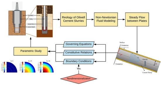
where is a constant. For , the ideas of Garboczi and Benz [61] who studied the dependence of cement diffusivity on pore structure are used. During the hydration process, the capillary pore space is gradually filled by water. The main product of the cement hydration is calcium silicate hydrate (C-S-H). Figure 1 shows the schematic of the capillary pores . The hydration products have larger volumes than the cement reactants, which explains why the cement particles in the viscous suspension develop strength from the hydration process. Two different phases contribute to the diffusivity, namely, the capillary pore space and the C-S-H gel phase. After the capillary pores close off, the smaller C-S-H gel micropores start to dominate the transport. Capillary pore space is filled with water, thus, the volume fraction of the cement particles is . The minimum capillary porosity is about 18% (known as the percolation threshold); therefore, the maximum volume fraction of cement particles is .
By considering the effects of both the capillary porosity and the C-S-H contribution on cement diffusivity, the authors proposed a relation between diffusivity and capillary pore space. After adjusting the volume fraction of cement particles with the capillary porosity , their equation becomes:
where is the diffusivity parameter;,, and are fitting coefficients with suggested values 0.001, 0.07, and 1.8; and is the Heaviside function for , for .
If we consider a steady-state condition and substitute Equation (15) into (4) with , we have [59]:
At solid boundaries, no particles can penetrate the walls, which indicates that the particle flux should be zero at the walls [63]
By integrating Equation (20), considering the boundary condition (21), we notice that for this flow field, the total flux equals zero everywhere in the flow, that is:
In summary, the following equation is used for the diffusive flux
Equations (14) and (23) form the basic constitutive relations used in this paper.
4. Flow between Two Plates
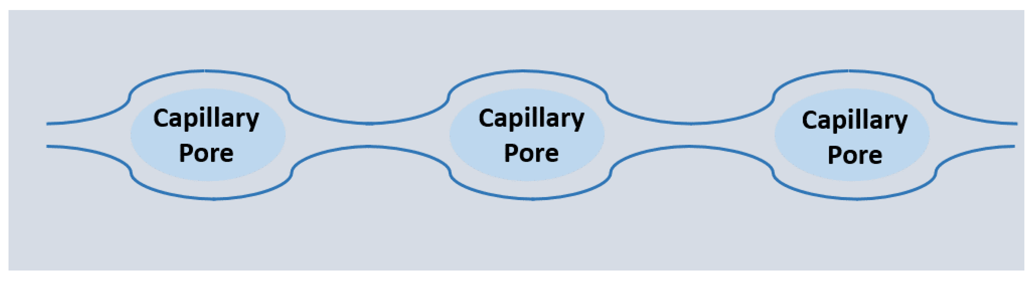
To test the models proposed in the previous section, we will solve a simple problem with relevant industrial application. As most drilling operations are done either in a vertical or a horizontal arrangement (shown in Figure 2a), we consider a tilted channel, as shown in Figure 2b where is measured from the horizontal direction. The motion is assumed to be steady and fully developed.
The velocity and the volume fraction fields are assumed to be of the form:
Using Equation (24), the conservation of mass (Equation (1)) is automatically satisfied. By substituting Equation (8) into Equation (2), the equations of linear momentum in component form become:
Let us define a modified pressure (see [64])
Then, the Equations (25) are simplified to
Equations in (27) provide the basic equations for the solution of volume fraction, velocity field, and pressure distribution in the x, y, and z-directions. In this paper, Equation (27a) is used to solve for the velocity, which is coupled to the volume fraction equation. We specify the pressure gradient in the x-direction. In a sense, we do not use Equation (27b) to solve for pressure, which will be affected by the normal stress coefficients. In more complicated flow situations and geometries, all three components of the momentum equation, along with the convection–diffusion equation, should be solved simultaneously. To obtain the expanded form of the convection–diffusion equation, we substitute Equations (12) and (15) into (22):
Before solving Equations (27a) and (28), we nondimensionalize the equations by introducing the dimensionless length and velocity as:
where H is the distance between the two plates and V is a reference velocity. The dimensionless forms for Equations (27a) and (28) become
where the following dimensionless numbers are obtained:
The physical meanings of these dimensionless numbers are: is related to the coefficient of the shear rate, related to the magnitude of shear-thinning/shear-thickening effect, is a measure of the importance of the force due to the pressure gradient and the viscous effects, is related to the gravity, and ,, are parameters related to the coefficients in the diffusion equation related to the volume concentration . In addition to these six dimensionless numbers, we also have parameters such as , which can be varied independently (see Table 1). Equations (30) and (31) are to be solved numerically, subject to appropriate physical boundary conditions. We will perform a limited parametric study to look at the effects of these dimensionless parameters on the flow and concentration profiles.
We also notice that we need two boundary conditions for and one condition for . A no-slip boundary condition for velocity at the two plates is assumed. These are:
For the volume fraction, we specify an average quantity given in terms of an integral taken across the cross section of the flow (see [65]) namely:
Note that whenever a second grade fluid or any higher grade fluid models is used, the order of the differential equations (the linear momentum equation) is raised, and additional boundary conditions are needed [66,67]; although in this problem, we are not concerned with this issue since we are not solving Equation (27b).
5. Numerical Results and Discussion
The dimensionless nonlinear ordinary differential Equations (30) and (31) with the boundary conditions (33) and (34) are solved using the MATLAB solver bvp4c for boundary value problem. The step size is set as default value in the solver. The tolerance for the maximum residue is set as 0.001. The shooting method is applied to implement in the integral form. Table 1 shows the designated values of dimensionless numbers and parameters used in this case study.
In this section, we do a basic parametric study by varying these dimensionless numbers and paramters to seetheir effects on the velocity and the concentration profiles.
5.1. Effect of
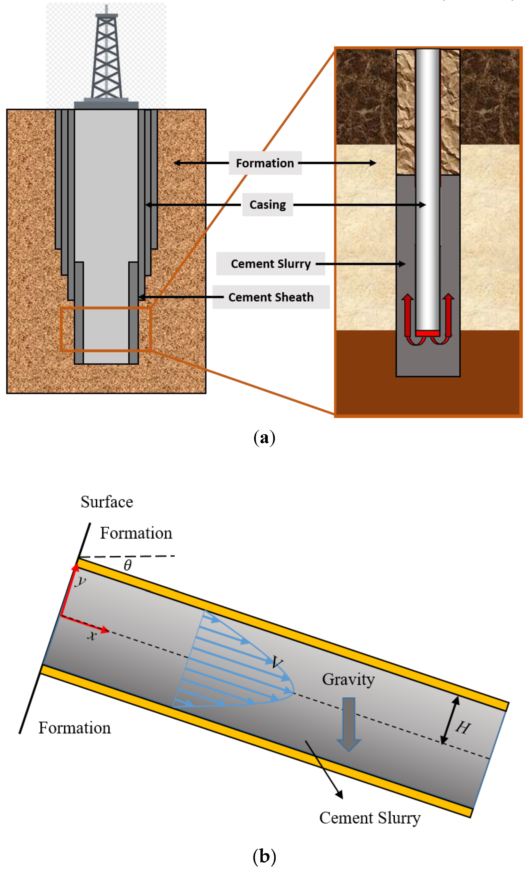
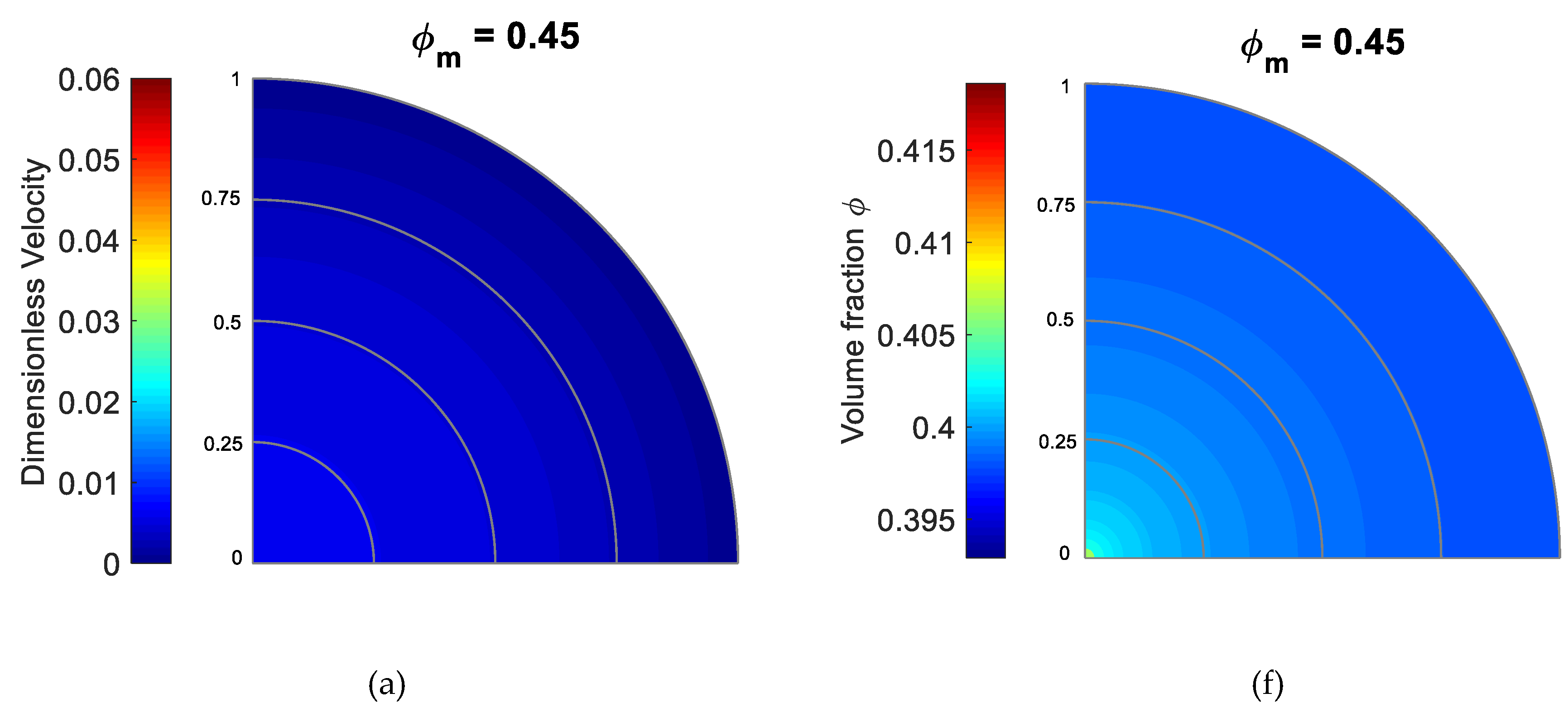
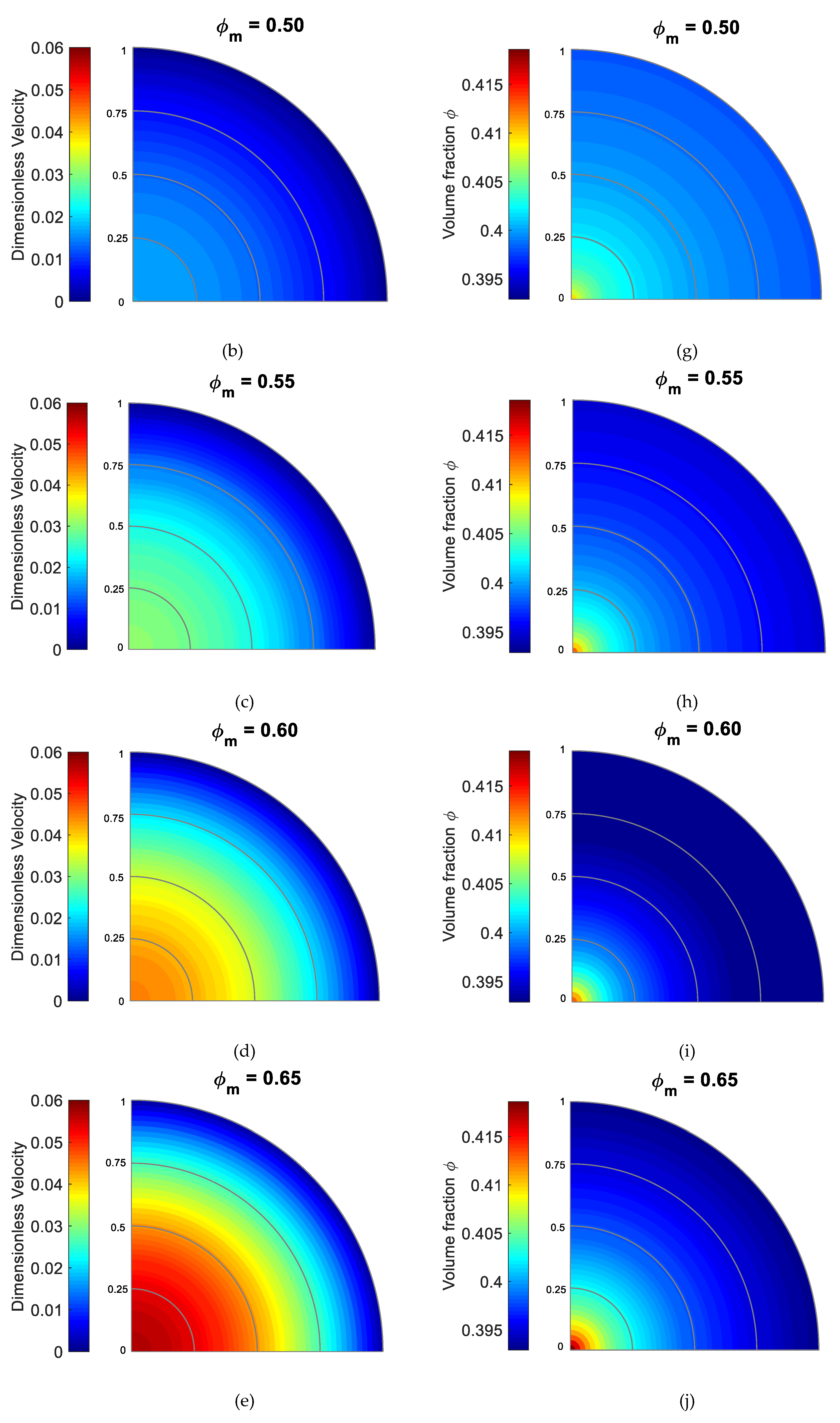
Recall that is the maximum volume fraction of the cement particles, which is usually about 0.5–0.6 [40]. Figure 3 shows the effect of on the velocity distribution and the volume fraction. Five values between 0.45 and 0.65 are selected for the parametric study. The velocity shows a parabolic distribution, and the particles tend to concentrate at the center mainly due to the effects of the first term in the particle flux Equation (15). As increases, the velocity tends to increase, and more particles tend to concentrate at the center. From Figure 4, we can see that both the velocity and the volume fraction distributions become more nonuniform for larger values of , indicating a higher packing. In a qualitative way, Phillips et al. and Wu et al. obtained similar results for the velocity profiles (see Figure 10 in [68]) and the concentration profiles (see Figure 6 in [68]).
5.2. Effect of
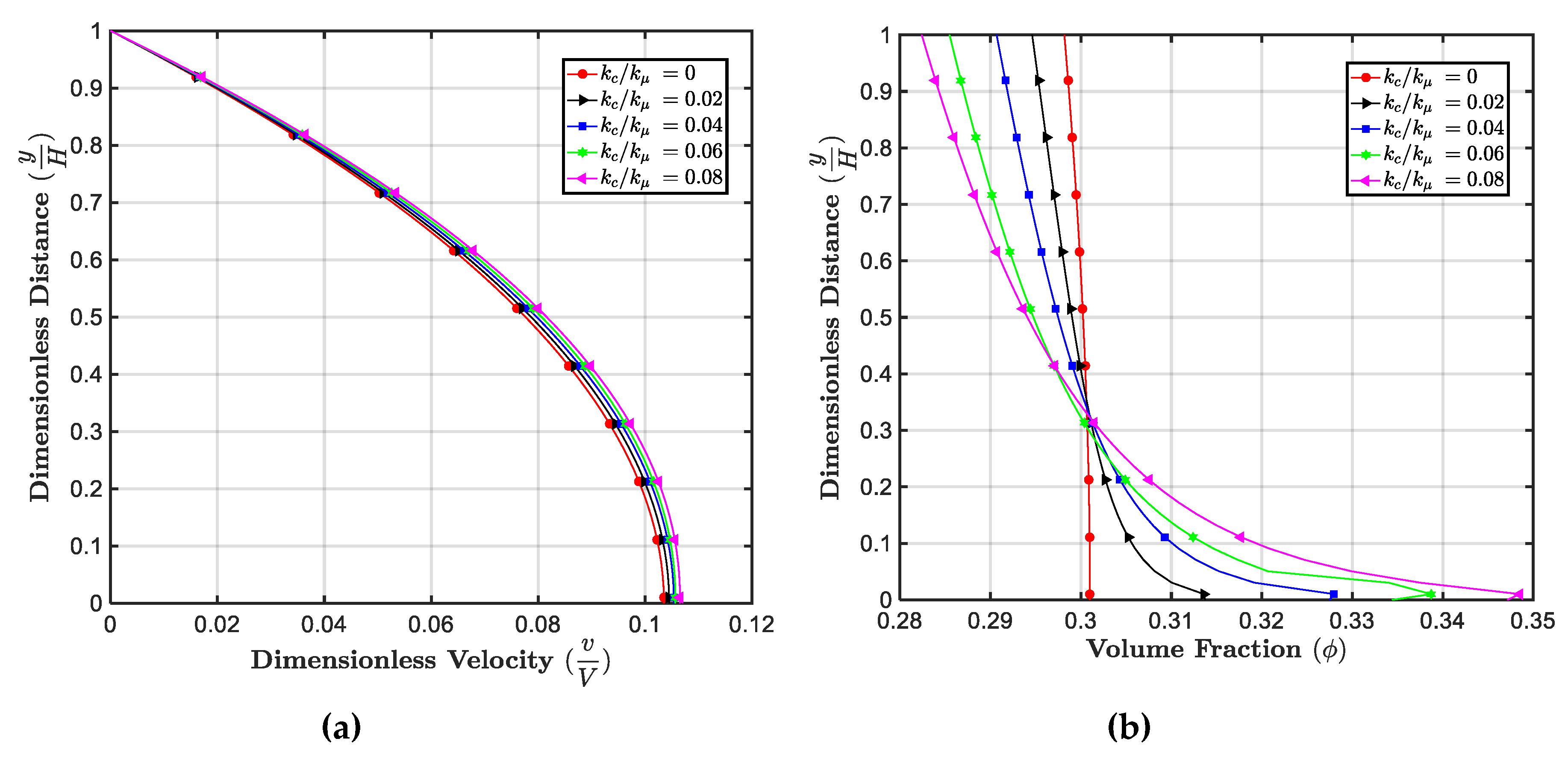
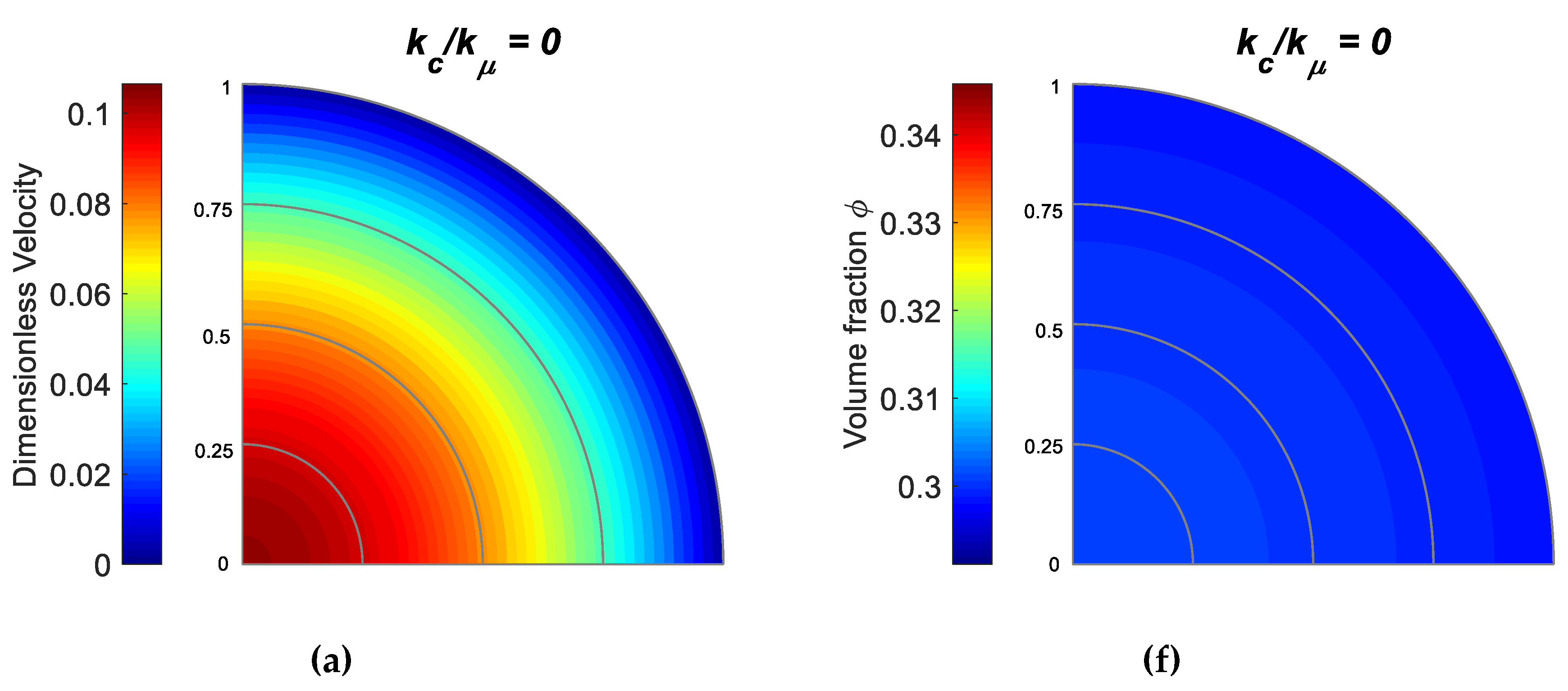
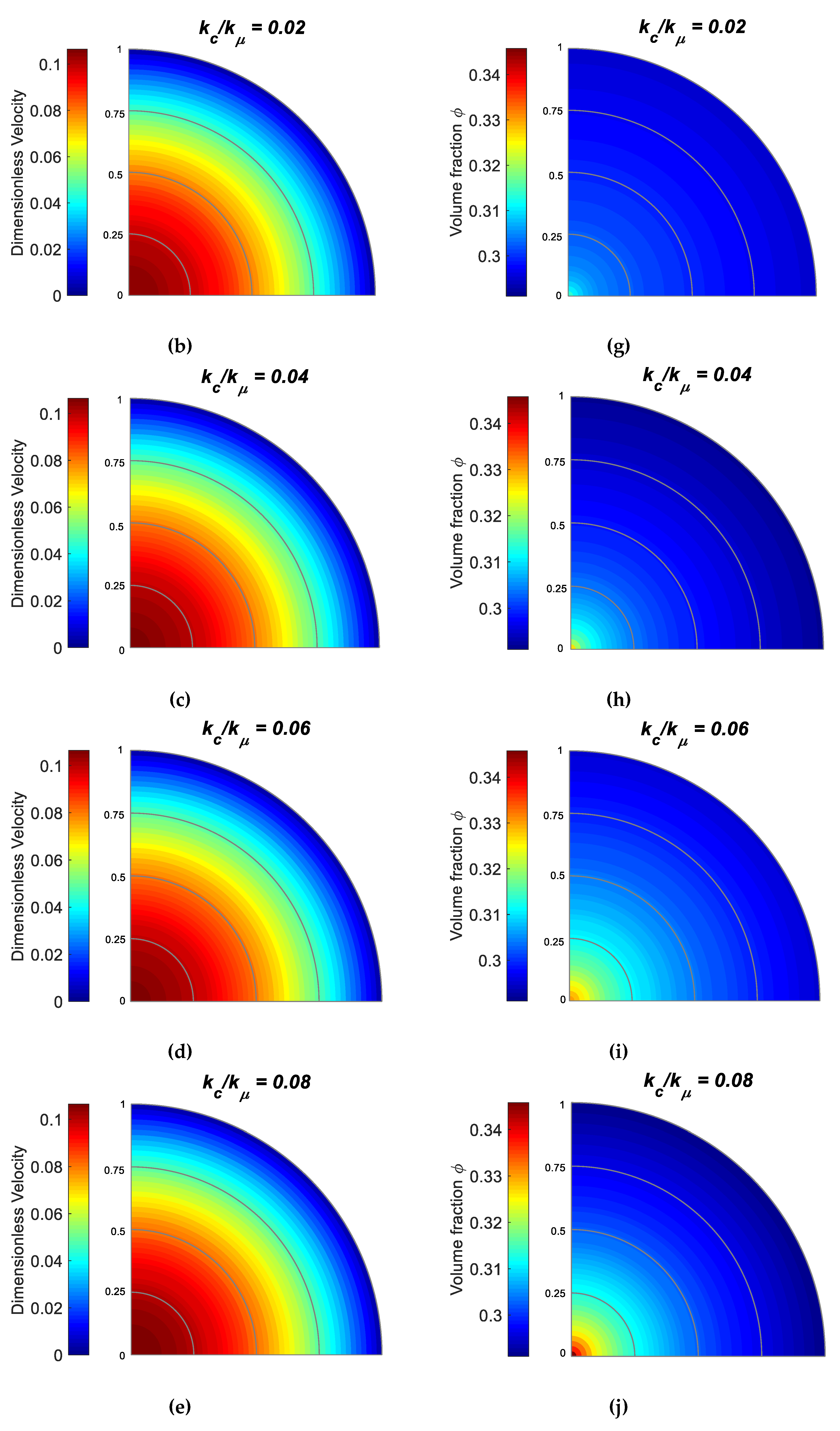
Figure 5 shows the effect of . This ratio is an indication of the effect of particles collision to the spatial variation of the viscosity. As increases, the velocity at the centerline increases a bit and the volume fraction distribution becomes more nonuniform, as shown in Figure 6. When is zero, the distribution of the volume fraction is nearly uniform. Larger values of indicate that the particles migrate towards the centerline. In a qualitative way, Wu et al. [68] obtained similar results for the effect of (see Figures 17 and 18 in [68]).
5.3. Effect of
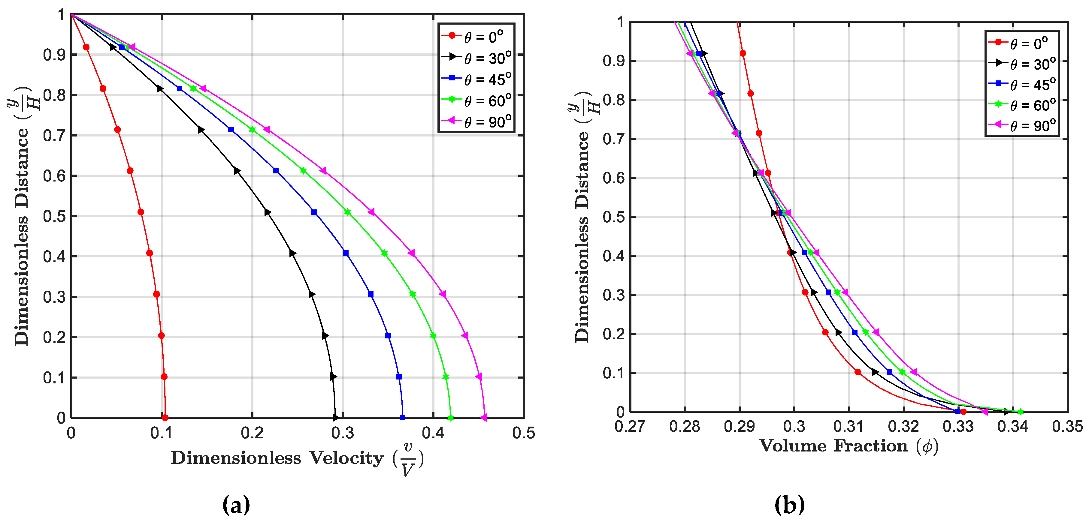
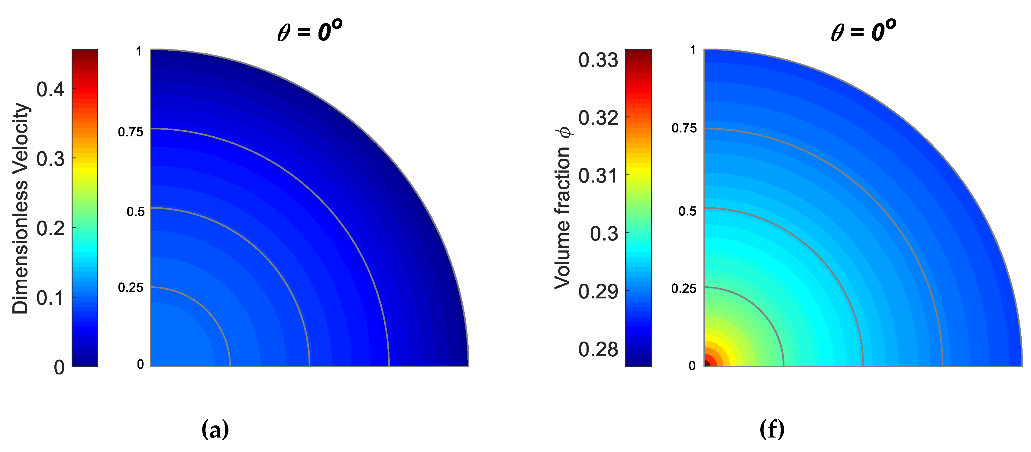
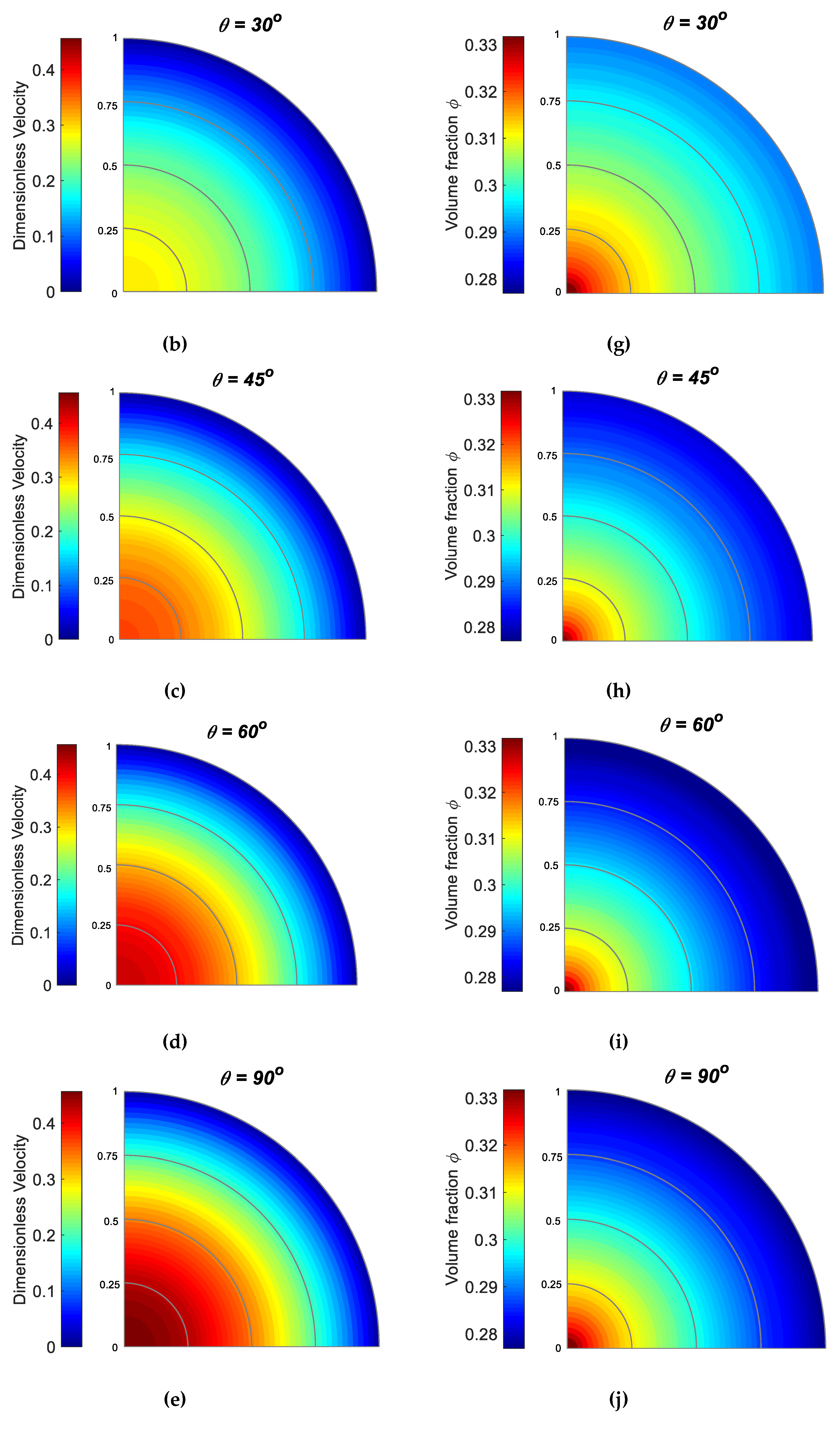
Figure 7 shows the effect of the inclination angle . For horizontal flow, = 0°, and when the two plates are in vertical arrangment = 90°. As increases, the value of the gravitational force in the x-direction increases. Larger values for result in faster flows and nonuniform velocity and volume fraction distributions, as shown in Figure 8. In other words, when the plates are inclined at a sharper angle from the horizontal direction, the particles tend to move faster and have lower concentration at the plates.
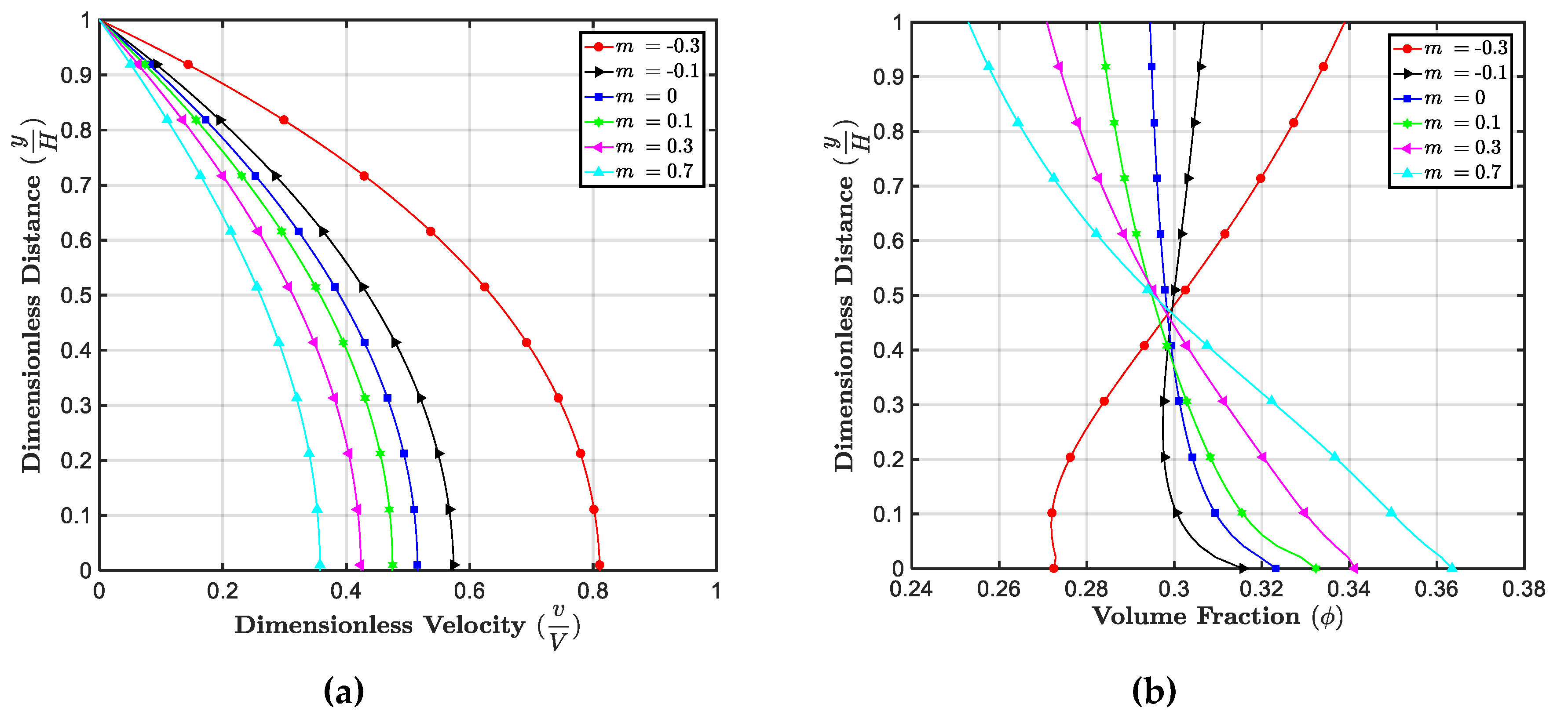
5.4. Effect of m
When m = 0, the slurry behaves as Newtonian fluid (when the viscosity does not depend on the volume fraction); when m < 0, the slurry is shear-thinning; and when m > 0, the slurry is shear-thickening. Cement slurry shows shear-thinning behavior if there are no dispersing agents while it exhibits shear-thickening behavior with the addition of dispersing acrylic polyelectrolyte [69]. Thus, we select both positive and negative values of m to study the rheological behavior of cement slurry. Figure 9 shows the effect of m on the velocity and volume fraction profiles. From the above figure, we can see that if the fluid changes from a shear-thinning fluid to a shear-thickening one (m changing from negative to positive), the velocity at the centerline decreases and the distribution of velocity becomes more linear. Similar trends could be found in Figure 2 in [68]. Larger values of m indicate more nonuniform distribution of the particles. In a qualitative way, a similar trend is observed by other researchers (see Figure 3 in [68] and Figure 2a,b in [70]).
5.5. Effect of
5.6. Effect of
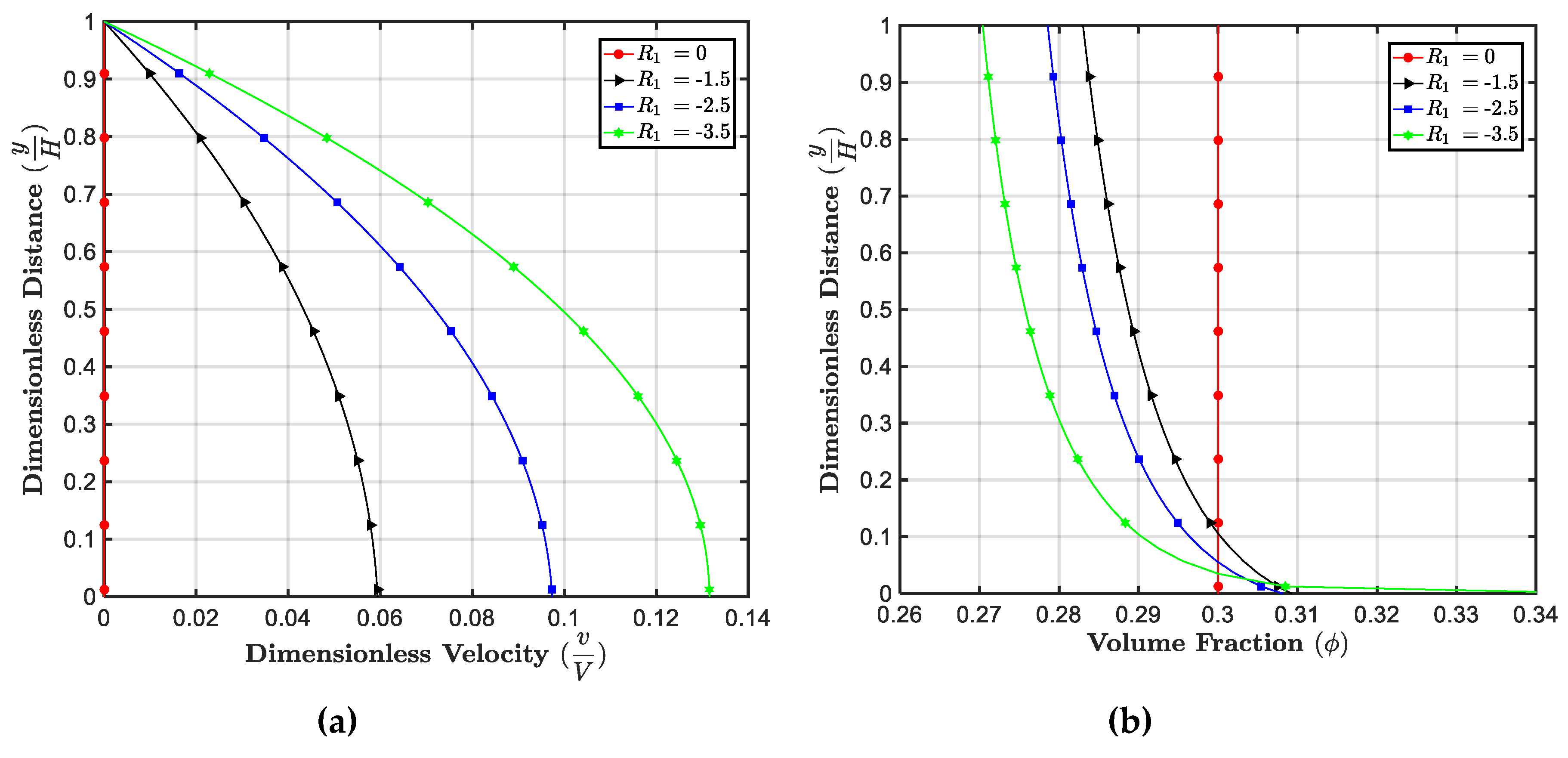
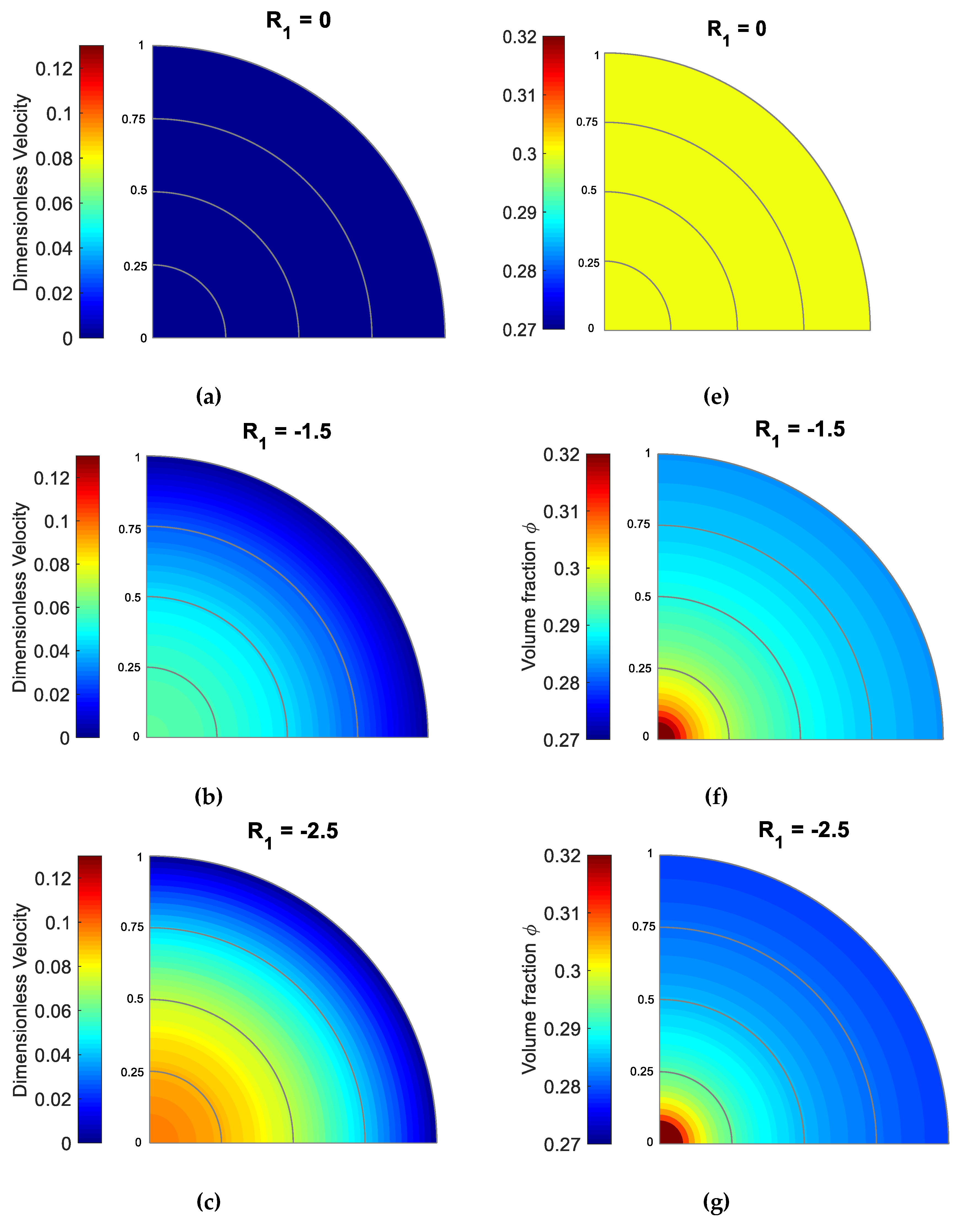
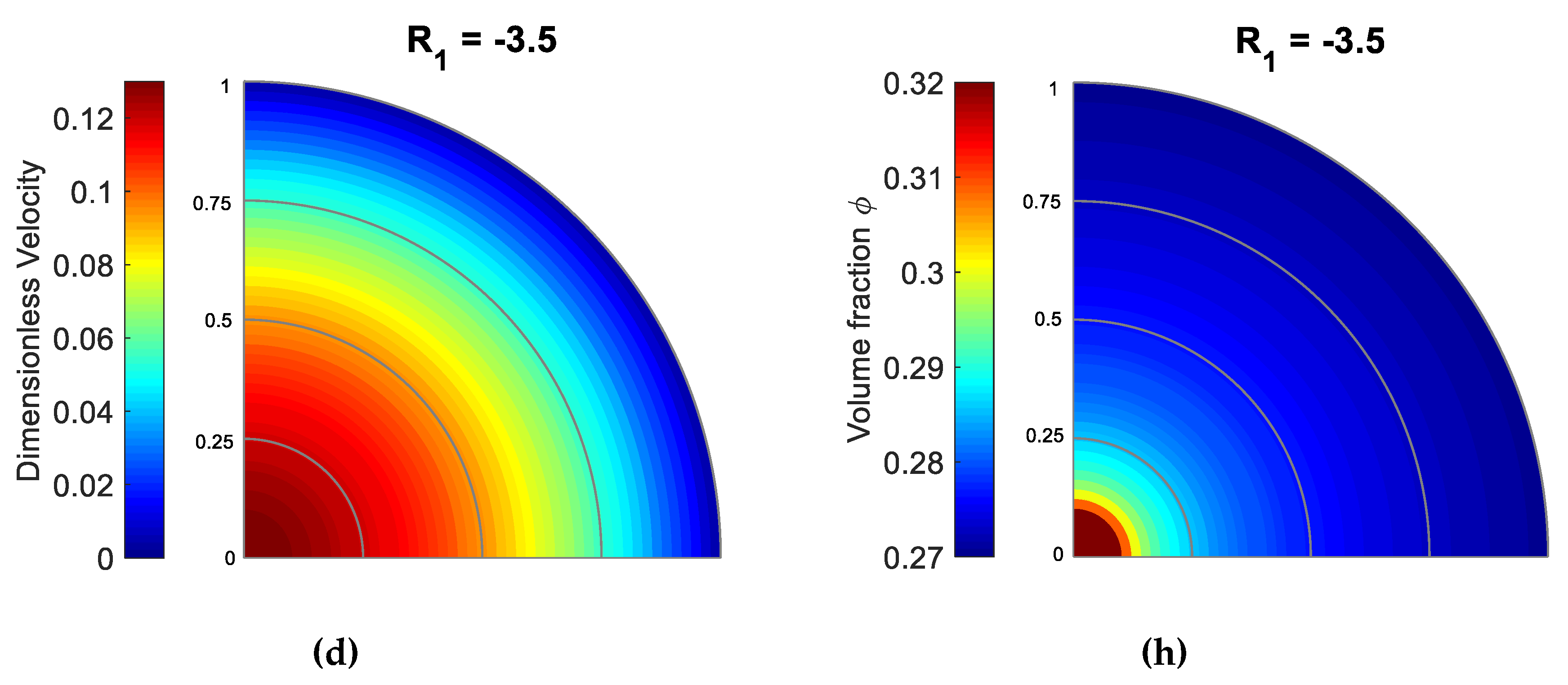
Recall that is related to the effect of pressure gradient in the x-direction. Figure 12 shows that when becomes more negative, the flow becomes faster and more particles are concentrated at the center. When , indicating no pressure gradient, a constant volume fraction profile is noticed. For larger (absolute) values of more nonuniform velocity as well as nonuniform volume fraction profiles are noticed, shown in Figure 13. Larger values for the pressure gradient indicate smaller values for the volume fraction at the plate and larger values for the volume fraction at the center. Similar trends for the effect of pressure gradient can also be found in [70] (Figure 4a,b) and [71] (Figure 2 and Figure 3).
5.7. Effect of
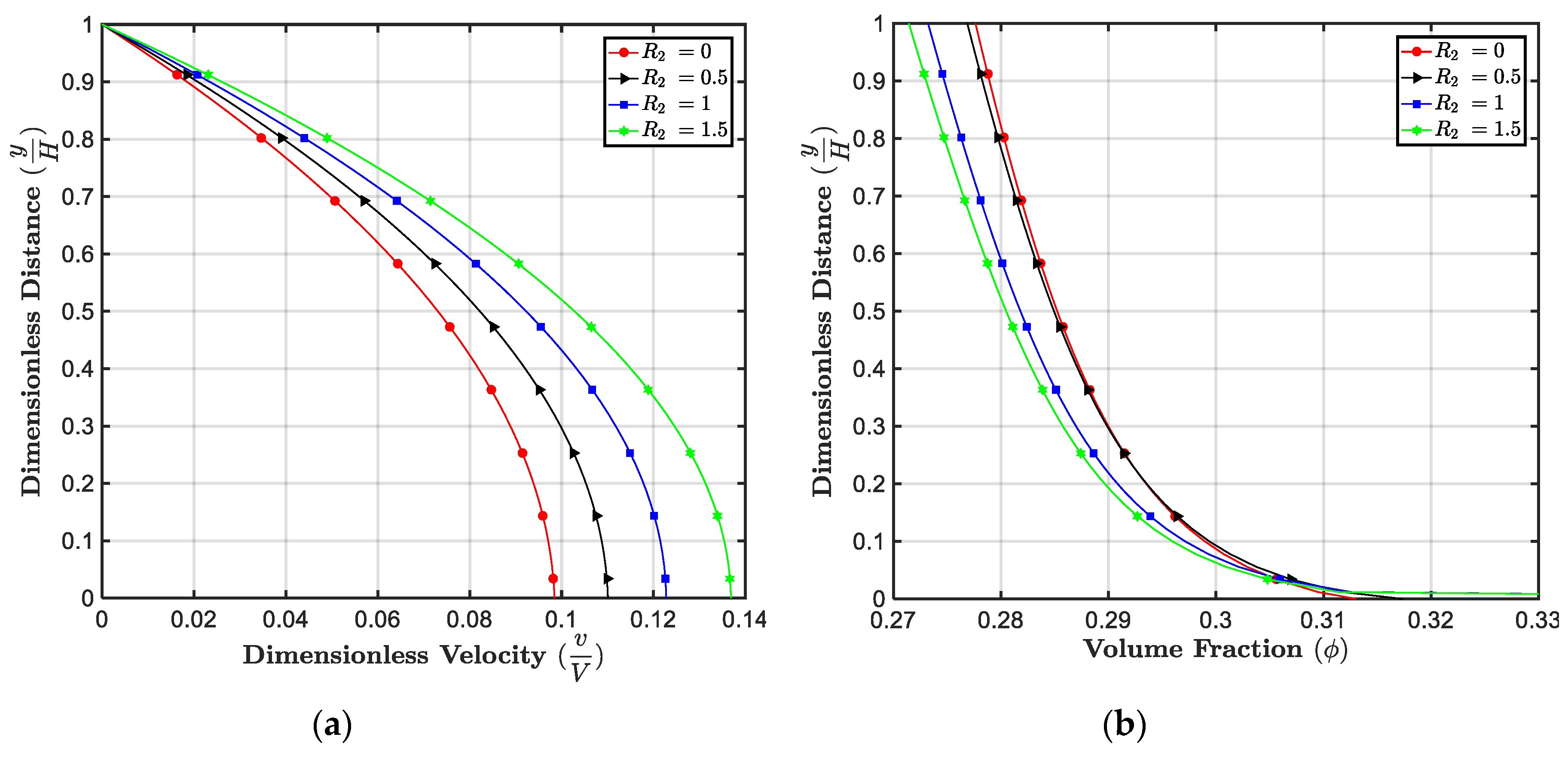
Recall that is related to the effect of the gravity term (related to the weight of the particles). As shown in Figure 14, with an increase in , the slurry has a higher centerline velocity and more particles tend to concentrate at the centerline. Both distributions of the velocity and the volume fraction become more non-uniform when increases. In a qualitative way, Miao and Massoudi [70] show similar trends for the effect of (see Figure 6a,b in their paper).
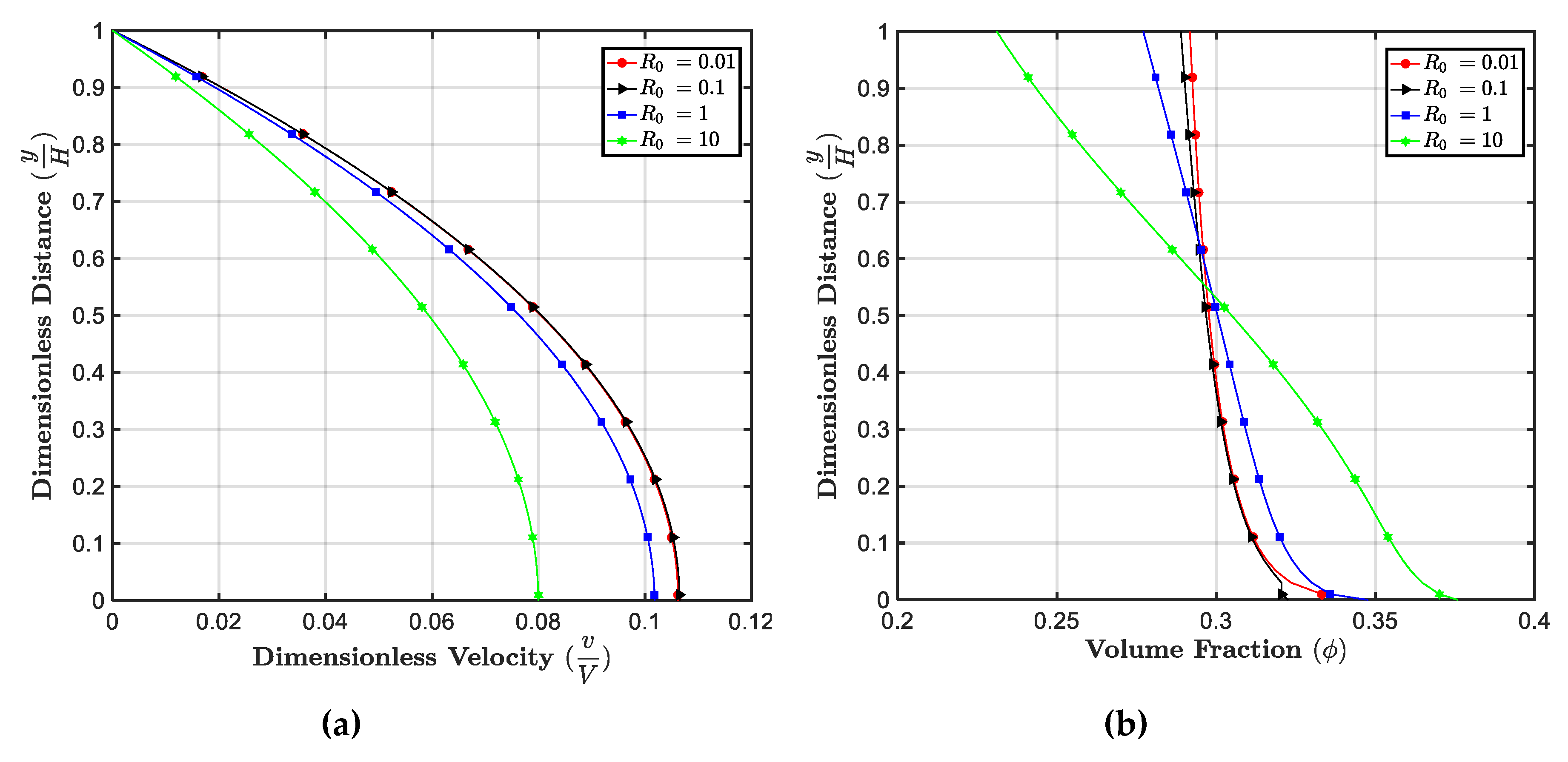
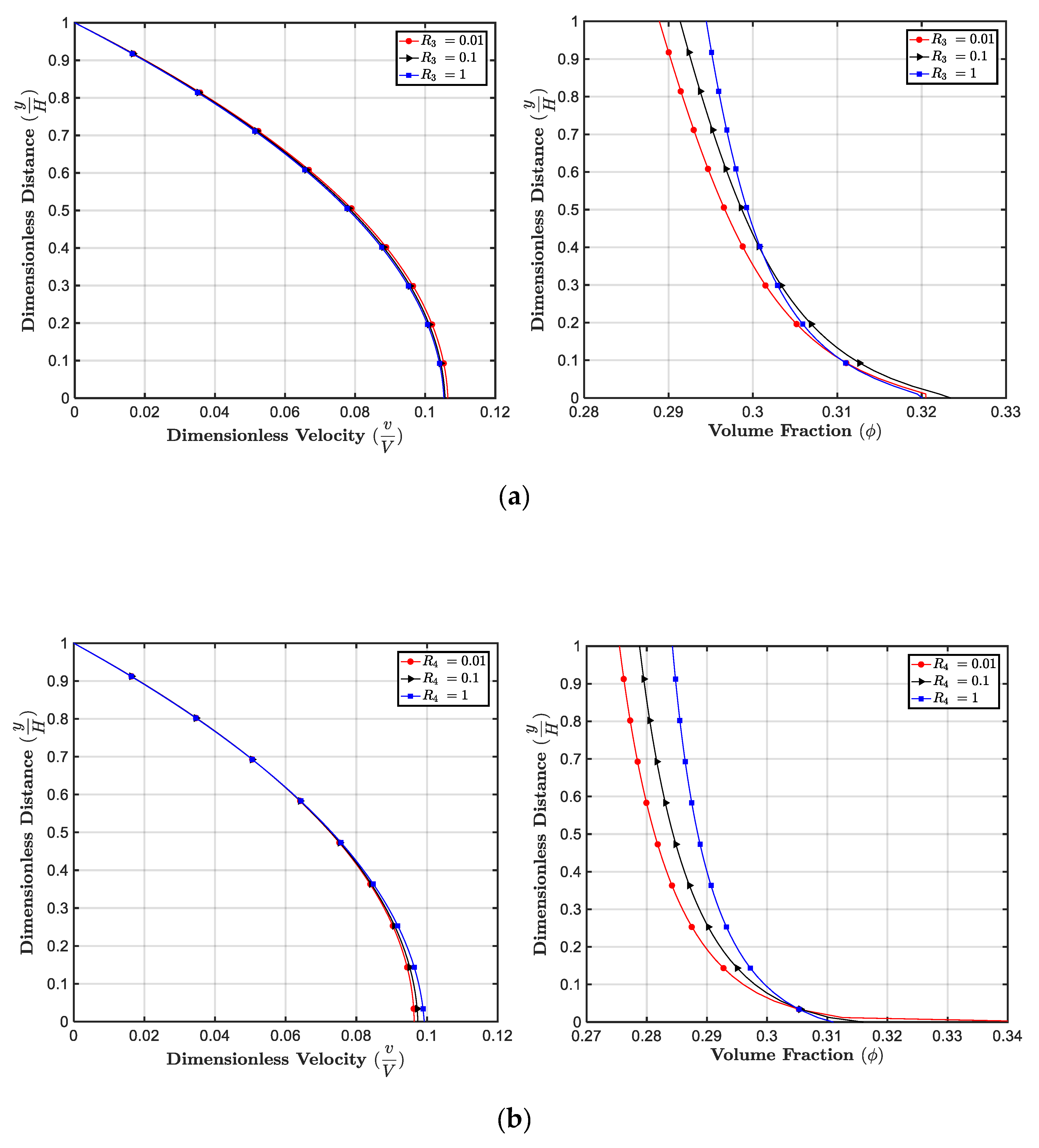
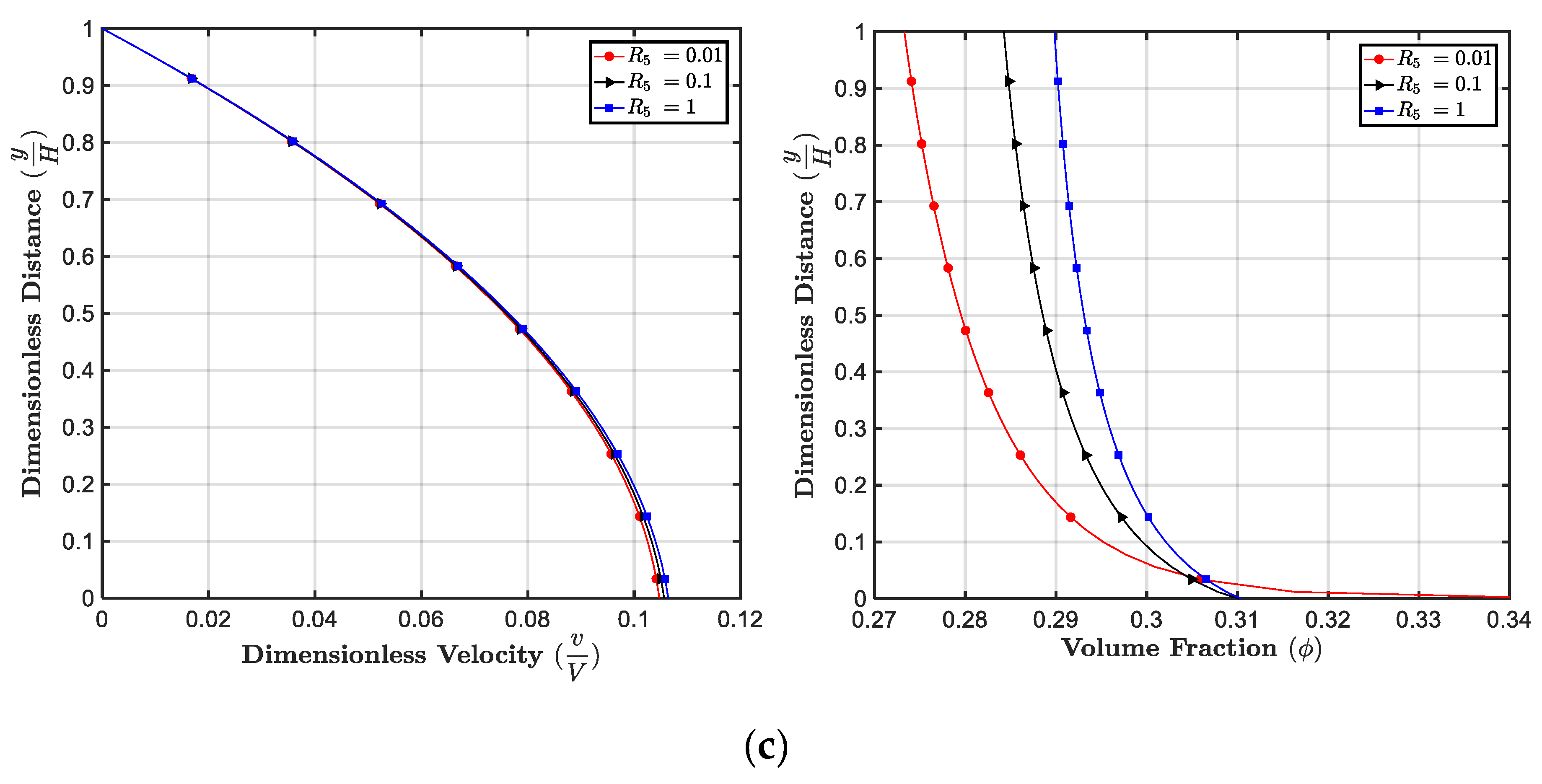
5.8. Effects of , , and
The three dimensionless numbers, , , and reflect the dependence of cement diffusivity on the volume fraction directly, as can be seen from Equation (31). They also influence the velocity profiles indirectly, as seen from Equation (30). We selected three values 0.01, 0.1, and 1 for , , and , respectively. From Figure 15, we can see that , , and have similar effects on the velocity and the volume fraction profiles. As the values of these parameters are increased, the velocity at the centerline does not change much and fewer particles tend to concentrate at the center. The volume fraction distribution becomes more uniform for larger values of , , and .
Finally, we should mention that due to the kinematical assumptions made (see Equation (24)), many of the coupling effects and the nonlinear effects in the momentum equations have disappeared. In three dimensional unsteady flows, we anticipate more interesting results due to these effects, such as the contributions from the normal stress effects, or additional flux terms, etc.
6. Conclusions
The space between the well casing and the geological formation surrounding the wellbore must be filled with cement slurry before the cement hardens. Poor understanding of rheological properties will cause the failure of the zonal isolation and can cause problems related to gas and fluid migration. Disasters, financial loss, and other serious consequences may occur from unsuccessful cementing design. Rheological behavior of cement slurry is important in the petroleum industry. In this paper, we have modeled the cement slurry as a non-Newtonian fluid (a generalized second grade fluid), where the viscosity depends on the shear rate and the particle concentration. To consider the particle transport, we use a concentration flux equation, where the coefficients of diffusivity and other fluxes depend on the shear rate and viscosity. The governing equations and the boundary conditions for flow between two plates are nondimensionalized and solved numerically. We performed a parametric study for different dimensionless numbers and the results indicate that the velocity and the volume fraction profiles are affected by the shear rate dependent viscosity and the parameters in the concentration flux equation. We also notice that the maximum packing , concentration flux parameters , the angle of inclination , pressure and gravity terms affect the velocity and particle distributions significantly. For example, we can see that the velocity and the volume fraction distributions become more nonuniform for larger values of , which indicates a higher packing. In a qualitative way, Phillips et al. and Wu et al. obtained similar results for the velocity profiles (see Figure 10 in [68]) and concentration profiles (see Figure 6 in [68]). We also notice that larger values for the pressure gradient indicate smaller values for the volume fraction at the plate but bigger values for the volume fraction at the center. Similar trends for the effect of pressure gradient can also be found in [70] (Figure 4a,b) and [71] (Figure 2 and Figure 3). For future studies, we will look at unsteady flows. Two-dimensional and three-dimensional geometries of the oil well annulus will also be studied with more advanced numerical software. More effects such as yield stress, heat transfer, and cement hydration parameters will also be considered. We should mention that in general, cement is a multi-component material, and methods of multiphase flows and mixture theories, which are more complicated can also be used to study cement slurry (for details see for example the recent papers by [72,73]).
Author Contributions
M.M. developed the framework of the paper and C.T. did most of the derivations (with help from MM) and all of the numerical simulations with some help from WTW. All authors contributed to the writing of the paper.
Funding
This research was supported by the U. S. Department of Energy, National Energy Technology Laboratory.
Acknowledgments
This paper is supported by an appointment to the U.S. Department of Energy Postgraduate Research Program for C.T. at the National Energy Technology Laboratory, administrated by the Oak Ridge Institute for Science and Education.
Disclaimer
This report was prepared as an account of work sponsored by an agency of the United States Government. Neither the United States Government nor any agency thereof, nor any of their employees, makes any warranty, express or implied, or assumes any legal liability or responsibility for the accuracy, completeness, or usefulness of any information, apparatus, product, or process disclosed, or represents that its use would not infringe privately owned rights. Reference herein to any specific commercial product, process, or service by trade name, trademark, manufacturer, or otherwise does not necessarily constitute or imply its endorsement, recommendation, or favoring by the United States Government or any agency thereof. The views and opinions of authors expressed herein do not necessarily state or reflect those of the United States Government or any agency thereof.
Conflicts of Interest
The authors declare no conflict of interest.
Nomenclature
| Symbol | Explanation |
| Density | |
| Acceleration due to gravity | |
| Characteristic length | |
| Reference velocity | |
| Particle radius | |
| Inclination angle | |
| Time | |
| Diffusion coefficient | |
| Cement diffusivity parameter | |
| Shear-rate-dependent diffusion coefficient | |
| Volume fraction-dependent diffusion coefficient | |
| Constant in volume fraction-dependent diffusion coefficient | |
| Cement diffusivity fitting coefficients | |
| Heaviside function | |
| , | Empirical coefficients for transport flux |
| Local shear rate | |
| Volume fraction of particles | |
| Capillary pore in cement | |
| Viscosity | |
| Coefficient of viscosity | |
| Effective viscosity | |
| Concentration-dependent viscosity | |
| Experimental (fitting) parameter for viscosity | |
| Maximum solid concentration | |
| Average value for the volume fraction | |
| Pressure | |
| Modified pressure | |
| Normal stress coefficients | |
| , | Material parameters |
| Dimensionless numbers | |
| Velocity vector | |
| Body force vector | |
| Particle transport flux | |
| Flux contribution due to particles collision | |
| Flux contribution due to variation in viscosity | |
| Brownian diffusive flux | |
| Cauchy stress tensor | |
| Yield stress tensor | |
| Viscous stress tensor | |
| Identity tensor | |
| Gradient of the velocity vector | |
| n-th order Rivlin–Ericksen tensor | |
| Gradient symbol | |
| Divergence operator |
References
- Mindess, S.; Young, J.F. Concrete; Prentice Hall: Englewood, NJ, USA, 1981. [Google Scholar]
- Taylor, H.F. Cement Chemistry; Thomas Telford: London, UK, 1997. [Google Scholar]
- Hanehara, S.; Yamada, K. Interaction between cement and chemical admixture from the point of cement hydration, absorption behaviour of admixture, and paste rheology. Cem. Concr. Res. 1999, 29, 1159–1165. [Google Scholar] [CrossRef]
- Vlachou, P.-V.; Piau, J.-M. Physicochemical study of the hydration process of an oil well cement slurry before setting. Cem. Concr. Res. 1999, 29, 27–36. [Google Scholar] [CrossRef]
- Barbic, L.; Tinta, V.; Lozar, B.; Marinkovic, V. Effect of Storage Time on the Rheological Behavior of Oil Well Cement Slurries. J. Am. Ceram. Soc. 1991, 74, 945–949. [Google Scholar] [CrossRef]
- Worrell, E.; Kermeli, K.; Galitsky, C. Energy Efficiency Improvement and Cost Saving Opportunities for Cement Making an ENERGY STAR® Guide for Energy and Plant Managers; EPA: Washington, DC, USA, 2013.
- Chatziaras, N.; Psomopoulos, C.S.; Themelis, N.J. Use of waste derived fuels in cement industry: A review. Manag. Environ. Qual. Int. J. 2016, 27, 178–193. [Google Scholar] [CrossRef]
- Benhelal, E.; Zahedi, G.; Shamsaei, E.; Bahadori, A. Global strategies and potentials to curb CO2 emissions in cement industry. J. Clean. Prod. 2013, 51, 142–161. [Google Scholar] [CrossRef]
- Bentz, D.P. Three-Dimensional Computer Simulation of Portland Cement Hydration and Microstructure Development. J. Am. Ceram. Soc. 1997, 80, 3–21. [Google Scholar] [CrossRef]
- Haecker, C.; Bentz, D.; Feng, X.; Stutzman, P. Prediction of cement physical properties by virtual testing. Cem. Int. 2003, 1, 86–92. [Google Scholar]
- Bullard, J.W.; Ferraris, C.; Garboczi, E.J.; Martys, N.; Stutzman, P. Virtual cement. Chapt 2004, 10, 1311–1331. [Google Scholar]
- Thomas, J.J.; Biernacki, J.J.; Bullard, J.W.; Bishnoi, S.; Dolado, J.S.; Scherer, G.W.; Luttge, A. Modeling and simulation of cement hydration kinetics and microstructure development. Cem. Concr. Res. 2011, 41, 1257–1278. [Google Scholar] [CrossRef]
- Watts, B.; Tao, C.; Ferraro, C.; Masters, F. Proficiency analysis of VCCTL results for heat of hydration and mortar cube strength. Constr. Build. Mater. 2018, 161, 606–617. [Google Scholar] [CrossRef]
- Tao, C.; Watts, B.; Ferraro, C.C.; Masters, F.J. A Multivariate Computational Framework to Characterize and Rate Virtual Portland Cements. Comput.-Aided Civ. Infrastruct. Eng. 2019, 34, 266–278. [Google Scholar] [CrossRef]
- Banfill, P.F.G.; Kitching, D.R. 14 Use of a Controlled Stress Rheometer to Study the Yield Stress of Oilwell Cement Slurries. In Rheology of Fresh Cement and Concrete: Proceedings of an International Conference, Liverpool, 1990; CRC Press: Boca Raton, FL, USA, 1990; p. 125. [Google Scholar]
- Bonett, A.; Pafitis, D. Getting to the root of gas migration. Oilfield Rev. 1996, 8, 36–49. [Google Scholar]
- Guan, S.; Rice, J.A.; Li, C.; Li, Y.; Wang, G. Structural displacement measurements using DC coupled radar with active transponder. Struct. Control Health Monit. 2017, 24, e1909. [Google Scholar] [CrossRef]
- Prohaska, M.; Ogbe, D.O.; Economides, M.J. Determining wellbore pressures in cement slurry columns. In Proceedings of the SPE Western Regional Meeting, Anchorage, AK, USA, 26–28 May 1993. [Google Scholar]
- Chenevert, M.E.; Jin, L. Model for predicting wellbore pressures in cement columns. In Proceedings of the SPE Annual Technical Conference and Exhibition, San Antonio, TX, USA, 8–11 October 1989. [Google Scholar]
- Stiles, D.A. Successful Cementing in Areas Prone to Shallow Saltwater Flows in Deep-Water Gulf of Mexico. In Proceedings of the Offshore Technology Conference, Houston, TX, USA, 5–8 May 1997. [Google Scholar]
- Brandt, W.; Dang, A.S.; Magne, E.; Crowley, D.; Houston, K.; Rennie, A.; Hodder, M.; Stringer, R.; Juiniti, R.; Ohara, S.; et al. Deepening the search for offshore hydrocarbons. Oilfield Rev. 1998, 10, 2–21. [Google Scholar]
- Wallevik, J.E. Thixotropic investigation on cement paste: Experimental and numerical approach. J. Non-Newton. Fluid Mech. 2005, 132, 86–99. [Google Scholar] [CrossRef]
- Foroushan, H.K.; Ozbayoglu, E.M.; Miska, S.Z.; Yu, M.; Gomes, P.J. On the Instability of the Cement/Fluid Interface and Fluid Mixing (includes associated erratum). SPE Drill. Complet. 2018, 33, 63–76. [Google Scholar] [CrossRef]
- Skadsem, H.J.; Kragset, S.; Lund, B.; Ytrehus, J.D.; Taghipour, A. Annular displacement in a highly inclined irregular wellbore: Experimental and three-dimensional numerical simulations. J. Pet. Sci. Eng. 2019, 172, 998–1013. [Google Scholar] [CrossRef]
- Liu, L.; Fang, Z.; Qi, C.; Zhang, B.; Guo, L.; Song, K.I.-I.L. Numerical study on the pipe flow characteristics of the cemented paste backfill slurry considering hydration effects. Powder Technol. 2019, 343, 454–464. [Google Scholar] [CrossRef]
- Murphy, E.; Lomboy, G.; Wang, K.; Sundararajan, S.; Subramaniam, S. The rheology of slurries of athermal cohesive micro-particles immersed in fluid: A computational and experimental comparison. Chem. Eng. Sci. 2019, 193, 411–420. [Google Scholar] [CrossRef]
- Slattery, J.C. Advanced Transport Phenomena; Cambridge University Press: Cambridge, UK, 1999. [Google Scholar]
- Probstein, R.F. Physicochemical Hydrodynamics: An Introduction; John Wiley & Sons: Hoboken, NJ, USA, 2005. [Google Scholar]
- Struble, L.; Sun, G.-K. Viscosity of Portland cement paste as a function of concentration. Adv. Cem. Based Mater. 1995, 2, 62–69. [Google Scholar] [CrossRef]
- Banfill, P.F. The rheology of fresh cement and concrete-a review. In Proceedings of the 11th international cement chemistry congress, Durban, South Africa, 11–16 May 2003; Volume 1, pp. 50–62. [Google Scholar]
- Gandelman, R.; Miranda, C.; Teixeira, K.; Martins, A.L.; Waldmann, A. On the rheological parameters governing oilwell cement slurry stability. Annu. Trans. Nord. Rheol. Soc. 2004, 12, 85–91. [Google Scholar]
- Tattersall, G.H.; Banfill, P.F. The Rheology of Fresh Concrete; Pitman Advanced Publishing Program: London, UK, 1983. [Google Scholar]
- Moon, J.; Wang, S. Acoustic method for determining the static gel strength of slurries. In Proceedings of the SPE Rocky Mountain Regional Meeting, Gillette, WY, USA, 15–18 May 1999. [Google Scholar]
- Bellotto, M. Cement paste prior to setting: A rheological approach. Cem. Concr. Res. 2013, 52, 161–168. [Google Scholar] [CrossRef]
- Barnes, H.A. Thixotropy—A review. J. Non-Newton. Fluid Mech. 1997, 70, 1–33. [Google Scholar] [CrossRef]
- Mewis, J.; Wagner, N.J. Colloidal Suspension Rheology; Cambridge University Press: Cambridge, UK, 2012. [Google Scholar]
- Barnes, H.A. The yield stress—A review or ‘παντα ρει’—Everything flows? J. Non-Newton. Fluid Mech. 1999, 81, 133–178. [Google Scholar] [CrossRef]
- Carreau, P.J.; de Kee, D.C.R.; Chhabra, R.P. Rheology of Polymeric Systems: Principles and Applications; Hanser: New York, NY, USA, 1997. [Google Scholar]
- Carreau, P.J.; de Kee, D. Review of some useful rheological equations. Can. J. Chem. Eng. 1979, 57, 3–15. [Google Scholar] [CrossRef]
- Justnes, H.; Vikan, H. Viscosity of cement slurries as a function of solids content. Ann. Trans. Nord. Rheol. Soc. 2005, 13, 75–82. [Google Scholar]
- Asaga, K.; Roy, D.M. Rheological properties of cement mixes: IV. Effects of superplasticizers on viscosity and yield stress. Cem. Concr. Res. 1980, 10, 287–295. [Google Scholar] [CrossRef]
- Vand, V. Viscosity of solutions and suspensions. I. Theory. J. Phys. Chem. 1948, 52, 277–299. [Google Scholar] [CrossRef]
- Roscoe, R. The viscosity of suspensions of rigid spheres. Br. J. Appl. Phys. 1952, 3, 267. [Google Scholar] [CrossRef]
- Bonen, D.; Shah, S.P. Fresh and hardened properties of self-consolidating concrete. Prog. Struct. Eng. Mater. 2005, 7, 14–26. [Google Scholar] [CrossRef]
- Chougnet, A.; Palermo, T.; Audibert, A.; Moan, M. Rheological behaviour of cement and silica suspensions: Particle aggregation modelling. Cem. Concr. Res. 2008, 38, 1297–1301. [Google Scholar] [CrossRef]
- Tregger, N.A.; Pakula, M.E.; Shah, S.P. Influence of clays on the rheology of cement pastes. Cem. Concr. Res. 2010, 40, 384–391. [Google Scholar] [CrossRef]
- Bentz, D.P.; Ferraris, C.F.; Galler, M.A.; Hansen, A.S.; Guynn, J.M. Influence of particle size distributions on yield stress and viscosity of cement–fly ash pastes. Cem. Concr. Res. 2012, 42, 404–409. [Google Scholar] [CrossRef]
- Ouyang, J.; Tan, Y. Rheology of fresh cement asphalt emulsion pastes. Constr. Build. Mater. 2015, 80, 236–243. [Google Scholar] [CrossRef]
- O’Neill, R.; McCarthy, H.O.; Montufar, E.B.; Ginebra, M.P.; Wilson, D.I.; Lennon, A.; Dunne, N. Critical review: Injectability of calcium phosphate pastes and cements. Acta Biomater. 2017, 50, 1–19. [Google Scholar] [CrossRef] [PubMed] [Green Version]
- Massoudi, M. Constitutive modelling of flowing granular materials: A continuum approach. In Granular Materials: Fundamentals and Applications; The Royal Society of Chemistry: Cambridge, UK, 2004; Volume 63. [Google Scholar]
- Massoudi, M.; Mehrabadi, M.M. A continuum model for granular materials: Considering dilatancy and the Mohr-Coulomb criterion. Acta Mech. 2001, 152, 121–138. [Google Scholar] [CrossRef]
- Rivlin, R.S. Further remarks on the stress-deformation relations for isotropic materials. J. Ration. Mech. Anal. 1955, 4, 681–702. [Google Scholar] [CrossRef]
- Truesdell, C.; Noll, W. The Non-linear Field Theories of Mechanics; Springer: Berlin, Germany, 1992. [Google Scholar]
- Man, C.-S.; Sun, Q.-X. On the significance of normal stress effects in the flow of glaciers. J. Glaciol. 1987, 33, 268–273. [Google Scholar] [CrossRef]
- Man, C.-S. Nonsteady channel flow of ice as a modified second-order fluid with power-law viscosity. Arch. Ration. Mech. Anal. 1992, 119, 35–57. [Google Scholar] [CrossRef]
- Dunn, J.E.; Fosdick, R.L. Thermodynamics, stability, and boundedness of fluids of complexity 2 and fluids of second grade. Arch. Ration. Mech. Anal. 1974, 56, 191–252. [Google Scholar] [CrossRef]
- Massoudi, M.; Vaidya, A. On some generalizations of the second grade fluid model. Nonlinear Anal. Real World Appl. 2008, 9, 1169–1183. [Google Scholar] [CrossRef]
- Phillips, R.J.; Armstrong, R.C.; Brown, R.A.; Graham, A.L.; Abbott, J.R. A constitutive equation for concentrated suspensions that accounts for shear-induced particle migration. Phys. Fluids A Fluid Dyn. 1992, 4, 30–40. [Google Scholar] [CrossRef]
- Li, Y.; Wu, W.-T.; Liu, X.; Massoudi, M. The effects of particle concentration and various fluxes on the flow of a fluid-solid suspension. Appl. Math. Comput. 2019, 358, 151–160. [Google Scholar] [CrossRef]
- Bridges, C.; Rajagopal, K.R. Pulsatile flow of a chemically-reacting nonlinear fluid. Comput. Math. Appl. 2006, 52, 1131–1144. [Google Scholar] [CrossRef]
- Garboczi, E.J.; Bentz, D.P. Computer simulation of the diffusivity of cement-based materials. J. Mater. Sci. 1992, 27, 2083–2092. [Google Scholar] [CrossRef]
- Snyder, K.A.; Bentz, D.P. Suspended hydration and loss of freezable water in cement pastes exposed to 90% relative humidity. Cem. Concr. Res. 2004, 34, 2045–2056. [Google Scholar] [CrossRef]
- Wu, W.-T.; Aubry, N.; Antaki, J.; McKoy, M.; Massoudi, M. Heat transfer in a drilling fluid with geothermal applications. Energies 2017, 10, 1349. [Google Scholar] [CrossRef]
- Gupta, G.; Massoudi, M. Flow of a generalized second grade fluid between heated plates. Acta Mech. 1993, 99, 21–33. [Google Scholar] [CrossRef]
- Massoudi, M. Boundary conditions in mixture theory and in CFD applications of higher order models. Comput. Math. Appl. 2007, 53, 156–167. [Google Scholar] [CrossRef] [Green Version]
- Dunn, J.E.; Rajagopal, K.R. Fluids of differential type: Critical review and thermodynamic analysis. Int. J. Eng. Sci. 1995, 33, 689–729. [Google Scholar] [CrossRef] [Green Version]
- Rajagopal, K.R.; Kaloni, P.N. Some remarks on boundary conditions for flows of fluids of the differential type. Contin. Mech. Appl. 1989, 48, 935–942. [Google Scholar]
- Wu, W.-T.; Massoudi, M. Heat transfer and dissipation effects in the flow of a drilling fluid. Fluids 2016, 1, 4. [Google Scholar] [CrossRef]
- Lootens, D.; Hébraud, P.; Lécolier, E.; van Damme, H. Gelation, Shear-Thinning and Shear-Thickening in Cement Slurries. Oil Gas Sci. Technol. 2004, 59, 31–40. [Google Scholar] [CrossRef]
- Miao, L.; Massoudi, M. Heat transfer analysis and flow of a slag-type fluid: Effects of variable thermal conductivity and viscosity. Int. J. Non-Linear Mech. 2015, 76, 8–19. [Google Scholar] [CrossRef]
- Gudhe, R.; Yalamanchili, R.C.; Massoudi, M. The flow of granular materials in a pipe: Numerical solutions. ASME Appl. Mech. Div.-Publ.-AMD 1993, 160, 41. [Google Scholar]
- Massoudi, M. A note on the meaning of mixture viscosity using the classical continuum theories of mixtures. Int. J. Eng. Sci. 2008, 46, 677–689. [Google Scholar] [CrossRef]
- Massoudi, M. A Mixture Theory formulation for hydraulic or pneumatic transport of solid particles. Int. J. Eng. Sci. 2010, 48, 1440–1461. [Google Scholar] [CrossRef]
Figure 1.
Schematic of capillary pores , lined with C-S-H [62].
Figure 1.
Schematic of capillary pores , lined with C-S-H [62].

Figure 2.
Schematic diagram of (a) oil well cementing and (b) cement slurry flow in a tilted channel.
Figure 2.
Schematic diagram of (a) oil well cementing and (b) cement slurry flow in a tilted channel.

Figure 3.
Effect of on (a) the velocity; and (b) the volume fraction profiles, with 1.82, 0.4, 0.1, −2.5, 0.1, 0.01, 0.07, 1.8, 0.05, 1, 45o.
Figure 3.
Effect of on (a) the velocity; and (b) the volume fraction profiles, with 1.82, 0.4, 0.1, −2.5, 0.1, 0.01, 0.07, 1.8, 0.05, 1, 45o.

Figure 4.
Distribution of the velocity for (a) = 0.45; (b) = 0.50; (c) = 0.55; (d) = 0.60; (e) = 0.65; and the cement volume concentration for (f) = 0.45; (g) = 0.50; (h) = 0.55; (i) = 0.60; (j) = 0.65.
Figure 4.
Distribution of the velocity for (a) = 0.45; (b) = 0.50; (c) = 0.55; (d) = 0.60; (e) = 0.65; and the cement volume concentration for (f) = 0.45; (g) = 0.50; (h) = 0.55; (i) = 0.60; (j) = 0.65.


Figure 5.
Effect of on (a) the velocity; and (b) the volume fraction profiles, with 1.82, 0.3, 0.1, −2.5, 0.1, 0.01, 0.07, 1.8, 0.65, 1, 45o.
Figure 5.
Effect of on (a) the velocity; and (b) the volume fraction profiles, with 1.82, 0.3, 0.1, −2.5, 0.1, 0.01, 0.07, 1.8, 0.65, 1, 45o.

Figure 6.
Distribution of the velocity for (a) = 0; (b) = 0.02; (c) = 0.04; (d) = 0.06; (e) = 0.08; and the cement volume concentration for (f) = 0; (g) = 0.02; (h) = 0.04; (i) = 0.06; (j) = 0.08.
Figure 6.
Distribution of the velocity for (a) = 0; (b) = 0.02; (c) = 0.04; (d) = 0.06; (e) = 0.08; and the cement volume concentration for (f) = 0; (g) = 0.02; (h) = 0.04; (i) = 0.06; (j) = 0.08.


Figure 7.
Effect of on (a) the velocity; and (b) the volume fraction profiles, with 1.82, 0.3, 0.1, -2.5, 10, 0.01, 0.07, 1.8, 0.05, 0.65, 1.
Figure 7.
Effect of on (a) the velocity; and (b) the volume fraction profiles, with 1.82, 0.3, 0.1, -2.5, 10, 0.01, 0.07, 1.8, 0.05, 0.65, 1.

Figure 8.
Distribution of the velocity for (a) = 0°; (b) = 30°; (c) = 45°; (d) = 60°; (e) = 90°; and the cement volume concentration for (f) = 0°; (g) = 30°; (h) = 45°; (i) = 60°; (j) = 90°.
Figure 8.
Distribution of the velocity for (a) = 0°; (b) = 30°; (c) = 45°; (d) = 60°; (e) = 90°; and the cement volume concentration for (f) = 0°; (g) = 30°; (h) = 45°; (i) = 60°; (j) = 90°.


Figure 9.
Effect of m on (a) the velocity; and (b) the volume fraction profiles, with 1.82, 0.3, 0.1, −2.5, 10, 0.01, 0.07, 1.8, 0.05, 0.65, 90°.
Figure 9.
Effect of m on (a) the velocity; and (b) the volume fraction profiles, with 1.82, 0.3, 0.1, −2.5, 10, 0.01, 0.07, 1.8, 0.05, 0.65, 90°.

Figure 10.
Effect of on (a) the velocity; and (b) the volume fraction profiles, with 1.82, 0.3, −2.5, 0.1, 0.01, 0.07, 1.8, 0.05, 0.65, 1, 45o.
Figure 10.
Effect of on (a) the velocity; and (b) the volume fraction profiles, with 1.82, 0.3, −2.5, 0.1, 0.01, 0.07, 1.8, 0.05, 0.65, 1, 45o.

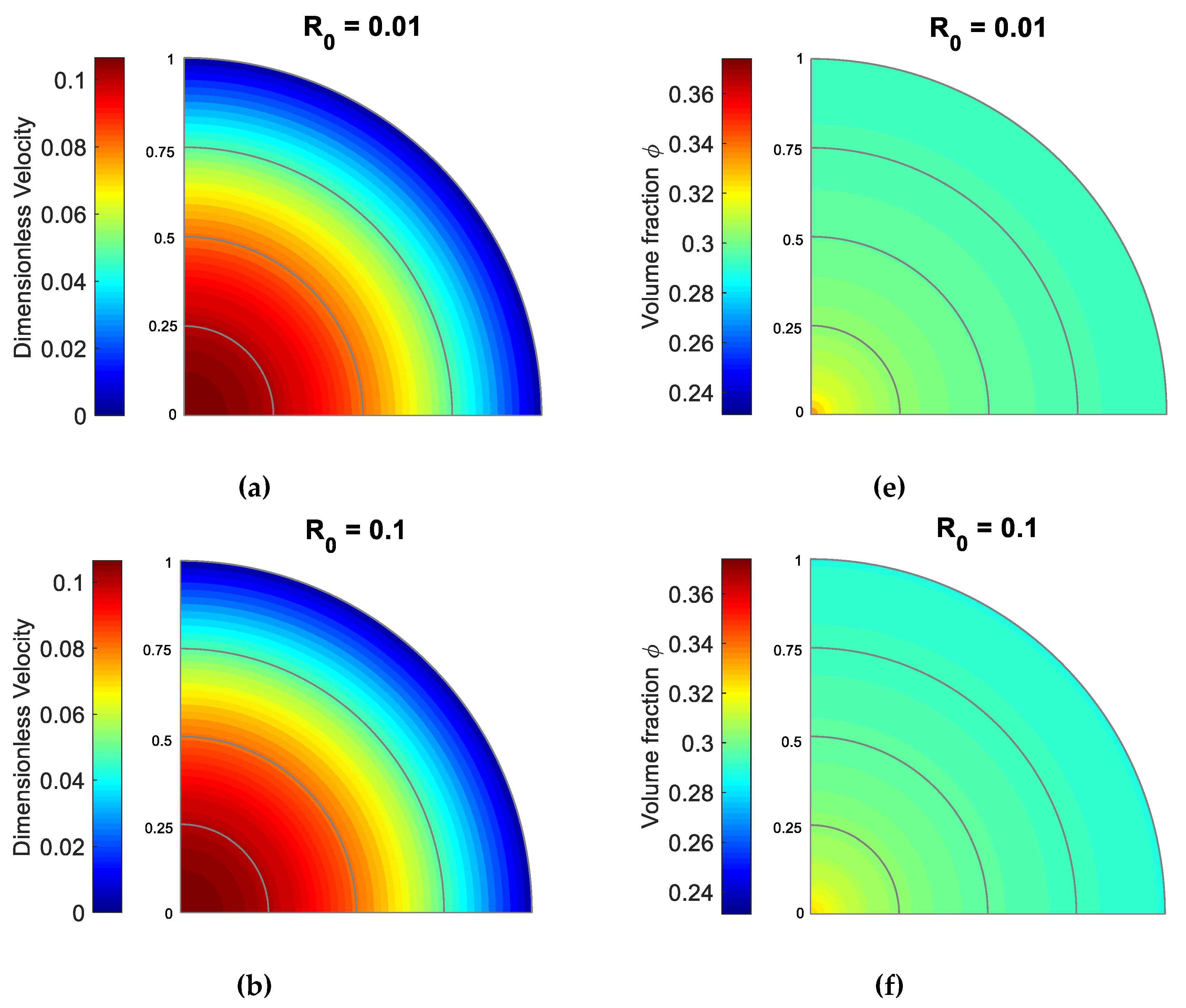
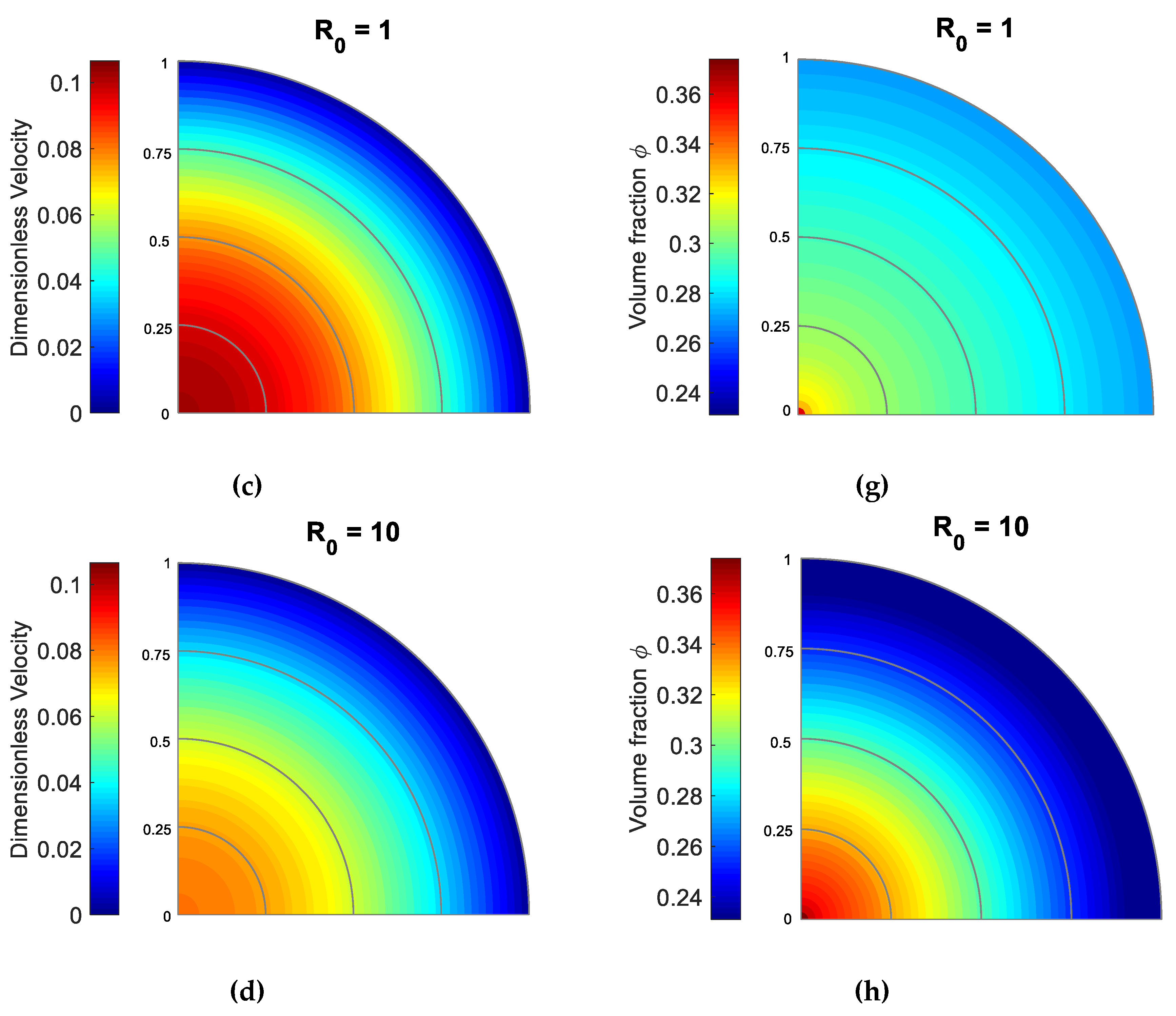
Figure 11.
Distribution of the velocity for (a) = 0.01; (b) = 0.1; (c) = 1; (d) = 10; and the cement volume concentration for (e) = 0.01; (f) = 0.1; (g) = 1; (h) = 10.
Figure 11.
Distribution of the velocity for (a) = 0.01; (b) = 0.1; (c) = 1; (d) = 10; and the cement volume concentration for (e) = 0.01; (f) = 0.1; (g) = 1; (h) = 10.


Figure 12.
Effect of on (a) the velocity; and (b) the volume fraction profiles, with 1.82, 0.3, 0.1, 0.1, 0.01, 0.07, 1.8, 0.05, 0.65, 1, 45°.
Figure 12.
Effect of on (a) the velocity; and (b) the volume fraction profiles, with 1.82, 0.3, 0.1, 0.1, 0.01, 0.07, 1.8, 0.05, 0.65, 1, 45°.

Figure 13.
Distribution of the velocity for (a) = 0; (b) = −1.5; (c) = −2.5; (d) = −3.5; and the cement volume concentration for (e) = 0; (f) = −1.5; (g) = −2.5; (h) = −3.5.
Figure 13.
Distribution of the velocity for (a) = 0; (b) = −1.5; (c) = −2.5; (d) = −3.5; and the cement volume concentration for (e) = 0; (f) = −1.5; (g) = −2.5; (h) = −3.5.


Figure 14.
Effect of on (a) the velocity; and (b) the volume fraction profiles, with 1.82, 0.3, 0.1, −2.5, 0.01, 0.07, 1.8, 0.05, 0.65, 1, 45°.
Figure 14.
Effect of on (a) the velocity; and (b) the volume fraction profiles, with 1.82, 0.3, 0.1, −2.5, 0.01, 0.07, 1.8, 0.05, 0.65, 1, 45°.

Figure 15.
(a) Effect of on the velocity and the volume fraction profiles, with 1.82, 0.3, 0.1, −2.5, 0.1, 0.07, 1.8, 0.05, 0.65, 1, 45°; (b) effect of on the velocity and volume fraction profile, with 1.82, 0.3, 0.1, −2.5, 0.1, 0.01, 1.8, 0.05, 0.65, 1, 45°; and (c) effect of on the velocity and volume fraction profile, with 1.82, 0.3, 0.1, −2.5, 0.1, 0.01, 0.07, 0.05, 0.65, 1, 45°.


Table 1.
Values of the dimensionless numbers and other parameters.
| Parameters | Range of Values |
|---|---|
| 0.45, 0.5, 0.55, 0.6, 0.65 | |
| 0, 0.02, 0.04, 0.06, 0.08 | |
| 0°, 30°, 45°, 60°, 90° | |
| −0.3, −0.1, 0, 0.1, 0.3, 0.7 | |
| 0.01, 0.1, 1, 10 | |
| 0, −1.5, −2.5, −3.5 | |
| 0, 0.5, 1, 1.5 | |
| 0.01, 0.1, 1 | |
| 0.01, 0.1, 1 | |
| 0.01, 0.1, 1 |
© 2019 by the authors. Licensee MDPI, Basel, Switzerland. This article is an open access article distributed under the terms and conditions of the Creative Commons Attribution (CC BY) license (http://creativecommons.org/licenses/by/4.0/).
Share and Cite
MDPI and ACS Style
Tao, C.; Kutchko, B.G.; Rosenbaum, E.; Wu, W.-T.; Massoudi, M. Steady Flow of a Cement Slurry. Energies 2019, 12, 2604. https://doi.org/10.3390/en12132604
AMA Style
Tao C, Kutchko BG, Rosenbaum E, Wu W-T, Massoudi M. Steady Flow of a Cement Slurry. Energies. 2019; 12(13):2604. https://doi.org/10.3390/en12132604
Chicago/Turabian StyleTao, Chengcheng, Barbara G. Kutchko, Eilis Rosenbaum, Wei-Tao Wu, and Mehrdad Massoudi. 2019. "Steady Flow of a Cement Slurry" Energies 12, no. 13: 2604. https://doi.org/10.3390/en12132604
Note that from the first issue of 2016, this journal uses article numbers instead of page numbers. See further details here.