A Type-2 Fuzzy Chance-Constrained Fractional Integrated Modeling Method for Energy System Management of Uncertainties and Risks


1
School of Control and Computer Engineering, North China Electric Power University, Beijing 102206, China
2
Institute for Energy, Environment and Sustainability Research, UR-NCEPU, North China Electric Power University, Beijing 102206, China
3
Institute for Energy, Environment and Sustainable Communities, UR-BNU, 3737 Wascana Parkway, Regina, SK S4S 0A2, Canada
*
Author to whom correspondence should be addressed.
Energies 2019, 12(13), 2472; https://doi.org/10.3390/en12132472
Submission received: 17 April 2019
/
Revised: 16 June 2019
/
Accepted: 19 June 2019
/
Published: 26 June 2019
Abstract
:In this study, a type-2 fuzzy chance-constrained fractional integrated programming (T2FCFP) approach is developed for the planning of sustainable management in an electric power system (EPS) under complex uncertainties. Through simultaneously coupling mixed-integer linear programming (MILP), chance-constrained stochastic programming (CCSP), and type-2 fuzzy mathematical programming (T2FMP) techniques into a fractional programming (FP) framework, T2FCFP can tackle dual objective problems of uncertain parameters with both type-2 fuzzy characteristics and stochastic effectively and enhance the robustness of the obtained decisions. T2FCFP has been applied to a case study of a typical electric power system planning to demonstrate these advantages, where issues of clean energy utilization, air-pollutant emissions mitigation, mix ratio of renewable energy power generation in the entire energy supply, and the displacement efficiency of electricity generation technologies by renewable energy are incorporated within the modeling formulation. The suggested optimal alternative that can produce the desirable sustainable schemes with a maximized share of clean energy power generation has been generated. The results obtained can be used to conduct desired energy/electricity allocation and help decision-makers make suitable decisions under different input scenarios.
1. Introduction
Effective planning of electric power systems (EPS) is of great significance for environmental protection and economic development. However, the sustainable management of EPS faces many challenges. For example, decision-makers should consider the tradeoff between rising electric demand and growing environmental/health concerns, the reflection of dynamic characteristics of the installed capacity of power generation facilities issues, as well as uncertainties of input information, such as the forecast values of power demands and renewable resource availabilities [1,2,3,4]. Therefore, efficient systems analysis methods for planning of EPS under these complexities and uncertainties are desired.
Over the past decades, optimization techniques have been used widely for EPS management problems, which play a significant role in helping decision-makers identify effective planning of EPS. For example, Li et al. developed a fuzzy interval-parameter credibility constrained programming method for the EPS management considering greenhouse gas (GHG) emission mitigation [2]. Koltsaklis and Georgiadis presented a mixed-integer stochastic programming method for Greek electricity generation expansion planning [5]. López et al. formulated a long-term reactive electricity investment planning model using a stochastic mixed-integer programming method [6]. Cai et al. put forward an interval fuzzy random programming model to identify optimal strategies for energy management systems planning under uncertainties [7]. Among them, inexact system analysis methods were extensively used to analyze and deal with comprehensive management problems, which were generally based on stochastic mathematical programming (SMP) [8,9,10,11,12,13] and fuzzy mathematical programming (FMP) [14,15,16].
FMP is an effective tool for dealing with vague information in objective function or constraints (left-hand and right-hand sides). SMP can effectively cope with the probabilistic uncertainty in the coefficients. Classically quite a few models based on FMP and SMP are coupled in the single-objective linear programming framework to handle uncertainties in the planning process. For example, Zhou et al. advanced a fuzzy linear programming approach for supporting sustainable EPS planning with the aim of minimizing system costs under specific levels of environmental requirements [17]. In order to better reflect the multi-dimensionality of the sustainable development goal, it was increasingly popular to incorporate a multiple objective programming (MOP) framework into EPS management problems [18,19,20,21,22,23,24]. For instance, Jahromi et al. provided a fuzzy multiple objective model for distribution network expansion which simultaneously optimizes multiple objective functions namely, system cost, pollutant emission cost, and technical satisfaction [23]. Li et al. introduced a two-stage MOP method to cope with the problem of cogeneration economic emission dispatch [24]. However, some MOP approaches set weights for multiple objectives, and the complexity of the system and the interaction of multiple objectives could not be adequately reflected. Also, the conventional optimization approaches neglected to optimize system efficiency expressed as input/output ratios (e.g., optimization of the ratio of clean energy generation to economic cost). Fractional programming (FP) could better reflect real-world problems by optimizing economic and environmental ratios in comparison to traditional single-objective or multi-objective optimization programming approaches [25,26]. For example, Zhu et al. presented a chance-constrained stochastic FP approach for ratio optimization problems involving facilities expansion and stochastic information in electric power systems [27]. Zhang et al. advanced a dynamic fuzzy stochastic FP method for supporting sustainable management of EPS and balancing conflicting objectives under dual uncertainties [1].
FP was proven to be an effective way of tackling both economic and environmental constraints related to a system’s sustainability [28]. However, inexact inputs of FP issues were not effectively addressed in previous studies. In real-world EPS problems, uncertainties exist at multiple levels. For instance, during the formulation process of electric power system decision-making problems, many technical parameters are ambiguously or vaguely known to specialists (i.e., the membership of the fuzzy set is uncertain, that is, it cannot be expressed as accurate information). Moreover, due to their inherent intermittent nature, renewable energy sources inevitably introduce more variability and uncertainty to EPS management. Such uncertainties cannot be tackled by the conventional FMP and the FP approaches. The traditional FMP approaches could only address the fuzzy uncertainty decision-problems with precise membership grades which may encounter difficulties to quantify the input parameters when the membership grades of the fuzzy sets are also obtained as fuzzy sets.
Therefore, this study aims to develop an integrated modeling method (type-2 fuzzy chance-constrained fractional programming, T2FCFP) for EPS management of uncertainties and risks based on type-2 fuzzy programming. The T2FCFP method will incorporate techniques of SMP and type-2 fuzzy analysis within a FP framework to reflect the dual objectives in the study system and effectively tackle the uncertainties expressed as type-2 fuzzy parameters with vague or ambiguous membership function. The effectiveness of the developed T2FCFP method will be further demonstrated through the application in a typical case study of electric power system planning.
2. Model Development
2.1. Type-2 Fuzzy Mathematical Programming
is a type-2 fuzzy set in which the membership grade is also fuzzy. The is defined as the following [29,30]:
According to the definition of the type-1 fuzzy variable (T1FV, a function from the possibility space to the real numbers set), Kundu et al. defined the type-2 fuzzy variable (T2FV) as a function from the fuzzy possibility space to the real numbers set [31].
Let be a T2FV with the secondary possibility distribution function . Suppose is a type-2 fuzzy vector defined on a fuzzy possibility space . The map is the secondary possibility distribution function of [32], where
The map is the type-2 possibility distribution function of , where
where is the possibility measure induced by the distribution of , and is the support of ,i.e., .
The support of a type-2 fuzzy vector is defined as
where is the type-2 possibility distribution function of .
Qin et al. introduced a critical value (CV)-based reduction approach for a type-2 fuzzy variable. The approach is defining three kinds of CVS [33]. They are:
- (i)
- the optimistic CV
- (ii)
- the pessimistic CV
- (iii)
- the CV of
Suppose is a triangular type-2 fuzzy variable, where indicates the degree of uncertainty of taking the value . The secondary possibility distribution is for any , and for any .
Then, integrating the generalized credibility measure and CV reduction methods, Qin et al. introduced the crisp equivalent forms of constraints involving triangular T2FV [33]. Let be the reduction of the T2FV obtained by the CV reduction method. Taking the type-2 triangular fuzzy variables as the example, the constraints of the crisp equivalent forms are:
- (i)
- when the generalized credibility level , if , then is equivalent toand if , then is equivalent to
- (ii)
- when the generalized credibility level , if , then is equivalent toand if , then is equivalent to
Then, the equivalent expressions of can be acquired [31], these are:
- (i)
- when the generalized credibility level , if , then is equivalent toand if , then is equivalent to
- (ii)
- when the generalized credibility level , if , then is equivalent toand if , then is equivalent to
Figure 1 depicts the process of defuzzification.
2.2. Type-2 Fuzzy Chance-Constrained Fractional Programming (T2FCFP) Method
Fractional programming (FP) is an effective tool for tackling dual-objective optimization problems. Integrating type-2 fuzzy variables into the fractional programming framework will enhance the relevant decision robustness [1,34]. A general linear fractional programming (LFP) problem can be denoted as follows [27,28]:
subject to:
where is the decision variable; and are the numerator and denominator coefficients of the objective; and are constant.
Chance-constrained stochastic programming (CCSP) allows constraints to be violated at specified confidence levels and therefore achieves the optimal decision-making scheme [35,36]. The techniques of CCSP incorporate into type-2 fuzzy programming (T2FP) to form a general LFP framework in order to handle two-layer fuzziness and randomness which occurred in the constraints. Therefore, a type-2 fuzzy chance-constrained fractional programming (T2FCFP) model is defined as follows:
subject to:
where are T2FV coefficients with secondary possibility distributions; and are the number of constraints with the T2FV right-hand side coefficients; is the number of constraints with random right-hand side coefficients.
Charnes and Cooper indicated that if the sign of the denominator on the feasible region is constant [29], the LFP model can be converted to the following linear programming (LP) problems [27].
subject to:
According to CV-based reduction approach, and transformation denoted method proposed by Huang [8], models 10a–f can be formulated as follows:
subject to:
where ; given the cumulative distribution function of (i.e.,) and the probability of violating constraint [8]. and are given by following equation [31]:
2.3. Development of T2FCFP-GEP Model
To indicate the feasibility, the proposed T2FCFP method is adopted in the generation expansion planning (GEP) problem of EPS. The GEP problem consists of six forms of energy supply (including exported electricity) and involves three planning periods (each period is a 5-year planning horizon). The problem is to determine the least cost plan for allocation of electricity supplies and expansion choices under environmental protection and growing power requirement limitations over the 15-year planning horizon; by involving the T2FCFP method the GEP problem can also achieve the aim of maximization renewable energy generation (natural gas energy in this study is regarded as green energy). Thus, the T2FCFP-GEP problem is generated with multi-objectives of minimizing the cost of power generation and maximizing the renewable power generation percentage. The relationships of the decisions are defined by a series of constraints. The proposed T2FCFP method is applied to the T2FCFP-GEP model (see Equations (13a~14o)); the planning horizon divided as three periods brings a dynamic feature to the model. Adequate energy supply at minimum cost is important for EPS planning. To elaborate on the model, C represents the cost of the objective function of the T2FCFP-GEP model. The objective function is summarized as the following expression:
(1) cost for primary energy supply:
(2) fixed and variable operating costs for power generation:
(3) cost for capacity expansions:
(4) cost for electricity transmission:
(5) cost for pollutant mitigation:
(6) penalty for pollutant emission:
(7) revenue from exported electricity to another power grid:
(8) fiscal subsidy of pollution treatment and renewable energy generation:
Renewable energy resources are stochastic, intermittent, and unreliable, and are greatly influenced by environmental changes. The natural gas power generation has lower GHG emissions in comparison with coal-fired power generation, and on the other hand it can stabilize the intermittent and unpredictable risks of renewable energy generation. Therefore, in this study, natural gas resources were regarded as a form of clean energy. Thus, the ratio objective of the T2FCFP-GEP model can be represented as follows:
The constraints related to all interrelationships among conditions and decision variables in EPS management are formulated as follows:
(1) constraint for electricity supply and demand balance:
(2) constraint for primary energy resource availabilities:
(3) constraint for electricity export:
(4) constraint for capacity limitation of electricity generation facilities:
(5) constraint for capacity expansion:
(6) constraint for expansion options:
if capacity expansion is undertaken
otherwise
(7) constraint for renewable energy availabilities:
(8) export electricity constraints:
(9) constraint for air-pollutants emissions:
(10) non-negativity constraints:
In this study, the following assumptions are considered with regard to expansion constraints: (i) each electricity generation unit can be only applied to one capacity expansion choice during each planning period; (ii) expansion procedure is completed as soon as the planning period begins. Second, several countries have made policies for Renewable Portfolio Standard (RPS) which is a regulation aiming at increasing power generation from green resources like solar, hydro, wind, geothermal, and biomass. According to the requirement of the regulation, the percentage of clean energy power generation of electricity enterprises has to reach a specific number, and the number is increasing year by year. Therefore, we also assume that the proportion of renewable energy in the power supply is required to exceed a certain percentage.
Also, according to Hu and Cheng, the electricity generated by non-fossil fuel resources does not help to reduce the same amount of electricity generated by current fossil fuel-fired generators [37]. Therefore, ‘mix ratio ()’ of renewable energy generation in the entire energy supply and ‘displacement efficiency ()’ of electricity generation technologies by renewable energy need to be considered as the essential technical parameters.
The symbols and abbreviations for variables and parameters are listed in the Nomenclatures.
3. Case Study and Result Analysis
To demonstrate its advantages, the advanced T2FCFP-GEP model is then applied to an EPS management problem as a case study with typical Chinese technical and data background. The input data of the model refers to the Shanxi Province, a typical coal-heavy electricity region in China. Table 1 presents the cost of the primary energy supply and cost of pollutant emission. Table 2 lists the technical parameters of power generation. Capacity expansion options and expansion costs for power-generation facilities are denoted in Table 3. Figure 2 depicts the installed capacity of the study area in 2017. Shanxi Province is one of the most important electricity export provinces in China. Figure 3 shows the power consumption in Shanxi from 1999 to 2016 [38]. Figure 4 presents the relevant economic parameters for electricity demand forecasting.
This is assuming that emission constraints can be violated under three specified levels ( = 0.01, 0.05, and 0.1, known as significance levels) [6]. Figure 5 reveals the economic cost under three risk levels of violating the constraint of air-pollutant emission target when the share of renewable energy is different (when ). The higher share () of renewable energy leads to the slightly higher total system cost than the lower share () scenario under all levels. In detail, the total economic cost would respectively be $134.31 × 10⁹, $134.091 × 10⁹, and $133.328 × 10⁹ during the three planning periods (), which are higher than those of the 15% share scenario ($120.297, $120.131, and $119.999 × 10⁹, respectively). The higher share of renewable energy in energy supply means higher renewable energy capacities. The capital investment costs and power generation costs of renewable power higher than that of coal-fired power generation, which would lead to the higher total system cost. In addition, changes in level have an impact on fossil-fired electricity generation, which would lead to the changes in economic costs. For instance, with level rising from 0.01 to 0.1, the total economic cost would drop from $120.297 × 10⁹ to $119.999 × 10⁹ over the three periods. The main reason is that the lower constraint-violation probability level would correspond to relatively tight environmental requirements, resulting in higher clean energy generation; while the higher constraint-violation probability level would correspond to relatively relaxed environmental requirements, leading to higher coal-fired electricity generation. There has been a slight increase in economic cost during the planning horizon under all levels when the share of renewable energy in the electricity supply is 15%. Take as an example, the system costs would increase from $39.03 × 10⁹ in period 1 to $40.062 × 10⁹ in period 2, and then reach $41.204 × 10⁹ in period 3. This is mainly attributable to the steadily growing electricity demand, which would lead to a gradual increase in system costs.
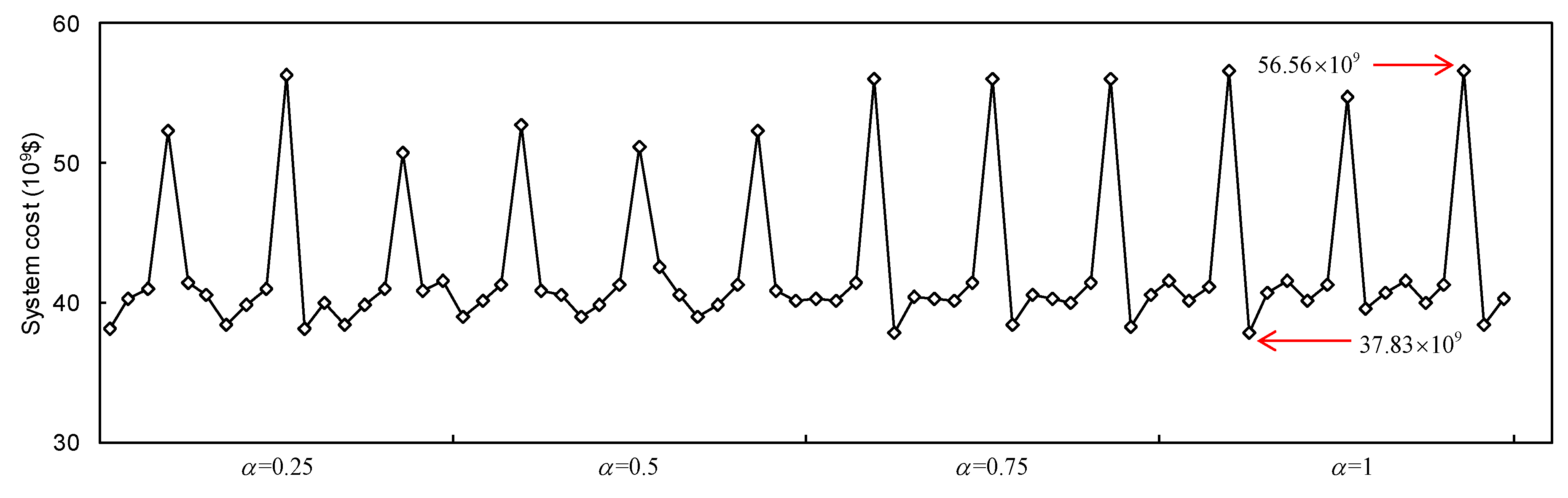
Conversely, when the share of renewable energy accounts for 20%, there has been a downward trend in economic cost under the three levels. The economic cost would be $51.15 × 10⁹, $42.59 × 10⁹, and $40.569 × 10⁹ in period 1, 2, and 3, respectively (when ). The main reason is that more renewable energy installed capacity is needed under the scenario compared with . In general, to effectively increase the sustainable power supply during the planning horizon, the capacity expansions would be implemented sooner rather than later [27]. Therefore, the expansion of renewable energy in the early part of the planning period would result in a significant increase in system costs. However, as the initial capacity-expansion investment ends and the cost of power generation from renewable energy decreases, the system cost would gradually decrease. For example, in period 3, the system cost would be $40.569 × 10⁹ (when ), $40.536 × 10⁹ (when ), and $40.178 × 10⁹ (when ), which is lower than the results obtained from the 15% share scenario ($41.204 × 10⁹, $41.284 × 10⁹, and $41.2 × 10⁹, respectively). Comparing the system costs over the three planning periods in the two scenarios, the increase in the share of renewable energy in energy supply would bring about a decline in the cost of system power generation in the long-run. Similarly, the results under other credible values (i.e., , , and ) can be interpreted. System cost under different levels with a range from $37.83 × 10⁹ to $56.56 × 10⁹ is depicted in Figure 6.
Figure 7 depicts the electricity generation pattern under different and values (when ). Due to its competitive price and high reliability within the study planning horizon, coal-fired electricity supply would account for a large proportion. According to the CV reduction method and generalized credibility measure method, rising the credible value would bring about a decrease in the values of renewable energy availabilities, and increase the values of the export power demand. The results indicate that the shares of wind power and natural gas in total supply would present upward trends by descending the value of . For example, when , wind power would contribute 12.34% (), 12.39% (), 12.44% (), and 12.46% () of the total electricity (see Figure 7a–d), and there would be a similar trend when (see Figure 7e–h). The results of wind power and natural gas would be more sensitive to uncertain inputs than that of coal-fired, photovoltaic, or hydropower. This is because coal-fired, photovoltaic or hydropower accounts for a large or too small share of total power generation, and the change in has limited impact on them. Compared with the scenario, the share of photovoltaic increased significantly in the scenario. To be specific, when , , , and , the share of photovoltaic power generation increased by 3.73%, 3.74%, 2.83%, and 2.72%, respectively. The main reason is that the cost of photovoltaic generation is lower than that of natural gas, and the resource availability of photovoltaic is more than that of hydropower in the study area. Moreover, the initial installed capacity of photovoltaic in the study area is smaller, and the space for expansion is larger than that of wind power.
Figure 8 shows the optimal capacity expansion schemes under different , values and levels (when ). The results indicate that the existing electricity generation capacities would be insufficient for the increasing electricity demands. Differences in the capacity-expansion option for various power generation technologies can be found between the results of the two scenarios (, ). represents the displacement coefficient of renewable energy resource. Hu et al. found that each unit of electricity supplied by renewable energy resources avoids the generation of an equal amount of electricity by traditional fossil-fuel generators, which only occurs in the ideal scenario [34]. The solution considering displacement efficiency coefficient (i.e., ) generally leads to more capacity expansion to meet the end-users demand. When and , more capacity expansion would be conducted in the range of 0.32% to 3% compared to the solutions with ; when and , that would be in the range of 4% to 9%. Comparing the two scenarios with a different displacement coefficient, there was no expansion of PV facilities which would be conducted under different levels (when , ). Conversely, the different capacity expansion would be undertaken on other power generation facilities. Photovoltaic power generation has a high capacity expansion cost and high operating cost, and thus photovoltaic facilities would only be implemented for expansion under some harsh conditions (i.e., when the expansions of other energy generating facilities cannot guarantee power demand). Increased credibility means more stringent environmental constraints which would lead to different expansion schemes to be conducted. For example, when and , with rising from 0.25 to 1, there was an upward trend in the total capacity expansion, being 40.89, 41.49, 41.62, and 42.37 GWh, respectively. Similarly, when and , the total capacity expansion would respectively be 41.02, 41.62, 42.37, and 43.09 GWh. Under scenario, when , the overall trend of the expansion scheme within the planning horizon would be similar to that under scenario. However, when and , total capacity expansion would show an upward trend of volatility. For example, when rise from 0.25 to 1, the total expansion capacity would be 49.64, 49.59, 51.22, and 50.34 GWh, respectively.
Different and levels in optimal power generation schemes illustrate that the results are sensitive to inexact system inputs (see Figure 9). For instance, in period 2, to satisfy local electricity demand, the entire coal-fired electricity generation obtained from the 15% share scenario would be 183.87, 236.28, 220.71, and 241.92 × 10³ GWh for 0.25, 0.5, 0.75, and 1, respectively; the gas-fired power generation would be 55.69, 24.61, 18.11, and 3 × 10³ GWh; the wind power generation would be 53.54, 32.96, 51.34, and 53.54 × 10³ GWh; the PV would be 10.62, 5.06, 8.69, and 0 × 103 GWh; and the hydropower would be 0, 2.05, 4.91, and 4.53 × 10³ GWh. More concretely, PV is most sensitive to changes in but not sensitive to and levels. For example, when , the total PV power generation would be 10.62 × 10³ GWh under different and levels, but when reaches 20%, the total amount of PV would be more than 1.034~1.373 times that of under scenario. When , the coal-fired power generation would increase with the ascending of . For example, when , , with rising from 0.25 to 1, the coal-fired power generation would respectively be 226.879, 227.303, 227.039, 229.965 × 10³ GWh in period 1, 245.694, 245.767, 246.532, 246.779 × 10³ GWh in period 2, and 268.736, 269.832, 271.337, 272.543 × 10³ GWh in period 3; however, when , it presents a trend of slight fluctuation. In addition, coal-fired power generation would also increase with the ascending of the level. For example, when , , corresponding to rise to 0.1, the coal-fired power generation amounts would be 245.694, 246.214, and 246.843 × 10³ GWh in period 2, respectively. Hydropower would be the most sensitive to changes when compared to other power generation technology. For instance, when , corresponding to a rise from 0.25 to 1, the results obtained from hydropower would be 4.88, 6.07, 7.57, and 9.01, respectively. However, the change in level would not affect the hydropower generation. Wind power generation and natural gas power generation are more sensitive to changes in electricity demand than that of the changes in , , and .
Figure 10 exhibits the power generation schemes under two share scenarios (when , , ). The rise in the proportion of renewable energy generation would bring down the percentage of coal-fired electricity generation. For example, when , the local coal-fired power generation would be 701.17 × 10³ GWh, lower than 760.8 × 10³ GWh (when ). Under scenario , PV generation would respectively be 48.16 × 10³ GWh for local and 27.44 × 10³ GWh for export, higher than that under scenario (21.24 × 10³ GWh for local, 10.62 × 10³ GWh for export). In two scenarios, the electricity generation patterns of natural gas power generation, wind power, and hydropower are different, but the total power generations are the same, which would be 175.13 × 10³ GWh, 143.89 × 10³ GWh, and 27.06 × 10³ GWh, respectively. This is the result of the tradeoff between air pollutants emissions and economic costs. Likewise, the results under different values can be similarly analyzed.
In order to demonstrate the superiority of the presented approach compared with previous methods, the optimal-ratio problem (T2FCFP-GEP) proposed in models 13a–14o can be converted into a least-cost problem defined by Equation (15).
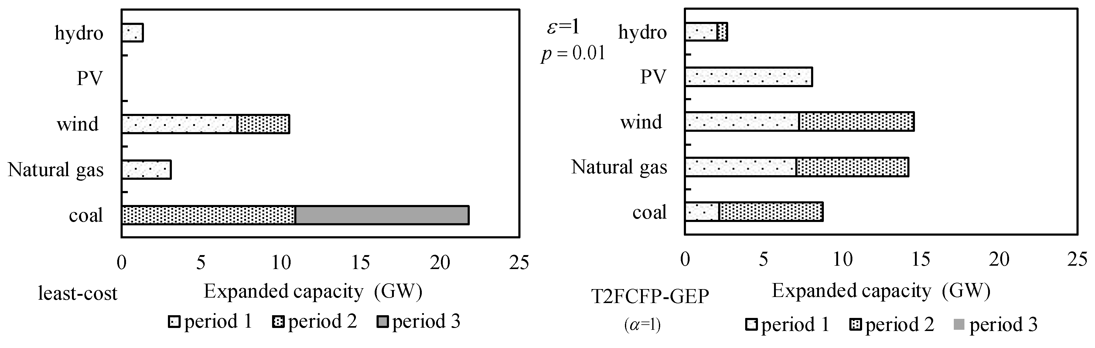
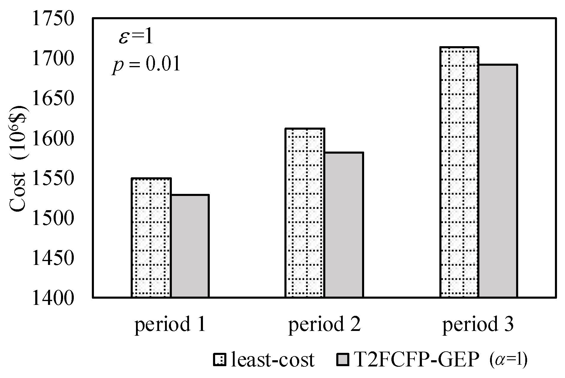
Figure 11 reveals the power generation patterns obtained from T2FCFP-GEP (when ) and least-cost models under scenario. The T2FCFP-GEP model achieves a relatively higher proportion of clean energy generation. According to the results of the two models, the percentage of power generated by clean energy facilities would be 21.6% (least-cost) and 36% (T2FCFP-GEP). In comparison, the least-cost model leads to a slightly higher capacity expansion of coal-fired power generation and lower opportunities for clean energy development (see Figure 12). Take coal-fired facilities as an example (corresponding to ), to meet the growing demand for electricity; the capacity of 2.2 GW and 6.55 GW would be added to the coal-fired facilities in period 1 and period 2 of the T2FCFP model but would not be expanded in period 3. The total expansion capacity during the three planning periods would be lower than the expansion capacity of 10.9 GW in the second planning period of the least-cost model. With another electricity capacity expansion of 10.9 GW in the third planning period, the total coal-fired electricity expansion capacity of the least-cost model would reach 21.8 GW. Similarly, the expansion differences of other electricity facilities can be found between the results of the two models. As illustrated from Figure 13, the cost for pollutant treatment and pollutant emission from T2FCFP-GEP model would be lower than that of the least-cost model. The cost for pollutant treatment and pollutant emission would be $1549.6, $1612.65, and $1713.77 × 106 in the three study periods from the least-cost model, which is higher than the T2FCFP-GEP model, $1528.81, $1591.74, and $1692.07 × 106, respectively. In addition, certainty models have limitations in representing various planning impact factors, such as radical and conservative attitudes of decision-makers, renewable energy availability, etc. In contrast, decision-makers would prefer models that could reflect complex conditions.
4. Conclusions
This study presents a type-2 fuzzy chance-constrained fractional programming (T2FCFP) method for electric power system (EPS) sustainable management under varied forms of uncertainties. This method has shown to be useful for solving dual-objective problems with ratio optimization and uncertainties in varied forms such as probability distributions, type-2 fuzzy sets, and distribution with fuzzy probability. The proposed hybrid T2FCFP method has the following advantages:
(a) The T2FCFP method could balance the dual objectives of minimizing system cost and maximizing clean energy generation, as well as the trade-offs between system efficiency and environmental constraints.
(b) The intermittent characteristics of renewable energy availability parameters could be expressed as type-2 fuzzy variables by the T2FCFP method and quantified as determined model input parameters by the generalized confidence level.
(c) The T2FCFP method could provide plenty of scenario-based results and various decision alternatives with different violation risks, which could help decision-makers identify the impact of different energy policies on electricity generation patterns, expansion schemes, and economic costs. Sensitivity analysis and comparison of results obtained from the alternative schemes could help decision-makers to identify the desired long-term regional energy policies under different system-reliability and economic constraints.
The T2FCFP method has been applied to a case study of the generation expansion planning problem of electric power system in China. Results obtained from the T2FCFP-GEP model are proven to be effective to support decision-making of sustainable management of EPS under both fuzzy and stochastic uncertainties. The results suggest expanding renewable resources development and maintaining clean-energy production would decrease the total system cost and improve energy sustainability. The mix ratio of electricity generation by clean energy in the whole energy supply and the displacement efficiency of power generation technology by renewable energy will have a statistically significant impact on power generation patterns, capacity expansion schemes, and system costs.
This study is the first attempt for tackling electric power system management through the developed T2FCFP-GEP model; the results implied that the developed T2FCFP method was applicable to practical EPS sustainable management problems associated with uncertain and highly complex information. Also, the T2FCFP method could be extended and applied to other energy decision-making problems; for example, pollutant emissions mitigation programming and water resource management.
Author Contributions
The study and the writing of the manuscript were carried out with contributions from all the authors. Writing—original draft preparation, C.Y. and J.C.; methodology, C.Z., J.C., and G.H.
Funding
This research was supported by Fundamental Research Funds for the Central Universities, NCEPU (2017MS030), the National Key Research and Development Plan (2016YFC0502800), the Natural Sciences Foundation (51520105013, 51679087), and the 111 Program (B14008).
Conflicts of Interest
The authors declare no conflict of interest.
Nomenclatures
| Research period, (5-year for each period) | |
| Electricity generation technology, ( coal, natural gas, hydropower, wind power, and photovoltaic) | |
| Type of power demand ( local, export) | |
| Options of capacity expansion, | |
| Type of the air pollutant, ( SO2, NOx, PM) | |
| Supply of primary energy resource for electricity generation technology in period (TJ) | |
| Power generated by electricity generation technology for electric network in period (GWh). | |
| Hydropower availability in period . | |
| Wind energy availability in period | |
| Solar energy availability in period | |
| Cost for expanding the electricity capacity in period (103 $/GW) | |
| Cost for primary energy supply for electricity generation technology in period (103 $/TJ) | |
| Cost for pollution mitigation of electricity generation technology in period (103 $/tonne) | |
| Fixed and variable cost for generating power via technology in period (103 $/GWh) | |
| Cost for transmission and distribution in period (103 $/GWh) | |
| Local power demand in period (GWh) | |
| Export power demand in period (GWh) | |
| Permitted emission of pollutant in period (103 tonne) | |
| Capacity expansion option of electricity generation technology in period (GW) | |
| The rate of electricity transmission line loss in period (%) | |
| Penalty of air pollutant emission of electricity generation technology in period (103 $/tonne) | |
| Air pollution equivalent values in period | |
| Residual capacity of electricity generation technology in period (GW) | |
| Retirement capacity of electricity generation technology in period (GW) | |
| Subsidy for air pollution control from fossil-fired generation technology in period (103 $/GWh) | |
| Subsidy for green energy generation technology in period (103 $/GWh) | |
| Revenue of exported electricity of electricity generation in period (103 $/GWh) | |
| Maximum service time of electricity generation technology in period | |
| Maximum service time of power transmission line in period (hour). | |
| Available primary energy in period (TJ) | |
| Maximum capacity of electricity generation technology in period (GW) | |
| Maximum electric transmission capacity in period | |
| Capacity option for electricity generation technology in period | |
| Emission factor of the air pollutant in period (103 tonne/GWh). | |
| Minimum proportion of electricity generation from renewable energy in the entire energy supply. | |
| Removal efficiency of pollutant for electricity generation technology in period | |
| Conversion factor of electricity generation technology in period (TJ/GWh) | |
| Displacement efficiency coefficient of electricity generation technology in period | |
| Conversion factor of hydropower in period | |
| Conversion factor from wind energy to electricity in period | |
| Conversion factor from solar energy to electricity in period | |
| Constraint-violation probability in period |
References
- Zhang, X.Y.; Huang, G.H.; Zhu, H.; Li, Y.P. A fuzzy-stochastic power system planning model: Reflection of dual objectives and dual uncertainties. Energy 2017, 123, 664–676. [Google Scholar] [CrossRef]
- Li, W.; Bao, Z.; Huang, G.H.; Xie, Y.L. An Inexact Credibility Chance-Constrained Integer Programming for Greenhouse Gas Mitigation Management in Regional Electric Power System under Uncertainty. J. Environ. Inform. 2017, 31, 111–122. [Google Scholar] [CrossRef]
- Bekebrede, G.; van Bueren, E.; Wenzler, I. Towards a joint local energy transition process in urban districts: The go2zero simulation game. Sustainability 2018, 10, 2602. [Google Scholar] [CrossRef]
- Oprea, S.V.; Bâra, A.; Majstrović, G. Aspects Referring Wind Energy Integration from the Power System Point of View in the Region of Southeast Europe. Study Case of Romania. Energies 2018, 11, 251. [Google Scholar] [CrossRef]
- Koltsaklis, N.E.; Liu, P.; Georgiadis, M.C. An integrated stochastic multi-regional long-term energy planning model incorporating autonomous power systems and demand response. Energy 2015, 82, 865–888. [Google Scholar] [CrossRef]
- López, J.; Pozo, D.; Contreras, J.; Mantovani, J.R.S. A convex chance-constrained model for reactive power planning. Int. J. Electr. Power Energy Syst. 2015, 71, 403–411. [Google Scholar] [CrossRef] [Green Version]
- Cai, Y.P.; Huang, G.H.; Yang, Z.F.; Tan, Q. Identification of optimal strategies for energy management systems planning under multiple uncertainties. Appl. Energy 2009, 86, 480–495. [Google Scholar] [CrossRef]
- Huang, G.H. A hybrid inexact-stochastic water management model. Eur. J. Oper. Res. 1998, 107, 137–158. [Google Scholar] [CrossRef]
- Huang, G.H.; Loucks, D.P. An inexact two-stage stochastic programming model for water resources management under uncertainty. Civ. Eng. Syst. 2000, 17, 95–118. [Google Scholar] [CrossRef]
- Li, Y.F.; Li, Y.P.; Huang, G.H.; Chen, X. Energy and environmental systems planning under uncertainty—an inexact fuzzy-stochastic programming approach. Appl. Energy 2010, 87, 3189–3211. [Google Scholar] [CrossRef]
- Guo, X.; Bao, Z.; Li, Z.; Yan, W. Adaptively Constrained Stochastic Model Predictive Control for the Optimal Dispatch of Microgrid. Energies 2018, 11, 243. [Google Scholar] [CrossRef]
- Hu, J.; Sun, L.; Li, C.H.; Wang, X.; Jia, X.L.; Cai, Y.P. Water Quality Risk Assessment for the Laoguanhe River of China Using a Stochastic Simulation Method. J. Environ. Inform. 2018, 31, 123–136. [Google Scholar] [CrossRef]
- Li, Y.; Yang, Z.; Li, G.; Zhao, D.; Tian, W. Optimal scheduling of an isolated microgrid with battery storage considering load and renewable generation uncertainties. IEEE Trans. Ind. Electron. 2019, 66, 1565–1575. [Google Scholar] [CrossRef]
- Zhou, Y.; Li, Y.P.; Huang, G.H. Integrated modeling approach for sustainable municipal energy system planning and management–a case study of Shenzhen, China. J. Clean. Prod. 2014, 75, 143–156. [Google Scholar] [CrossRef]
- Suo, C.; Li, Y.P.; Wang, C.X.; Yu, L. A type-2 fuzzy chance-constrained programming method for planning Shanghai’s energy system. Int. J. Electr. Power Energy Syst. 2017, 90, 37–53. [Google Scholar] [CrossRef]
- Chen, B.; Li, P.; Wu, H.J.; Husain, T.; Khan, F. MCFP: A Monte Carlo Simulation-based Fuzzy Programming Approach for Optimization under Dual Uncertainties of Possibility and Continuous Probability. J. Environ. Inform. 2017, 29, 88–97. [Google Scholar] [CrossRef]
- Zhou, Y.; Li, Y.P.; Huang, G.H. Planning sustainable electric-power system with carbon emission abatement through CDM under uncertainty. Appl. Energy 2015, 140, 350–364. [Google Scholar] [CrossRef]
- Rekik, M.; Abdelkafi, A.; Krichen, L. A micro-grid ensuring multi-objective control strategy of a power electrical system for quality improvement. Energy 2015, 88, 351–363. [Google Scholar] [CrossRef]
- Azadeh, A.; Raoofi, Z.; Zarrin, M. A multi-objective fuzzy linear programming model for optimization of natural gas supply chain through a greenhouse gas reduction approach. J. Nat. Gas Sci. Eng. 2015, 26, 702–710. [Google Scholar] [CrossRef]
- Li, K.; Pan, L.; Xue, W.; Jiang, H.; Mao, H. Multi-objective optimization for energy performance improvement of residential buildings: A comparative study. Energies 2017, 10, 245. [Google Scholar] [CrossRef]
- Cui, Y.; Geng, Z.; Zhu, Q.; Han, Y. Multi-objective optimization methods and application in energy saving. Energy 2017, 125, 681–704. [Google Scholar] [CrossRef]
- Harkouss, F.; Fardoun, F.; Biwole, P.H. Multi-objective decision making optimization of a residential net zero energy building in cold climate. In Proceedings of the 2017 Sensors Networks Smart and Emerging Technologies (SENSET), Beirut, Lebanon, 12–14 September 2017; pp. 1–4. [Google Scholar]
- Jahromi, M.E.; Ehsan, M.; Meyabadi, A.F. A dynamic fuzzy interactive approach for DG expansion planning. Int. J. Electr. Power Energy Syst. 2012, 43, 1094–1105. [Google Scholar] [CrossRef]
- Li, Y.; Wang, J.; Zhao, D.; Li, G.; Chen, C. A two-stage approach for combined heat and power economic emission dispatch: Combining multi-objective optimization with integrated decision making. Energy 2018, 162, 237–254. [Google Scholar] [CrossRef] [Green Version]
- Nie, S.; Huang, C.Z.; Huang, G.H.; Li, Y.P.; Chen, J.P.; Fan, Y.R.; Cheng, G.H. Planning renewable energy in electric power system for sustainable development under uncertainty—A case study of Beijing. Appl. Energy 2016, 162, 772–786. [Google Scholar] [CrossRef]
- Wang, L.; Huang, G.; Wang, X.; Zhu, H. Risk-based electric power system planning for climate change mitigation through multi-stage joint-probabilistic left-hand-side chance-constrained fractional programming: A Canadian case study. Renew. Sustain. Energy Rev. 2018, 82, 1056–1067. [Google Scholar] [CrossRef]
- Zhu, H.; Huang, G.H. Dynamic stochastic fractional programming for sustainable management of electric power systems. Int. J. Electr. Power Energy Syst. 2013, 53, 553–563. [Google Scholar] [CrossRef]
- Zhu, H.; Huang, W.W.; Huang, G.H. Planning of regional energy systems: An inexact mixed-integer fractional programming model. Appl. Energy 2014, 113, 500–514. [Google Scholar] [CrossRef]
- Charnes, A.; Cooper, W.W. Programming with linear fractional functionals. Nav. Res. Logist. Q. 1962, 9, 181–186. [Google Scholar] [CrossRef]
- Mendel, J.M.; John, R.B. Type-2 fuzzy sets made simple. IEEE Trans. Fuzzy Syst. 2002, 10, 117–127. [Google Scholar] [CrossRef]
- Kundu, P.; Kar, S.; Maiti, M. Fixed charge transportation problem with type-2 fuzzy variables. Inf. Sci. 2014, 255, 170–186. [Google Scholar] [CrossRef]
- Liu, Z.Q.; Liu, Y.K. Type-2 fuzzy variables and their arithmetic. Soft Comput. 2010, 14, 729–747. [Google Scholar] [CrossRef]
- Qin, R.; Liu, Y.K.; Liu, Z.Q. Methods of critical value reduction for type-2 fuzzy variables and their applications. J. Comput. Appl. Math. 2011, 235, 1454–1481. [Google Scholar] [CrossRef]
- Zhou, C.; Huang, G.; Chen, J. A Multi-Objective Energy and Environmental Systems Planning Model: Management of Uncertainties and Risks for Shanxi Province, China. Energies 2018, 11, 2723. [Google Scholar] [CrossRef]
- Cheng, C.B. Group opinion aggregation based on a grading process: A method for constructing triangular fuzzy numbers. Comput. Math. Appl. 2004, 48, 1619–1632. [Google Scholar] [CrossRef]
- Liu, B.; Iwamura, K. Chance constrained programming with fuzzy parameters. Fuzzy Sets Syst. 1998, 94, 227–237. [Google Scholar] [CrossRef]
- Hu, Y.; Cheng, H. Displacement efficiency of alternative energy and trans-provincial imported electricity in China. Nat. Commun. 2017, 8, 14590. [Google Scholar] [CrossRef] [PubMed] [Green Version]
- Statistics Bureau of Shanxi Province. Shan Xi Statistical Yearbook in 1994–2017; China Statistical Press: Shanxi, China, 1994–2017. (In Chinese)
Figure 1.
Defuzzification process of the type-2 fuzzy variable (T2FV).

Figure 2.
Distribution of electricity installed capacity in the Province of Shanxi, China in 2017.

Figure 3.
Power consumption of Shanxi, China (1999–2016).

Figure 4.
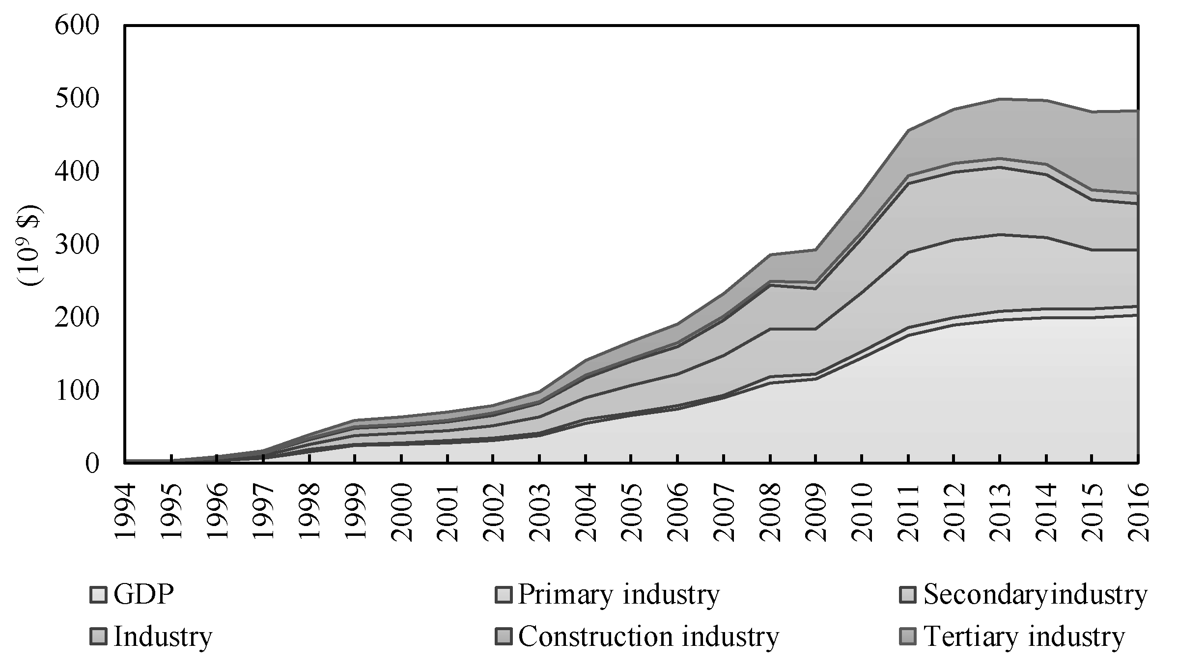
The relevant economic parameters for electricity demand forecasting.

Figure 5.
Economic cost under different levels and values.

Figure 6.
System cost under different levels.

Figure 7.
Comparison of power-generation patterns. Note. (a–d): ; (e–h): .

Figure 8.
Capacity expansion schemes under different , values and levels.

Figure 9.
Power generations under different and levels. Note. (a–c): ; (d–f): .

Figure 10.
Comparison of power generations under two share scenarios. Note: L: local; E: export.

Figure 11.
Comparison of power generation patterns from T2FCFP-GEP and least-cost models.

Figure 12.
Comparison of capacity expansions from two models.

Figure 13.
Comparison of total cost for pollutant treatment and pollutant emission from two models.


Table 1.
Primary energy supply cost and emission cost.
| Primary Energy | Air Pollutants | Period | ||
|---|---|---|---|---|
| t = 1 | t = 2 | t = 3 | ||
| Energy supply cost (103 $/TJ) | ||||
| Coal | 3.96 | 4.554 | 5.237 | |
| Natural gas | 6.76 | 7.436 | 8.18 | |
| Emission cost ($/tonne) | ||||
| SO2 | 99 | 108.9 | 119.79 | |
| NOx | 99 | 108.9 | 119.79 | |
| PM | 23 | 25.3 | 27.83 | |
Table 2.
Power generation technical parameters.
| Electricity-Generation Technology | Electricity Generation Cost (103 $/GWh) | Installed Capacity (GW) |
|---|---|---|
| Coal | 32.77 | 59.43 |
| NG | 44.82 | 3.88 |
| Wind | 36.47 | 8.72 |
| PV | 40.31 | 5.90 |
| Hydro | 21.50 | 2.44 |
Note. Coal: coal-fired power; NG: natural gas; Wind: wind; PV: photovoltaic; Hydro: hydropower.
Table 3.
Expansion options and expansion costs for electricity generation facilities.
| Electricity-Generation Technology | Options | Period | ||
|---|---|---|---|---|
| t = 1 | t = 2 | t = 3 | ||
| Capacity expansion options (GW) | ||||
| Coal | m = 1 | 2.2 | 2.2 | 2.2 |
| m = 2 | 6.55 | 6.55 | 6.55 | |
| m = 3 | 10.9 | 10.9 | 10.9 | |
| NG | m = 1 | 3.12 | 3.12 | 3.12 |
| m = 2 | 5.12 | 5.12 | 5.12 | |
| m = 3 | 7.12 | 7.12 | 7.12 | |
| Wind | m = 1 | 5.28 | 5.28 | 5.28 |
| m = 2 | 6.28 | 6.28 | 6.28 | |
| m = 3 | 7.28 | 7.28 | 7.28 | |
| PV | m = 1 | 4.1 | 4.1 | 4.1 |
| m = 2 | 6.1 | 6.1 | 6.1 | |
| m = 3 | 8.1 | 8.1 | 8.1 | |
| Hydro | m = 1 | 0.6 | 0.6 | 0.6 |
| m = 2 | 1.35 | 1.35 | 1.35 | |
| m = 3 | 2.07 | 2.07 | 2.07 | |
| Capacity expansion cost (106 $/GW) | ||||
| Coal | 577 | 547 | 517 | |
| NG | 726 | 686 | 646 | |
| Wind | 1256 | 1156 | 1056 | |
| PV | 1877 | 1677 | 1477 | |
| Hydro | 1597 | 1497 | 1397 | |
© 2019 by the authors. Licensee MDPI, Basel, Switzerland. This article is an open access article distributed under the terms and conditions of the Creative Commons Attribution (CC BY) license (http://creativecommons.org/licenses/by/4.0/).
Share and Cite
MDPI and ACS Style
Zhou, C.; Huang, G.; Chen, J. A Type-2 Fuzzy Chance-Constrained Fractional Integrated Modeling Method for Energy System Management of Uncertainties and Risks. Energies 2019, 12, 2472. https://doi.org/10.3390/en12132472
AMA Style
Zhou C, Huang G, Chen J. A Type-2 Fuzzy Chance-Constrained Fractional Integrated Modeling Method for Energy System Management of Uncertainties and Risks. Energies. 2019; 12(13):2472. https://doi.org/10.3390/en12132472
Chicago/Turabian StyleZhou, Changyu, Guohe Huang, and Jiapei Chen. 2019. "A Type-2 Fuzzy Chance-Constrained Fractional Integrated Modeling Method for Energy System Management of Uncertainties and Risks" Energies 12, no. 13: 2472. https://doi.org/10.3390/en12132472
Note that from the first issue of 2016, this journal uses article numbers instead of page numbers. See further details here.