Deep Learning with Stacked Denoising Auto-Encoder for Short-Term Electric Load Forecasting

Yangzhong Intelligent Electrical Institute, North China Electric Power University, Yangzhong 212200, China
*
Author to whom correspondence should be addressed.
Energies 2019, 12(12), 2445; https://doi.org/10.3390/en12122445
Submission received: 24 May 2019
/
Revised: 6 June 2019
/
Accepted: 10 June 2019
/
Published: 25 June 2019
(This article belongs to the Special Issue Selected papers from the Fourth IEEE International Symposium on Computer, Consumer and Control, 2018 (IS3C 2018))
Abstract
:Accurate short-term electric load forecasting is significant for the smart grid. It can reduce electric power consumption and ensure the balance between power supply and demand. In this paper, the Stacked Denoising Auto-Encoder (SDAE) is adopted for short-term load forecasting using four factors: historical loads, somatosensory temperature, relative humidity, and daily average loads. The daily average loads act as the baseline in final forecasting tasks. Firstly, the Denoising Auto-Encoder (DAE) is pre-trained. In the symmetric DAE, there are three layers: the input layer, the hidden layer, and the output layer where the hidden layer is the symmetric axis. The input layer and the hidden layer construct the encoding part while the hidden layer and the output layer construct the decoding part. After that, all DAEs are stacked together for fine-tuning. In addition, in the encoding part of each DAE, the weight values and hidden layer values are combined with the original input layer values to establish an SDAE network for load forecasting. Compared with the traditional Back Propagation (BP) neural network and Auto-Encoder, the prediction error decreases from 3.66% and 6.16% to 2.88%. Therefore, the SDAE-based model performs well compared with traditional methods as a new method for short-term electric load forecasting in Chinese cities.
1. Introduction
The stability of the electric power system is guaranteed by the balance between electric load and supply. Since electric load values are influenced by many uncertain factors including weather conditions and users’ electric consumption behaviors, electric load forecasting based on these factors is significant [1]. With the help of an accurate electric load forecasting, electric power operators can adjust the electric supply according to real-time forecast load values and maintain the normal operation of electric power systems. Recently, the development of a smart grid makes load forecasting increasingly important [2]. In a smart grid, power distribution department relies on load forecasting to implement electric price fluctuations and demand response strategies [3]. Generally, load forecasting can be classified into four categories: long-term forecasting, medium-term forecasting, short-term forecasting and ultra-short-forecasting. Among them, short-term forecasting is the most widely used in electric power systems. In this paper, short-term load forecasting is discussed.
Short-term load forecasting has drawn attention from a wide range of researchers in various fields and many forecasting methods have been proposed. In general, these forecasting methods consist of two categories: data-driven methods and machine learning methods. The traditional data-driven methods based on time series analysis include the multiple linear regression model [4], the autoregressive integrated moving average model (ARIMA) [5], and the exponentially weighted method [6], etc. However, data-driven methods perform poorly when identifying nonlinearity of electric loads because they’re based on the assumption that electric loads change linearly. With the development of artificial intelligence techniques, machine learning methods with strong nonlinear fitting capability were designed to better reflect the nonlinear features of electric loads.
Machine learning methods, including artificial neural network (ANN), random forest (RF) and support vector regression (SVR) have been widely used to predict the change of electric loads. Huang et al. proposed a new RF-based feature selection method in which an original RF model was trained using an original feature set consisting of 243 related features and then an improved RF model was trained using features selected by a sequential backward search method [7]. The authors in [8] constructed a hybrid prediction model by combining a RF model and a multilayer perceptron (MLP) model to predict the daily electric loads. In [9], the SVR was used to build a strategic, seasonality-adjusted model for electric load forecasting, which can effectively reduce the operator interaction. Nevertheless, although traditional machine learning forecasting methods perform better than data-driven forecasting methods, they entail manual feature extraction and selection which are complicated and time-consuming. On top of that, they cannot deal with large amounts of data. Therefore, deep machine learning was proposed to overcome these problems.
Unlike traditional machine learning, deep machine learning extracts features directly from data. Its forecasting performance is proportional to the scale of data. The deep neural network (DNN) is an enhanced version of the traditional shallow ANN. DNNs increase the depth of ANNs by adding multiple hidden layers between the input layer and the output layer. More layers enable DNNs to fit complex functions with fewer parameters and improve the accuracy of predicting electric load. Merkel et al. compared the effectiveness of various forecasting methods, including a linear regression (LR) model, a shallow ANN and two DNNs with different sizes, and proved that, in general, the DNN outperforms other methods [10]. In addition, it can be concluded that the a large DNN marginally outperforms a small DNN. Hossen et al. applied the DNN on the TensorFlow deep learning platform to predict short-term load and achieved preliminary success [11]. Different Activation functions adjusting weights were used including sigmoid function, rectified linear unit and exponential linear unit. An exponential linear unit was proved to be the most effective one. However, DNNs cannot model changes in time series and the chronological order of sample data is significant in load forecasting. The recurrent neural network (RNN), which is a variation of the traditional DNN, was invented to make up for this defect.
An RNN uses sequential information where the output depends on both the current inputs and the previous inputs. Therefore, it can exhibit temporal dynamic behaviors [12]. RNNs have been employed and proved successful in various fields including speech recognition [13,14], robot control [15], language learning [16] and so on. In addition, RNNs perform well when predicting electric load changes. In [17], the RNN was applied to obtain the load correction. Then, the correction was added to the selected similar day’s data to generate the forecast load information. The authors in [18] implemented a pooling deep RNN which batched a group of customers’ load profiles into a pool of inputs and tackled the over-fitting problem by increasing data diversity and volume. However, the RNN has a fatal flaw: when the number of layers increases, the problems of vanishing and exploding gradient occur. Therefore, the RNN can only go back to a few time steps. Long Short-Term Memory (LSTM), which is a variation of RNN, was designed to overcome the vanishing gradient problem [19].
An LSTM unit contains a memory cell, an input gate, an output gate and a forget gate. When a piece of information enters the LSTM, the cell decides whether the information should be remembered or forgotten according to algorithmic rules. LSTM units keep gradients unchanged to avoid the problem of vanishing gradients. Wei et al. offered solid reasons for choosing LSTM and applied LSTM to predict residential electric load [20]. In [21], Tian et al. designed a novel model combining LSTM and convolutional neural networks (CNN). In this model, the LSTM was used to learn the useful information for a long time and capture the long-term dependency. Then, the hidden features of LSTM together with those of CNN were integrated in the feature-fusion module to make the final prediction. Similarly, Kim et al. proposed a hybrid forecasting model using the LSTM and the CNN [22]. What made this model different from Tian’s is that Kim used multi-LSTM layers to extract features from input sequence, and then fed feature sets to a CNN layer to form an n-day profile. The authors in [23] utilized the LSTM to establish a model considering a probabilistic load forecasting scenario in terms of quantiles. Salah Bouktif et al. improved LSTM by using multiple sequences of relevant inputs time lags to incorporate periodicity characteristics of the electric load [24]. It turned out that the multi-sequence LSTM performs better than single-sequence LSTM.
The gated recurrent units (GRUs), invented by Cho et al. [25], is a variation of the LSTM. A GRU simplifies the structure of a LSTM by combining the forgot gate and the input gate into a single update gate. Due to a simpler structure, a GRU can reduce training time when training large amounts of data. Ugurlu et al. built a three-layer GRU model and proved that this model outperformed all other neural networks and state-of-the-art statistical techniques [25]. In [26], the GRU was used to train selected group and the average of the GRU’s outputs served as forecasting results.
The auto-encoder (AE) is a type of artificial neural network, which can learn efficient data coding using an unsupervised manner. An auto-encoder can find common features from unlabeled data and classify data after training. However, the AE doesn’t perform well when data samples are very different. Therefore, the denoising auto-encoder was invented to enable the neural network to learn features from noisy data by adding noise to input data [27]. The stacked denoising autoencoder (SDAE) is an enhanced version of the DAE, which stacks a multiple denoising auto-encoder together. Compared with shallow neural networks, deep neural networks with multiple nonlinear hidden layers such as SDAEs can learn more complex relationships between input layers and output layers. High-level layers can learn features from lower layers and obtain higher-order and more abstract expressions of inputs [28]. Recently, the SDAE has been used in various fields such as image denoising [29], human activity recognition [30], and feature representation [31].
This paper proposes a novel short-term load forecasting model using an SDAE model. In previous works, random initialization was used to initialize parameters, which causes the following problems: (1) Random initialization makes some weights very small which will easily cause the gradient vanishing; (2) Random initialization increases the error range of initial weights and final weights, which leads to local optimal solutions. In this paper, layer-by-layer pre-training is used to replace random initialization and avoid these problems. Additionally, the model in this paper uses unsupervised learning manner, which reduces human involvement. Data from the Chinese city Fuyang are used to prove the superiority of the model.
The rest of this paper is structured as follows: in Section 2, the background of electric load forecasting is discussed; in Section 3, the SDAE deep neural network is introduced; in Section 4, an SDAE-based model is proposed and its forecasting results are shown; in Section 5, conclusions and future work are presented.
2. Electric Load Forecasting System
Original data are simply classified to obtain a set of analyzed data. Then, these data are analyzed by different methods based on their types. Two types of models are usually used to analyze single-dimensional electric load data and transdimensional electric load data respectively. In a traditional field of electric load forecasting, data are collected and then processed usually by the following methods:
2.1. Single Parameter Electric Load Forecasting Model
A single parameter electric load model mainly focuses on estimating future electric load values based on previous single-dimensional electric load data (such as unary linear regression model, time series prediction model, etc.).
2.2. Transdimensional Electric Load Forecasting Model
In the trans-dimensional load forecasting model, the external data, such as holidays, temperature and humidity, etc., are used for electrical load forecasting analysis. The external data are grouped and aggregated at the beginning of the data pre-processing. For a single dimension, the data of other dimensions can be analyzed to obtain the corresponding results (usually correlation analysis), and then be put into the calculation of the current dimension. The algorithmic idea of this paper is to analyze a single parameter (electric load) using cross-dimensional parameters such as somatosensory temperature, relative humidity, and daily average power load.
3. SDAE Neural Netwok
3.1. Auto-Encoder
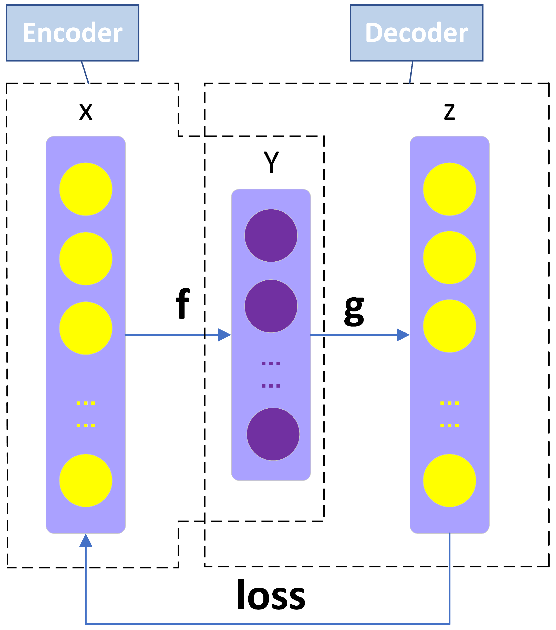
As shown in Figure 1, an auto-encoder is a neural network that uses a backpropagation algorithm to make the output values as equal as possible to the input values. An AE consists of three layers: the input layer x, the hidden layer y, and the output layer z. It compresses the input data x into the hidden layer y to form a higher representation. After the compression, the number of neurons of the hidden layer should be smaller than that of the input layer and the output layer. In this way, the higher representation can be more valuable and the network can learn the hidden features of the input data. Then, the AE reconstructs the input layer data x to obtain output layer data z using the higher representation. The whole learning process is unsupervised [31]. An AE can be divided into two parts: an encoder represented by the function and a decoder that generates the reconstruction . The encoder contains an input layer and a hidden layer, where the original data (set to x) is weighted and mapped to obtain a deterministic map y:
where s is an activation function(sigmoid), x is an input matrix, W is an encoder’s weight matrix and b is an m-dimensional offset vector. The function of the encoder is to compress higher-level data into lower-level data. The decoder consists of a hidden layer and an output layer. Y is inversely mapped to obtain z:
where is an activation function(linear), W′ is the reconstruction decoder′s weights matrix and b′ is the reconstruction m-dimensional offset vector. The function of the decoder is to reconstruct low-level data. Finally, in order to make the input values and the output values as equal as possible, the two sets (W, b) and (W′, b′) are iterated aiming at minimizing the reconstruction error L(x, z). The reconstruction error of AE is defined as:
It should be noted that, if the input data are completely random (for example, each input value is an independent and identically distributed Gaussian random variable that has no connections with other features.), it is very difficult to obtain the relationship between these data. Otherwise, the self-encoding algorithm can discover the relationships between such data and extract the hidden features from them.
3.2. Denoising Auto-Encoder(DAE) and Stacked Denoising Auto-Encoder (SDAE)
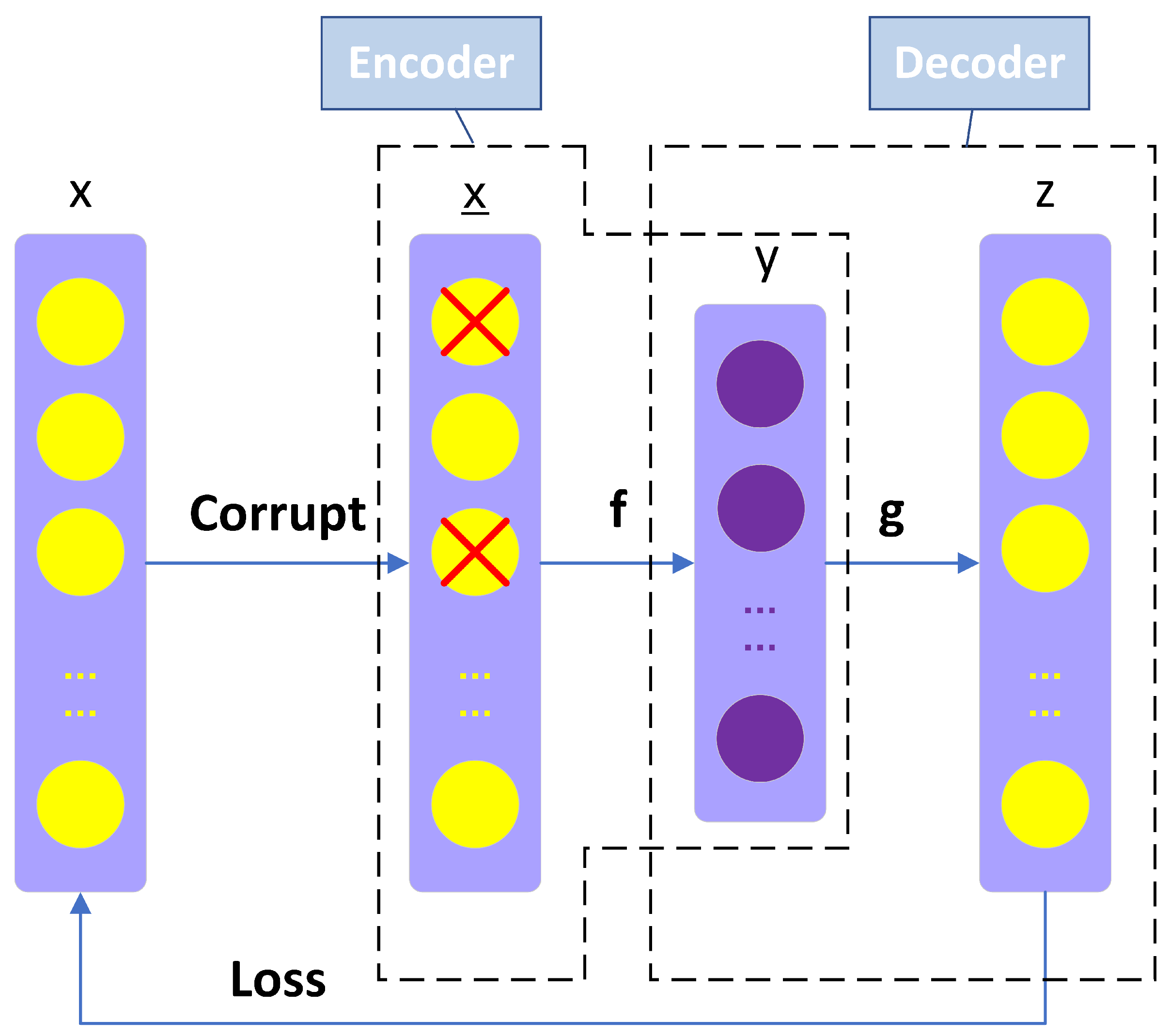
When an AE contains a large number of hidden layer neurons, although the calculation accuracy can be improved, the training time will be longer, the convergence speed will be slow, the over-fitting problem will occur, and the model may only learn the repeated representation of the original data. In order to overcome these problems, Vincent [27] proposed the SDAE model, which is a stack of single-layer DAE. Based on the AE, a Denoising Auto-Encoder (DAE) corrupts the input data to prevent the over-fitting problem. Compared with the AE, a DAE aims to reconstruct the corrupted input data. Figure 2 shows the structure of the DAE. The corruption progress is to corrupt the input data x (x obeys the normal distribution) in specific proportions. After that, the corrupted data are compressed and reconstructed to make the input data approximate to the output data. If the DAE can restore original data using partially missing data, it can be safely concluded that the hidden layer has captured the potential features of the input layer and original data distribution. The stochastic gradient descent algorithm is used to update weights to minimize the error. The features extracted by a DAE are robust and the generalization ability of the model has been improved. The process of corruption is only used during training of a single DAE, and will not be used after the training is completed.
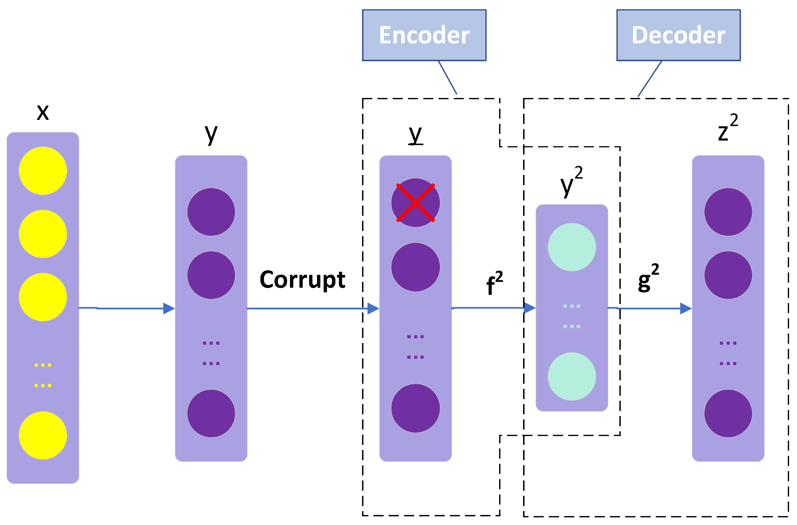
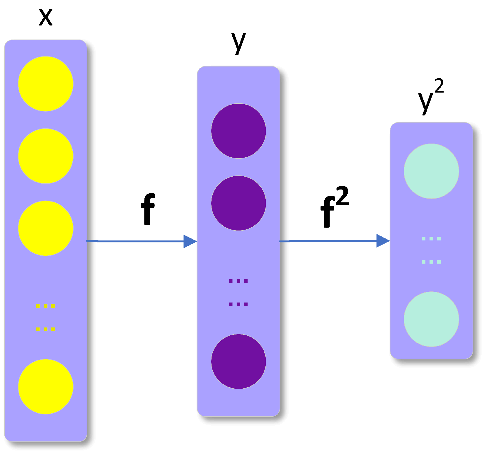
However, in many training tasks, shallow network (such as DAE) capabilities are limited and often do not perform well compared with DNNs. An SDAE is a deep network stacked by multiple DAEs, which can be considered as a type of multilayer perceptron (MLP). In the beginning, original input data are used to generate higher representation. Next, the hidden layer of the first trained DAE is taken out as the input of the next DAE to extract higher representations.
3.3. SDAE Model
An SDAE with an unsupervised pre-training process is firstly used to establish the electric load forecasting model. In this paper, the training process of the entire network is divided into two phases: unsupervised pre-training and supervised fine-tuning. In the unsupervised pre-training process, the unsupervised pre-training is effective to prevent the over-fitting problem in developing a DNN model [32]. Each DAE is trained iteratively layer by layer. Then, the weights of encoder part w and hidden layer values y are combined with original input values x to form a four-layer SDAE network, including an input layer, two hidden layers, and an output layer. It should be noted that the hidden layer neurons of the third trained DAE directly serve as the output values of the entire network. It is different from other studies using SDAE for forecasting tasks [33,34,35,36,37,38] where a new input layer is added to models to extract features of input data. At the top level, a prediction layer is put into the model to complete the prediction task. In the fine-tuning process, the complete network is further trained to minimize the error based on the actual and forecast load values.
During the training process:
- Raw data are standardized in data preprocessing.
- Greedy layer-wise pre-training is used on the parameters of the entire network to pre-train the network [31]. By using the SDAE, the initial weight values and initial offset values of the whole neural network are obtained, and the weight error range of the fine-tuning process is reduced [32], effectively avoiding over-fitting and gradient vanishing in our research.
- The early-stop method is also used to prevent overfitting. This strategy is widely used in traditional machine learning. It is currently the simplest and most effective way, and it is better than the regularization method in many cases.
- The performance of the network is highly dependent on the number of layers in the hidden layer and the number of neurons in each layer. Therefore, we use the fit_generator function in the code that forms the network.
- Parameters W and b are updated by using the gradient descent method.
- In each layer, hidden units = 400, dropout = 10%, epoch = 20, encoder activation function = sigmoid, decoder activation function = linear, loss function = MSE, batch = 20.
3.4. Experiment Process
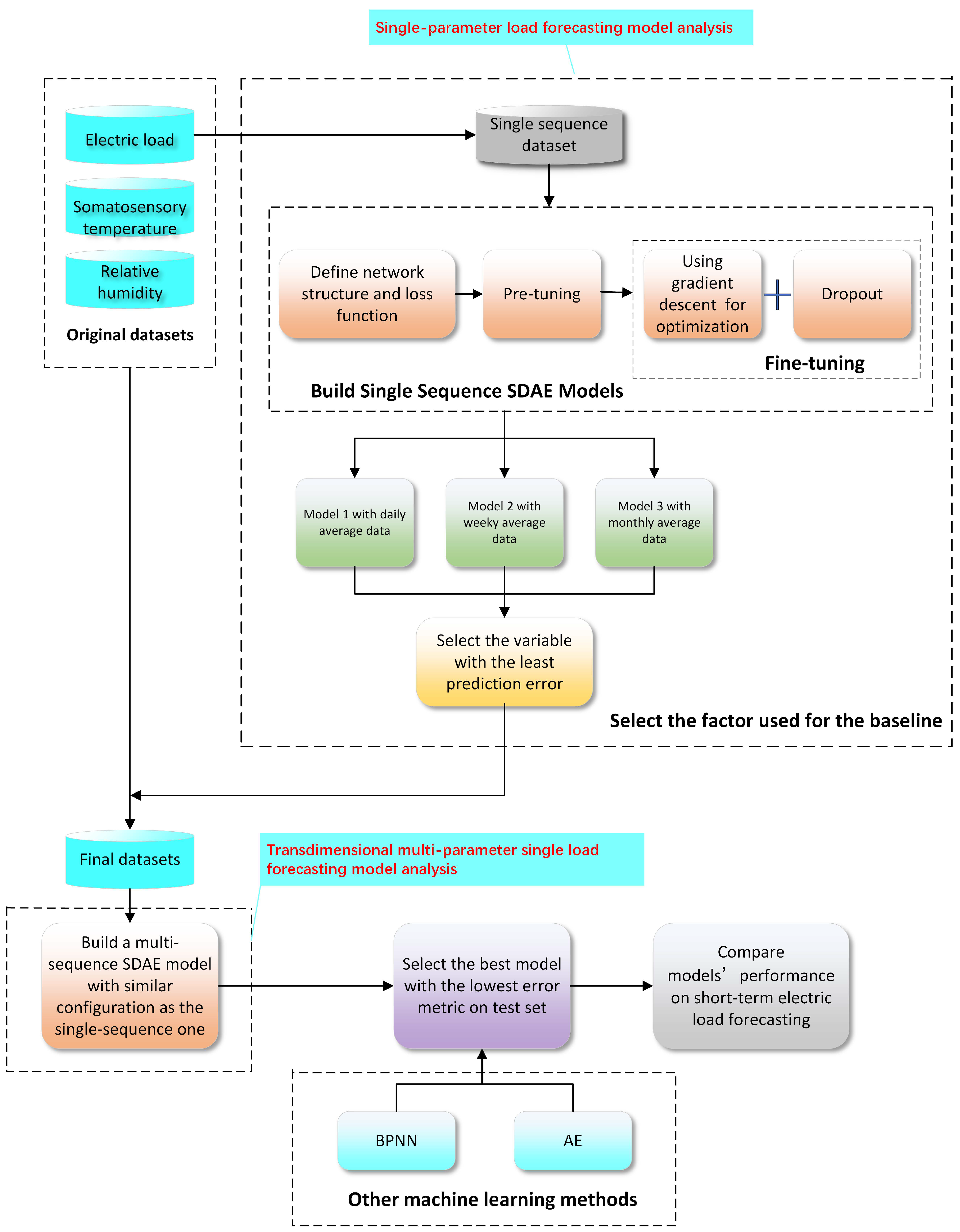
Based on the traditional single-parameter electric load model analysis method, the result of analyzing, modeling and predicting a single parameter has the relevance consistency, which leads to two problems. The first is that the data with weak correlations have a high proportion in the prediction process. The second is that the data with strong correlations have a low proportion in the prediction process. Therefore, multi-dimensional data need to be used for combined correlation analysis. The process of single-parameter load model analysis in multi-dimensions based on the SDAE is as follows:
- Step 1: Collect the electric load data to construct a training datasets matrix, where the data dimensions include historical electric load data, somatosensory temperature data, and relative humidity data.
- Step 2: Respectively calculate the daily average, weekly average and monthly average of historical electric load data and form three single-sequence datasets.
- Step 3: Input the three datasets into their respective SDAE network models, and set each correlation coefficient to obtain the daily average data weight matrix Wd and the corresponding paranoid item Bd, the weekly average data weight matrix Ww and the corresponding paranoid item Bw, the monthly average data weight matrix Wm, and the corresponding paranoid item Bm.
- Step 4: Respectively execute the forward algorithm and the backpropagation algorithm to optimize the parameters of the electric load model. Then, find the average load values with the smallest forecasting error as the fourth factor of the whole dataset to form a new training dataset which is input into the SDAE network model.
- Step 5: Minimize the cost of each neuron by multiple debugging to obtain a well-trained SDAE network model.
- Step 6: Import the previously prepared test data, input the original data into the well-trained SDAE model, and obtain the test result by iteration.
- Step 7: Compare the predicted values with the actual values and calculate the average error.
A schematic diagram of the model is shown in Figure 5:
4. Case Study
4.1. Data Descriptions
In the experiment, the proposed model is trained using electric load data of a city in southern China. Electric load data are sampled every 15 min and the time interval is 15 min (i.e., 96 data points per day). The trend extrapolation adopted in this paper uses the information of historical data to find the trend of historical load changes based on SDAE unsupervised algorithm. In the forecasting task, the future load values are extrapolated according to this trend. The hold-out method is used to validate the forecasting performance in this paper. The hold-out method is a validation method, which divides the original datasets into training datasets and testing datasets. The training datasets are used to train the model and the testing datasets are used to test the model performance. The proportion of training datasets should be more than 70%. Due to the limitation of data, the proportion of training datasets in this paper is set as 90% to make it as large as possible. Therefore, data from 1 January 2013 to 30 September 2013 constitute the training datasets and data from 1 October 2013 to 31 October constitute the forecasting datasets.
Actually, the electric load data are affected by many factors. In this paper, two weather factors are selected: somatosensory temperature and relative humidity. The historical data of these factors are obtained from the Historical Weather Data [39].
In data pre-processing, raw data are standardized by the following equation:
4.2. Forecasting Performance Metrics
Three criteria are used to evaluate the performance of each method. They are the mean absolute error (MAE), mean absolute percentage error (MAPE), root mean-squared error (RMSE), and mean-squared error, which are computed respectively as follows:
where preal and ppre represent measured value and predictive value of the electric data. N denotes the total number of samples used for performance evaluation.
4.3. Load Forecasting
4.3.1. The Selection of the Fourth Factor
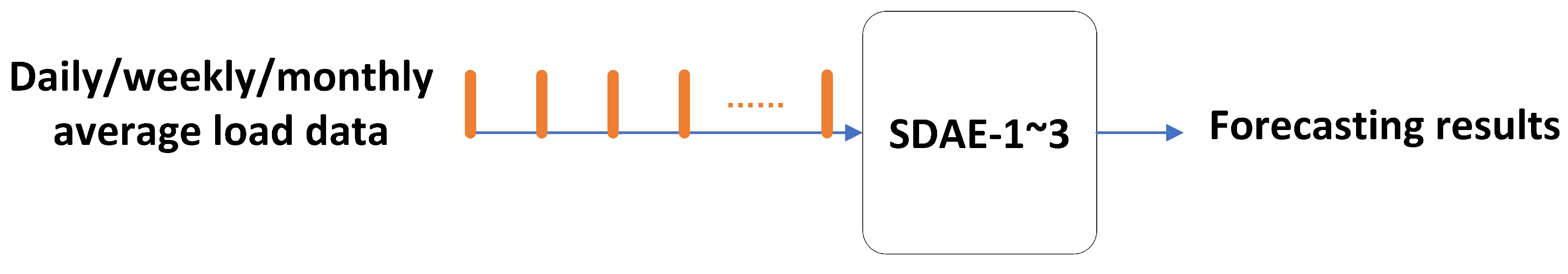
Electric loads have obvious changing trends, which are characterized by periodicity, seasonality, timeliness, and so on. In terms of periodicity, there exist several main change characteristics: (1) Change laws between different days are roughly similar; (2) Change laws of the week type with the same number of days are consistent; and (3) Change laws between holidays and workdays are different. The change of user’s electricity consumption behavior is related to the change of date type. Therefore, the average load which represents the trend information of electric load in the entire historical data can guide the network to more accurately learn the trend information in the historical data. In this paper, the daily average load data (DA), weekly average load data (WA), and monthly average load data (MA) are selected. The prediction error of each type of load is calculated, respectively. The one with the smallest prediction error serves as the fourth factor that is put into the final datasets. The trend extrapolation adopted in this paper uses the information of historical data to find the trend of historical load changes based on SDAE unsupervised algorithm. In the forecasting task, the future load values are extrapolated according to this trend. In order to find the fourth factor of the final model (which is the baseline of the whole network), we use the SDAE-based model to perform three single-parameter predictions for the daily average load, the weekly average load, and the monthly average load, respectively. The one with the smallest prediction error is used as the fourth factor of the SDAE-4 training model. Figure 6 is the schematic diagram of the framework of SDAE-1SDAE-3.
The daily average (DA), weekly average (WA), and monthly average (MA) data for January–September 2013 are used to train SDAE-1–SDAE-3. The October data are used to find out which type of data can better identify the load pattern.
The average values of MSE, MAPE, RMSE, and MAE of daily average load, weekly average load and monthly average load are listed in Table 1. It can be seen from Table 1 that the DA load performance is the best, and this group of data can better find the electric load change laws. Therefore, the average daily load is put into the SDAE-4 network as the fourth factor.
4.3.2. Forecast Results and Comparative Analysis
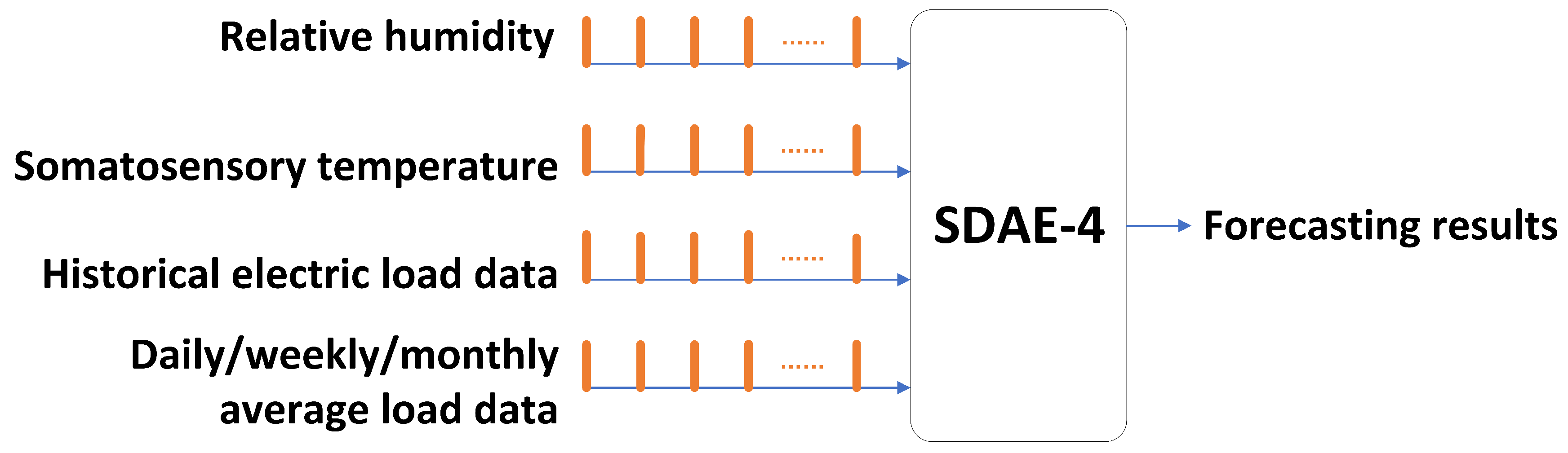
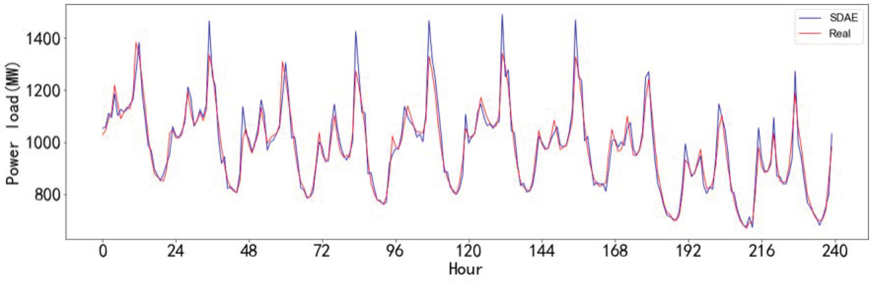
After data pre-processing, the historical load, the somatosensory temperature, the relative humidity, and the daily average load of the Chinese city Fuyang from January 2013 to September 2013 are selected as the dataset. Figure 7 is the schematic diagram of the framework of SDAE-4. The entire data are divided into the 90% training datasets and the 10% forecasting datasets. In addition, 75% of the training datasets are used to train the model and 25% are used to test the model performance. Finally, SDAE-4 with two hidden layers (1-2-1), BP neural network and AE are chosen in the comparison. All considered algorithms are implemented with Python 3.5. The advantage of SDAE is its capability to continuously update the dataset based on predicted results, which enables it to learn the patterns of previous fluctuations and correct the fluctuation trend of data in the training set by the latter consequence [34]. To clearly exhibit the fitting effect of the model, a part of the fitting result of SDAE-based model in testing datasets is partly shown in Figure 8:
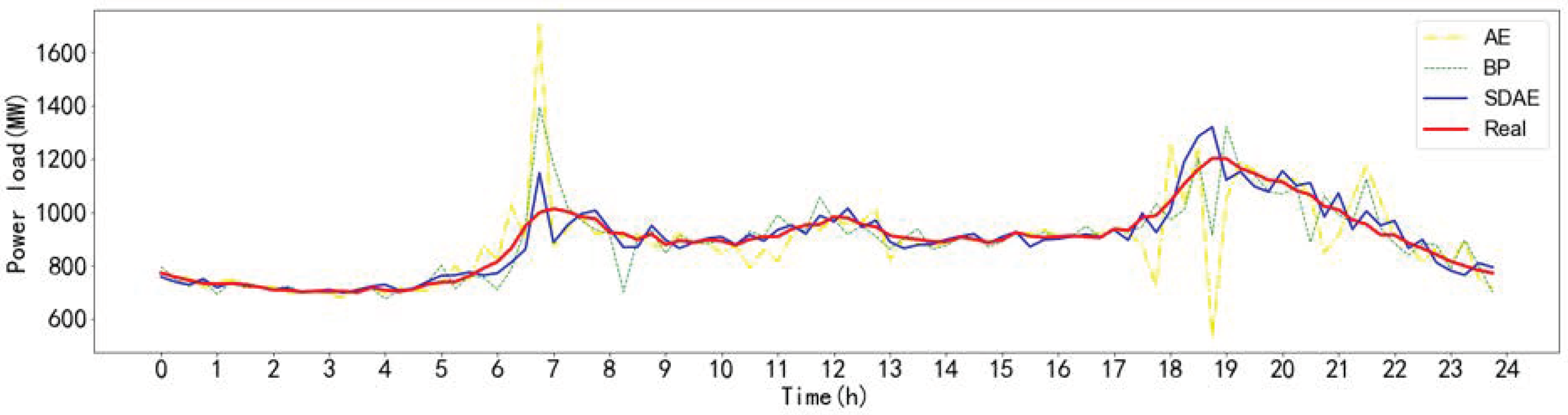
Table 2 compares the average error and maximum error of SDAE-based model from Monday to Sunday and shows that the SDAE-based model can find the periodic change law of historical data. Compared with other days, Saturday’s max MAPE is the biggest probably because Saturday is the transition of weekends and workdays. Figure 9 and Table 3 show the forecast tracking and error comparison of each method.
According to the MAPE, MSE, MAE, RMSE, it can be concluded that the SDAE outperforms other models in electric load forecasting. All of the calculation results prove that the performance of SDAE is better than that of the traditional data driven models when predicting the electric load of the second day. Figure 9 showed that the best forecasting performance is obtained by SDAE. The MAPE of the proposed model is 2.88%. Overall, the proposed model forecasting values fit the actual values. Additionally, at 7:00 p.m., the forecasting value of the proposed model is also closer to the actual value than other algorithms. From 6:00 p.m. to 7:00 p.m., only the proposed model accurately forecasts the changing trend of actual load values. The forecasting trends of other models are opposite to the actual trend. Such opposite forecasting will lead to undesirable outcomes if it occurs in the real condition.
5. Conclusions and Future Work
In this paper, the proposed method is validated by the actual data of the Chinese city Fuyang and the performance of the proposed method is evaluated by comparing the prediction results of the SDAE-based model with other algorithms.
In order to reflect the periodicity of historical data in the dataset, this paper selects the daily average load as the fourth factor and uses it as the baseline. Experiments show that this model can find the periodicity based on this factor. The results also reveal that the unsupervised learning approach using the SDAE model is feasible in load forecasting, and, because it only uses four dimensions in the dataset, it can reduce the computational complexity of the model.
In the load forecasting task of the deep network, since the SDAE neural network uses the idea of the greedy algorithm to pre-train and fine-tune layer by layer, the problems of over-fitting and gradient vanishing are solved in our research. The proposed method is expected to be a key technique for demand side management, energy storage system scheduling, and energy trading platforms in future smart grids.
In future work, the sample size will be expanded to examine the forecasting performance of the model when seasonal factors are considered. In addition, the SDAE-based model will be combined with other neural networks such as LSTM and GRU in the search for better forecasting performance.
Author Contributions
Conceptualization, P.L., P.Z.; Methodology, P.L., P.Z.; Software, P.Z. and Z.C.; Validation, P.L. P.Z. and Z.C.; Writing—original draft, P.Z. and Z.C.; Writing—review & editing, P.Z. and Z.C.
Funding
This research was funded by National Key R&D Program of China(No.2017YFC0804800).
Conflicts of Interest
The authors declare no conflict of interest.
References
- Lai, C.S.; Tao, Y.; Xu, F.; Ng, W.W.; Jia, Y.; Yuan, H.; Huang, C.; Lai, L.L.; Xu, Z.; Locatelli, G. A robust correlation analysis framework for imbalanced and dichotomous data with uncertainty. Inform. Sci. 2019, 470, 58–77. [Google Scholar] [CrossRef]
- Hernandez, L.; Baladron, C.; Aguiar, J.M.; Carro, B.; Sanchez-Esguevillas, A.J.; Lloret, J.; Massana, J. A Survey on Electric Power Demand Forecasting: Future Trends in Smart Grids, Microgrids and Smart Buildings. IEEE Commun. Surv. Tutor. 2014, 16, 1460–1495. [Google Scholar] [CrossRef]
- Xiu-lan, S.; De-feng, H.; Li, Y. Bilinear models-based short-term load rolling forecasting of smart grid. In Proceedings of the 31st Chinese Control Conference, Hefei, China, 25–27 July 2012; pp. 6826–6829. [Google Scholar]
- Amral, N.; Ozveren, C.S.; King, D. Short term load forecasting using Multiple Linear Regression. In Proceedings of the 2007 42nd International Universities Power Engineering Conference, Brighton, UK, 4–6 September 2007; pp. 1192–1198. [Google Scholar]
- Lee, C.M.; Ko, C.N. Short-term load forecasting using lifting scheme and ARIMA models. Expert Syst. Appl. 2011, 5, 5902–5911. [Google Scholar] [CrossRef]
- Taylor, J.W. Short-Term Load Forecasting With Exponentially Weighted Methods. IEEE Trans. Power Syst. 2012, 2, 458–464. [Google Scholar] [CrossRef]
- Huang, N.; Lu, G.; Xu, D. A Permutation Importance–Based Feature Selection Method for Short-Term Electricity Load Forecasting Using Random Forest. Energies 2016, 9, 767. [Google Scholar] [CrossRef]
- Moon, J.; Kim, Y.; Son, M.; Hwang, E. Hybrid Short-Term Load Forecasting Scheme Using Random Forest and Multilayer Perceptron. Energies 2018, 11, 3283. [Google Scholar] [CrossRef]
- Ceperic, E.; Ceperic, V.; Baric, A. A Strategy for Short-Term Load Forecasting by Support Vector Regression Machines. IEEE Trans. Power Syst. 2013, 11, 4356–4364. [Google Scholar] [CrossRef]
- Merkel, G.; Povinelli, R.; Brown, R. Short-Term Load Forecasting of Natural Gas with Deep Neural Network Regression. Energies 2018, 11, 2018. [Google Scholar] [CrossRef]
- Hossen, T.; Plathottam, S.J.; Angamuthu, R.K.; Ranganathan, P.; Salehfar, H. Short-term load forecasting using deep neural networks (DNN). In Proceedings of the 2017 North American Power Symposium (NAPS), Morgantown, WV, USA, 17–19 September 2017; pp. 1–6. [Google Scholar]
- Goodfellow, I.; Bengio, Y.; Courville, L. Deep Learning; MIT Press: Cambridge, UK, 2016; Volume 1. [Google Scholar]
- Chen, X.; Liu, X.; Wang, Y.; Gales, M.J.F.; Woodland, P.C. Efficient Training and Evaluation of Recurrent Neural Network Language Models for Automatic Speech Recognition. IEEE/ACM Trans. Audio Speech Lang. Process. 2016, 11, 2146–2157. [Google Scholar] [CrossRef]
- Li, X.; Wu, X. Constructing long short-term memory based deep recurrent neural networks for large vocabulary speech recognition. In Proceedings of the 2015 IEEE International Conference on Acoustics, Speech and Signal Processing (ICASSP), Brisbane, QLD, Australia, 2015; pp. 4520–4524. [Google Scholar]
- Mayer, H.; Gomez, F.; Wierstra, D.; Nagy, I.; Knoll, A.; Schmidhuber, J. A System for Robotic Heart Surgery that Learns to Tie Knots Using Recurrent Neural Networks. In Proceedings of the 2006 IEEE/RSJ International Conference on Intelligent Robots and Systems, Beijing, China, 9–15 October 2006; pp. 543–548. [Google Scholar]
- Sundermeyer, M.; Ney, H.; Schlüter, R. From Feedforward to Recurrent LSTM Neural Networks for Language Modeling. IEEE/ACM Trans. Audio Speech Lang. Process. 2015, 3, 517–529. [Google Scholar] [CrossRef]
- Senjyu, T.; Mandal, P.; Uezato, K.; Funabashi, T. Next, day load curve forecasting using recurrent neural network structure. IEE Proc. Gen. Trans. Distrib. 2004, 5, 388–394. [Google Scholar] [CrossRef]
- Shi, H.; Xu, M.; Li, R. The title of the cited articleDeep Learning for Household Load Forecasting—A Novel Pooling Deep RNN. IEEE Trans. Smart Grid 2018, 9, 5271–5280. [Google Scholar] [CrossRef]
- Hochreiter, S.; Schmidhuber, J. Long Short-Term Memory. Neural Comput. 1997, 9, 1735–1780. [Google Scholar] [CrossRef] [PubMed]
- Kong, W.; Dong, Z.Y.; Jia, Y.; Hill, D.J.; Xu, Y.; Zhang, Y. Short-Term Residential Load Forecasting Based on LSTM Recurrent Neural Network. IEEE Trans. Smart Grid 2019, 1, 841–851. [Google Scholar] [CrossRef]
- Tian, C.; Ma, J.; Zhang, C.; Zhan, P. A Deep Neural Network Model for Short-Term Load Forecast Based on Long Short-Term Memory Network and Convolutional Neural Network. Energies 2018, 12, 3493. [Google Scholar] [CrossRef]
- Kim, M.; Choi, W.; Jeon, Y.; Liu, L. A Hybrid Neural Network Model for Power Demand Forecasting. Energies 2019, 12, 931. [Google Scholar] [CrossRef]
- Gan, D.; Wang, Y.; Zhang, N.; Zhu, W. Enhancing short-term probabilistic residential load forecasting with quantile long–short-term memory. J. Eng. 2017, 2017, 2622–2627. [Google Scholar] [CrossRef]
- Bouktif, S.; Fiaz, A.; Ouni, A.; Serhani, M.A. Single and Multi–Sequence Deep Learning Models for Short and Medium Term Electric Load Forecasting. Energies 2019, 12, 149. [Google Scholar] [CrossRef]
- Cho, K.; Van Merriënboer, B.; Gulcehre, C.; Bahdanau, D.; Bougares, F.; Schwenk, H.; Bengio, Y. Learning Phrase Representations using RNN Encoder–Decoder for Statistical Machine Translation. arXiv 2014, arXiv:1406.1078. [Google Scholar]
- Wang, Y.; Liao, W.; Chang, Y. Gated Recurrent Unit Network–Based Short-Term Photovoltaic Forecasting. Energies 2018, 11, 2163. [Google Scholar] [CrossRef]
- Vincent, P.; Larochelle, H.; Lajoie, I.; Bengio, Y.; Manzagol, P.A. Stacked denoising auotoencoders: Learning useful representations in a deep network with a local denoising criterion. Mach. Learn. Res. 2010, 11, 3371–3408. [Google Scholar]
- Hinton, G.E.; Salakhutdinov, R.R. Reducing the dimensionality of data with neural network. Science 2006, 7, 504–507. [Google Scholar] [CrossRef]
- Ye, X.; Wang, L.; Xing, H.; Huang, L. Denoising hybrid noises in image with stacked autoencoder. In Proceedings of the IEEE International Conference on Information and Automation, Lijiang, China, 8–10 August 2015; pp. 2720–2724. [Google Scholar]
- Gu, F.; Khoshelham, K.; Valaee, S.; Shang, J.; Zhang, R. Locomotion Activity Recognition Using Stacked Denoising Autoencoders. IEEE Internet Things J. 2018, 6, 2085–2093. [Google Scholar] [CrossRef]
- Du, B.; Xiong, W.; Wu, J.; Zhang, L.; Zhang, L.; Tao, D. Stacked Convolutional Denoising Auto-Encoders for Feature Representation. IEEE Trans. Cybernet. 2017, 4, 1017–1027. [Google Scholar] [CrossRef]
- Vincent, P.; Larochelle, H.; Bengio, Y.; Manzagol, P.A. Extracting and Composing Robust Features with Denoising Auto conder. In Proceedings of the 25th International Conference on Machine Learning, Helsinki, Finland, 5–9 July 2008; Volume 10, pp. 1096–1103. [Google Scholar]
- Rostami, T. Adaptive color mapping for NAO robusting neural network. Adv. Comput. Sci. Int. J. 2015, 3. [Google Scholar]
- Kuo, J.Y.; Pan, C.W.; Lei, B. Using Stacked Denoising Autoencoder for the Student Dropout Prediction. In Proceedings of the 2017 IEEE International Symposium on Multimedia (ISM), Taichung, Taiwan, 11–13 December 2017; pp. 483–488. [Google Scholar]
- LeCun, Y.; Bengio, Y.; Hinton, G. Deep learning. Nature 2015, 521, 436–444. [Google Scholar] [CrossRef]
- Liang, J.; Liu, R. Stacked Denoising Autoencoder and Dropout Together to Prevent Overfitting in Deep Neural Network. In Proceedings of the 2015 8th International Congress on Image and Signal Processing (CISP), Shenyang, China, 14–16 October 2015; Volume 10, pp. 697–701. [Google Scholar]
- Glorot, X.; Bengio, Y. Understanding the difficulty of training deep feedforward neural networks. In Proceedings of the Thirteenth International Conference on Artificial Intelligence and Statistics, Sardinia, Italy, 13–15 May 2010; pp. 249–256. [Google Scholar]
- Wang, L.; Zhang, Z.; Chen, J. Short-Term Electricity Price Forecasting With Stacked Denoising Autoencoders. IEEE Trans. Power Syst. 2017, 7, 2673–2681. [Google Scholar] [CrossRef]
- Historical Weather Data of Fuyang. Available online: https://tianqi.911cha.com (accessed on 1 March 2019).
Figure 1.
Schematic diagram of auto-encoder (AE).

Figure 2.
Schematic diagram of denoising auto-encoder (DAE).

Figure 3.
Schematic diagram of double denoising auto-encoder.

Figure 4.
Schematic diagram of stacked denoising auto-encoder (SDAE).

Figure 5.
Schematic diagram of the whole algorithm with the SDAE Model.

Figure 6.
The framework of SDAE-13.

Figure 7.
The framework of SDAE-4.

Figure 8.
Fitting results of the SDAE-based model.

Figure 9.
The comparisons of load forecasting results for a certain day.


Table 1.
The comparison of average load prediction.
| Metric | DA | WA | MA |
|---|---|---|---|
| MSE/MW | 316.93 | 19,066.71 | 25,043.12 |
| MAE/MW | 14.56 | 119.54 | 158.25 |
| RMSE/MW | 10.41 | 79.80 | 158.25 |
Table 2.
The comparison of errors for Monday to Sunday.
| Week | Average MAPE | Max MAPE | Average MSE/MW | Max MSE/MW |
|---|---|---|---|---|
| Monday | 2.87% | 13.05% | 1470.09 | 20,208.65 |
| Tuesday | 2.84% | 14.89% | 1474.40 | 22,878.74 |
| Wednesday | 2.94% | 13.51% | 1509.40 | 24,338.06 |
| Thursday | 2.90% | 14.00% | 1547.41 | 22,898.14 |
| Friday | 2.88% | 13.57% | 1506.83 | 20,218.29 |
| Saturday | 2.85% | 15.89% | 1580.70 | 28,186.05 |
| Sunday | 2.82% | 13.66% | 1592.79 | 26,784.63 |
Table 3.
Comparison of errors of different forecasting methods.
| MAPE | MSE/WM | MAE/WM | RMSE/WM | |
|---|---|---|---|---|
| SDAE | 2.88% | 1524.44 | 27.99 | 27.22 |
| BP | 3.66% | 4030.83 | 35.19 | 56.51 |
| AE | 6.16% | 12,082.66 | 56.61 | 94.24 |
© 2019 by the authors. Licensee MDPI, Basel, Switzerland. This article is an open access article distributed under the terms and conditions of the Creative Commons Attribution (CC BY) license (http://creativecommons.org/licenses/by/4.0/).
Share and Cite
MDPI and ACS Style
Liu, P.; Zheng, P.; Chen, Z. Deep Learning with Stacked Denoising Auto-Encoder for Short-Term Electric Load Forecasting. Energies 2019, 12, 2445. https://doi.org/10.3390/en12122445
AMA Style
Liu P, Zheng P, Chen Z. Deep Learning with Stacked Denoising Auto-Encoder for Short-Term Electric Load Forecasting. Energies. 2019; 12(12):2445. https://doi.org/10.3390/en12122445
Chicago/Turabian StyleLiu, Peng, Peijun Zheng, and Ziyu Chen. 2019. "Deep Learning with Stacked Denoising Auto-Encoder for Short-Term Electric Load Forecasting" Energies 12, no. 12: 2445. https://doi.org/10.3390/en12122445
Note that from the first issue of 2016, this journal uses article numbers instead of page numbers. See further details here.