A Unified and Efficient Approach to Power Flow Analysis

Abstract

Highly nonlinear and nonconvex power flow analysis plays a key role in the monitoring, control, and operation of power systems. There is no analytic solution to power flow problems, and therefore, finding a numerical solution is oftentimes an aim of modern computation in power system analysis. An iterative Newton-Raphson method is widely in use. While most times this method finds a solution in a reasonable time, it often involves numerical robustness issues, such as a limited convergence region and an ill-conditioned system. Sometimes, the truncation error may not be small enough to ignore, which can make the iterative process significantly expansive. We propose a new unified framework, based on the Kronecker product, that does not involve any truncation, and which is bilinear to make it possible to incorporate statistical analysis. The proposed method is tested for power flow, state estimation, probabilistic power flow, and optimal power flow studies on various IEEE model systems.

1. Introduction

Power flow analysis focuses on power systems in normal steady-state operation, as well as transient stability, static voltage stability, and contingency studies. It is important for determining dispatch, and in monitoring systems in terms of state estimation. It aims to find the complex voltage at each bus, and the complex power flows at the ends of each line at the steady-state operating conditions, in order to satisfy the Kirchhoff’s laws [1] that specify apparent power as $v_j{I}_j^{*}=v_j{\left(e_j^T{Y}_{bus}v\right)}^{*}$. The use of the power flow algorithm is extended to the state estimator, to provide the information necessary to execute security analysis. In modern power system operation, various sources of uncertainty are integrated, such as renewables and demand control [2,3]. For a reliable operation, the range of state variables needs to be determined by mapping the uncertain injection through power flow methods. Probabilistic power flow problems [4,5,6,7,8] estimate the system performance over wide range of the dispatches. An interested reader may find [7] to be a useful review. Optimal power flow (OPF), a power system operation tool introduced by Carpentier [9], is a highly nonconvex, and nonlinear problem. Many approaches have been pursued to solve the nonlinear and nonconvex nature of a full OPF problem [10,11,12,13]. However, the curse of dimensionality and the nonconvex nature of the problem make it impossible for an algorithm to guarantee a convergence, and therefore, only heuristic approaches have focused on finding a numerical solution [14,15]. Recently, various attempts have been made to identify a solution, including the use of stochastic and probabilistic methods [16], such as simulated annealing [17], direct Monte-Carlo sampling [18], mean field theory [19], and deterministic methods, including a cutting plane [20], branch and bound (B&B) [21], and branch and cut [22]. To address the nonconvex nature of OPF, Bai [23] introduced the conversion of the OPF problem into semi-definite programming (SDP). Thereafter, Lavaei and Low [24] showed that the solution of SDP-OPF could be the global optimizer of the original OPF problem in the form of nonlinear programming, if—and only if—the solution satisfies a rank requirement. Lesieutre and Molzahn [25] later presented a case showing that the solution in [25] did not satisfy the rank requirement. Josz et al. [26] modified rank relaxation and found the rank-satisfied solutions. However, this method cannot handle cases larger than the five-bus system because of high runtime costs. For power system monitoring, the state estimator aims to estimate the voltages that match with the sensor measurements, typically SCADA (supervisory control and data acquisition) and PMU (phasor measurement units). The measurement errors come from the synchronous measurement errors in voltages, current, and flows, as well as from the data transfer and from asynchronous measurements. Therefore, the performance of the state estimator may suffer from the linear approximation of Taylor series expansion to apply the Newton-Raphson approach.

For a mesh power system with more than two buses, no analytic solution is found, and the research activities have been focused on finding a numerical solution. While a non-iterative approach such as holomorphic embedding [27] is possible, iterative approaches are usually pursued for their computational efficiency, including the Newton–Raphson method, Gauss-Seidel method, and the decoupled power flow method [1]. Recently, other heuristic approaches, like the genetic algorithm [28] and particle swam optimization approach [29], are taken into consideration, but they also execute Newton-Raphson updates in their inner loop. A typical disadvantage of the Newton-Raphson method is the computational cost for factorizing and updating the Jacobian matrix during the iterative solution process. The approach that the Newton-Raphson method takes is summarized as follows: at a given point, one takes the Taylor series expansion of a nonlinear function; ignore second or higher-order terms so as to construct a linear iteration equation AΔx + b = 0; the next step is computed by solving the linear equation for Δx. The advancement in modern computation, especially the efficient methods of utilizing the structure of the Jacobian A, such as symmetry and sparsity, reduces this computation cost significantly; as a result, the Newton-Raphson method is widely used in power flow analysis. Even though the heuristic approaches based on the Newton-Raphson method finds a numerical solution with a reasonable computation cost, there are several computational issues, including numerical robustness and strong initial point dependence [1], either when A is ill-conditioned at the iteration or when the second or higher order terms can be too large to ignore.

This paper is organized as follows. Section 2 introduces a unified framework for power flow analysis. Section 3 presents a solution algorithm and the proof for the convergence. Section 4 shows the results and discussions, and Section 5 presents conclusions. In this paper, for improving the readability, variables are italicized, vectors are in the lower case and in boldface, and matrices are in the upper case and in boldface. All the complex vectors are partitioned in a way that all the real components are listed first, and then all the imaginary components follow.

2. United Framework

Even though power flow analysis is a backbone of power flow, optimal power flow, probabilistic power flow, and state estimation, each problem has its own problem formulation. For example, f(v) = 0 for power flow problems; for the minimization for optimal power flow problems; for minimizing the mismatch while satisfying power balance equations over uncertain power generation, as well as demand for probabilistic power flow problems; and for the weighted least square in the discrepancy between measurements and the estimates for the state estimation, etc. In Section 2, we propose a unified framework to incorporate the problems and new solution method outlined in Section 3, to solve the problem using the Kronecker product. The proposed algorithm is robust in terms of numerical computation, and a local convergence is proven.

2.1. Power Flow Problems

To unequivocally define the state of a system, one should have the values for the voltages and the injections at each bus (4N variables). Since one voltage angle is set to a fixed number at a voltage reference bus (zero in general), there are 4N-1 variables. For solving a set of nonlinear equations with 4N-1 variables, the necessary condition (not-sufficient condition) is to have 4N-1 independent equations. At each bus, while two voltages and two power injections are unknowns, two power balance equations (Kirchhoff’s laws) are provided, not including the slack bus, i.e., the 2N-1 equations. Therefore, we need to assign 2N variables for the system. Even though it is not necessary to assign two variables at each bus, we conventionally do. For example, we assign power injections at PQ buses, voltage magnitude and real power injection at PV buses, and voltages at the slack bus. This conventional approach is based upon the characteristics of the components that are directly connected to a bus. However, as renewables are integrated into the grid systems, the definition of a bus with a renewable generator is questionable. It can be a PV bus, since it is directly connected to a generator, but it may experience difficulty in controlling voltage magnitudes. For some buses, it would be important to control the reactive power injection for reliable system operation. Then the bus can be QV bus. Therefore, in this study, we suggest that 2N variables over the system be assigned regardless of the location. For an extreme case, we may assign two voltages and two injections at some buses, while none is assigned for other buses. Power injections or voltage magnitude squares are as follows (see the detailed derivation in Appendix A):

$${\left[vec\left(M_j\right)\right]}^T\left(x_{PF}\otimes x_{PF}\right)-{\xi }_j=0,j=1,\cdots ,2N-1$$

(1)

where M and ξ are the matrix and the right-hand side, respectively regarding either the power injection or the square of voltage magnitudes; and x_PF = v. To prevent (1) from being an overdetermined system, only 2N-1 equalities are imposed (one slack bus to compensate for the system-wide power balance). For a case with distributed slack buses, 2N equalities are imposed, which results in a distributed mismatch over the network. If there exists a solution to (1), the solution v is also a solution to the following optimization problem, where

$$x_{PF}^{sol}=\underset{x_{PF}}{\arg \min }{\Vert \underset{A_{PF}}{\underbrace{\left[\begin{array}{c}vec{\left(M_1\right)}^T\\ ⋮\\ vec{\left(M_{2N-1}\right)}^T\end{array}\right]}}\left(x_{PF}\otimes x_{PF}\right)-\underset{b_{PF}}{\underbrace{\left(\begin{array}{c}{\xi }_1\\ ⋮\\ {\xi }_{2N-1}\end{array}\right)}}\Vert }_2=\underset{x_{PF}}{\arg \min }{\Vert A_{PF}\left(x_{PF}\otimes x_{PF}\right)-b_{PF}\Vert }_2$$

(2)

A solution to (2) is also a solution to (1) if ${\Vert A_{PF}\left(x_{PF}^{sol}\otimes x_{PF}^{sol}\right)-b_{PF}\Vert }_2$ is 0. Therefore, (1) and (2) are equivalent.

2.2. Optimal Power Flow Problems

OPF is a nonlinear and nonconvex problem, as follows:

$$\underset{\left|v\right|,\theta ,g}{\min }{f}_{OPF}\left(g\right)\mathrm{s}.\mathrm{t}.\{\begin{array}{l}{g}_{eq}\left(\left|v\right|,\theta ,g\right)=0\\ h_{in}\left(\left|v\right|,\theta ,g\right)\le 0\end{array}$$

(3)

$$\underset{x_{OPF}}{\min }{f}_{OPF}\left(x_{OPF}\right)$$

(4)

$$\mathrm{s}.\mathrm{t}.\{\begin{array}{l}{\left[vec\left(M_{eq}^i\right)\right]}^T\left(x_{OPF}\otimes x_{OPF}\right)-{\xi }_{eq}^i=0i=1,\cdots ,2N+4L\\ {\left[vec\left(M_{in}^j\right)\right]}^T\left(x_{OPF}\otimes x_{OPF}\right)-{\xi }_{in}^j=0j=1,\cdots ,2N+2L+2G\end{array}$$

and

$$x_{OPF}={\left(v^T{g}^T{f}^T{z}_f^T{z}_g^T{z}_{\max }^T{z}_{\min }^T{\rho }^T{\mu }_f^T{\mu }_g^T{\mu }_{\max }^T{\mu }_{\min }^{T}1\right)}^T$$

(5)

where, Equations (3) and (4) are the same problem, constructed on the polar coordinate system (Equation (3)) and on the Cartesian coordinate system (Equation (4)). This problem is an NP (nondeterministic polynomial time) complete problem. Many heuristic approaches aim to find a local solution to satisfy the Karush-Kuhn-Tucker (KKT) conditions [30] for Equation (3). Therefore, the working problem for solving Equation (4) becomes:

$$x_{OPF}^T{M}_{\kappa }{x}_{OPF}-{\xi }_{\kappa }=0\leftrightarrow {\left[vec\left(M_{\kappa }\right)\right]}^T\left(x_{OPF}\otimes x_{OPF}\right)-{\xi }_{\kappa }=0$$

(6)

The KKT condition described in (4) is integrated into a bilinear least square problem [31]:

$$\underset{x_{OPF}}{\min }{\Vert \underset{A_{OPF}}{\underbrace{\left[\begin{array}{c}{\left[vec\left(M_1\right)\right]}^T\\ ⋮\\ {\left[vec\left(M_{N_{KKT}}\right)\right]}^T\end{array}\right]}}\left(x_{OPF}\otimes x_{OPF}\right)-\underset{b_{OPF}}{\underbrace{\left(\begin{array}{c}{\xi }_1\\ ⋮\\ {\xi }_{N_{KKT}}\end{array}\right)}}\Vert }_2={\Vert A_{OPF}\left(x_{OPF}\otimes x_{OPF}\right)-b_{OPF}\Vert }_2$$

(7)

where N_KKT is the number of the KKT conditions. A detailed derivation of (3)–(6) is listed in Appendix B.

2.3. Probabilistic Power Flow Problems

The probability of power generation and power demand is generally continuous, and therefore the purpose of probabilistic power flow problems is to determine the voltages that minimize the mismatches between uncertain power injections and planned injections. In probabilistic power flow studies, three approaches are most widely referenced—the analytical method, point estimation, and the numerical approach. Analytical methods aim to get cumulants of output from cumulants of input, based upon a linear approximation of AC power flow [8]. Although the approach is efficient for a large-scale system, due to its reduced computation costs, the precision critically depends upon an operation point chosen for the linearization. The other two approaches preserve the nonlinearity to some extent. They start with modeling the stochastic nature of the problem as a deterministic optimization problem with finitely many scenarios. Therefore, the computation efficiency may be low on large-scale power systems. Monte Carlo simulation makes it possible to reduce the number of scenarios to a manageable size. The sample average approximation gives a reasonably accurate approximation of the true problem. For a fixed y $\in$ Y and an independent identical distribution sample, the sample average converges to the corresponding expectation, at a rate of $\vartheta \left(N^{-0.5}\right)$. Therefore, in order to achieve a reliable result, Monte Carlo simulation methods can be very slow. Su suggested a point-estimate method based on a 2m + 1 approach [32]. The shortcoming of this approach is that it does not reflect the probability distribution, and therefore, the solution to the problem is not a good approximation of the original problem. We propose a following optimization problem to minimize the weighted mismatch, where the weight w reflects the probability distribution. Similar to the power flow studies, the mismatches are either power injection or voltage magnitudes at bus j:

$$\underset{A_j}{\underbrace{\left[\begin{array}{c}{\left[w_{1}vec\left(M_j\right)\right]}^T\\ ⋮\\ {\left[w_{N_{scenario}^j}vec\left(M_j\right)\right]}^T\end{array}\right]}}\left(x_{PPF}\otimes x_{PPF}\right)-\underset{b_j}{\underbrace{\left(\begin{array}{c}{w}_1{\xi }_j\\ ⋮\\ w_{N_{scenario}^j}{\xi }_{N_{scenario}^j}\end{array}\right)}}=0\to A_j\left(x_{PPF}\otimes x_{PPF}\right)-b_j=0$$

(8)

where x_PPF is voltage for this problem (x_PPF = v), and $N_{scenario}^j$ is the number of scenarios at bus j. Note that there can exist multiple power balance equations or nodal voltage magnitudes at the same bus with multiple probabilities. For example, at bus 1—the only one wind turbine is connected to—wind output is 70 MW with a probability of 25%, and 20 MW with a probability of 75%. Then (8) in per unit basis of 100 MW base MVA includes; $w_{25\%}\left\{{\left[vec\left(M_1\right)\right]}^T\left(x_{PPF}\otimes x_{PPF}\right)-0.7\right\}=0$ and $w_{75\%}\left\{{\left[vec\left(M_1\right)\right]}^T\left(x_{PPF}\otimes x_{PPF}\right)-0.2\right\}=0$. Therefore, Equation (8) can be an overdetermined system, and the solution x_PPF may not result in a zero mismatch when all possible scenarios are taken into consideration. The advantage of Equation (8) is that the variable x_PPF = v is clearly separated from inputs (data matrix and weight factor associated with probability).

2.4. State Estimation Problems

State estimation plays a central role in monitoring for reliable control power systems. Power flows and voltage magnitudes are measured through asynchronous SCADA (supervisory control and data acquisition) systems every 2–3 seconds. PMUs (phasor measurement units) are integrated to enhance the real-time situational awareness under the smart grid umbrella. PMUs provide synchronized direct measure of the voltages at 60 Hz. Significant studies have focused on the integration of PMU data in the power system state estimator. To combine two sets of data, two approaches are most widely used: (1) direct use of a PMU to get the voltages at observable buses, and then estimate them at the other buses; and (2) incorporating the SCADA and PMU simultaneously [33,34]. For the first method, inadequate estimate of voltages from PMUs using SCADA affects the performance.

All the methods descried above perform the traditional state estimation with SCADA and PMU when both signals are available:

$$\frac{\partial }{\partial v}{\Vert u-fun\left(v\right)\Vert }_2^2=\frac{\partial }{\partial v}{\Vert \left(u-fun\left(v_0\right)\right)-A\left(v-v_0\right)-\vartheta \left({\Vert v\Vert }_2^2\right)\Vert }_2^2=0\to v=v_0+{\left(A^{T}A\right)}^{-1}{A}^T\left(u-fun\left(v_0\right)\right)$$

(9)

where u is the measurement, either from SCADA or from PMU sensors. Equation (9) yields the updated voltages from v₀. The process in Equation (9) is repeated until the mismatch is small enough. Equation (9) is an efficient approach for conventional state estimation with SCADA, but only when the measurements are all in quadratic to voltages. When PMU measurements are combined so that they linear to voltages, the truncation error lies in SCADA only. Therefore, Equation (9) may not be able to estimate a proper state, and it is desirable not to truncate higher order terms. Suppose u_PMU and u_SCADA are measurements from PMU and SCADA, respectively. Equation (10) is formulated to minimize the measurement errors:

$$\underset{v}{\min }{\Vert {\epsilon }_{SE}\Vert }_2^2=\underset{v}{\min }{\Vert A_{SE}\left(x_{SE}\otimes x_{SE}\right)-b_{SE}\Vert }_2^2$$

(10)

where ε_SE, A_SE, and b_SE are the weighted mismatch vector, weighted matrices associated with measurements, and measurements, respectively; and x_SE = [v^T 1]^T. A detailed derivation is listed in Appendix C.

2.5. Summary

A unified model for power flow analysis—power flow, optimal power flow, probabilistic power flow, and state estimation—is proposed. In the model, power flow analysis to identify a solution x^sol is shown in Equation (11):

$$x^{sol}=\underset{x}{\arg \min }{\Vert A\left(x\otimes x\right)-b\Vert }_2$$

(11)

Note that A is sparse, since the matrices associated with A are originally sparse, and vectorization of the matrices does not alter the sparsity.

3. Solution Algorithm

3.1. Alternating Least Square Approach

Equation (11) can be further simplified with a property of the Kronecker product, $\left(A\otimes B\right)\left(C\otimes D\right)=\left(AC\right)\otimes \left(BD\right)$:

$$b-A\left(x\otimes x\right)\leftrightarrow \{\begin{array}{l}b-\left[A\left(x\otimes I\right)\right]x\\ b-\left[A\left(I\otimes x\right)\right]x\end{array}$$

(12)

Equation (12) is the recipe to apply an alternating least square (ALS) algorithm to solve (11).

$$\begin{array}{l}StepI:\underset{x}{\min }\Vert b-\left[A\left(x_l\otimes I\right)\right]x\Vert \to {\widehat{x}}_l\left(={\left[A\left(x_l\otimes I\right)\right]}^{-1}b\right)\\ StepII:\underset{x}{\min }\Vert b-\left[A\left(I\otimes {\widehat{x}}_l\right)\right]x\Vert \to {\widehat{x}}_{l+1}\left(={\left[A\left(I\otimes {\widehat{x}}_l\right)\right]}^{-1}b\right)\\ StepIII:x_{l+1}=\left(1-\alpha \right){\widehat{x}}_l+\alpha {\widehat{x}}_{l+1},0<\alpha \le 0.5\end{array}$$

(13)

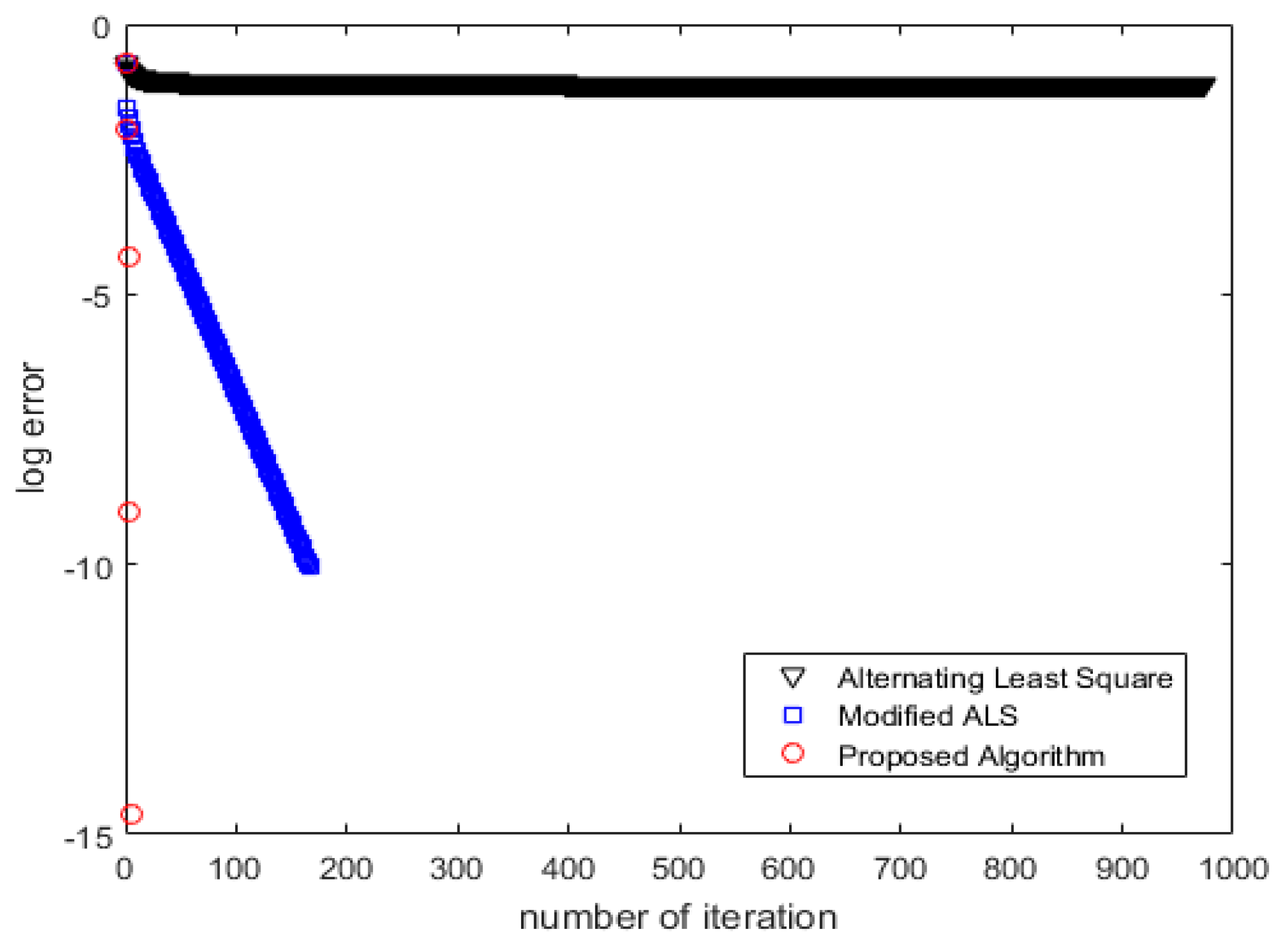
As noted before, A is sparse. Even though x is a dense vector, the Kronecker products with an identity matrix—$x_l\otimes I$ and $I\otimes {\widehat{x}}_l$—are sparse. The inner products $A\left(x_l\otimes I\right)$ and $A\left(I\otimes {\widehat{x}}_l\right)$ are also sparse, which makes the numerical computations in Equation (13) efficient. Step III is imposed to ensure consistency between the right and the left variable x. This simple step makes the computation highly efficient. However, it is not possible to prove the convergence of this modified ALS. The left and the right variable x should be consistent; however, the conventional ALS algorithm does not guarantee the consistency. Therefore, the conventional ALS algorithm converges a suboptimal solution. The modified ALS algorithm finds the solution regardless of choice of α (α = 0.5 for the results shown in Figure 1).

Even if the modified ALS finds the solution, it takes approximately 200 iterations. Multiple initial points were tested to see if they result in a different solution; however, they all returned the same numerical solution. As shown in Figure 1, it is clear that the proposed algorithm presented in Section 3.2 outperforms the conventional ALS algorithm in terms of finding a proper solution and computational efficiency, both in the quality of the solution and the lower number of iterations to get to the solution. Therefore, the proposed Kronecker least-square approach is most suitable for precise computation. The computation times of ALS, modified ALS, and the proposed method are approximately 1000, 200, and 1 second, respectively. All computations were performed with a Dell Precision M6700 (CPU: Intel Core i7-3840QM CPU @ 2.80 GHz).

3.2. Newton-Raphson Method

The Newton-Raphson method is most widely used for solving nonlinear equations. It numerically finds the next step by taking a Taylor Series expansion at the current step, and truncating quadratic and higher-order terms. For example, with N_tot equations,

$$\Delta x_{l+1}={\mathsf{\Omega }}^{-T}\left[b-A\left(x_l\otimes x_l\right)\right]\mathrm{where}\mathsf{\Omega }=\left[\left(2A_1{x}_l\right)\cdots \left(2A_{N_{tot}}{x}_l\right)\right]$$

(14)

where Ω is a concatenated matrix, of which the kth column vector is 2A_kx_l. Equation (14) may not be numerically robust when the Jacobian matrix in the square bracket is ill-conditioned. To meet the linear equality and inequality constraints in Equation (3), a partial update is proposed in the MATPOWER Interior Point Solver (MIPS) [15]. The primal and dual variables in x_OPF are updated separately in the study [15]. While it heuristically seldom fails to find a solution, the convergence is not proven for the method with the differentiation of the updating factors.

3.3. Proposed Method

At the lth iteration, let ${\widehat{x}}_{l+1}$ be an optimizer to the following least square problem:

$${\widehat{x}}_{l+1}=\arg \underset{x}{\min }{\Vert b-\frac{1}{2}\left[A\left(I\otimes x_l+x_l\otimes I\right)\right]x\Vert }_{{}_2}$$

(15)

It is advantageous to compute the matrix inside the square bracket in Equation (15), since it is a linear update of a fixed matrix A with x_l, compared to the computation of the Jacobian matrix of the Newton-Raphson method in the polar coordinate system. In our interior-point method, at the lth iteration, we update x to move in the direction toward ${\widehat{x}}_{l+1}$, but only up to the ratio of α_l, $0<{\alpha }_l\le 0.5$.

$$x_{l+1}\leftarrow \left(1-{\alpha }_l\right)x_l+{\alpha }_l{\widehat{x}}_{l+1}\mathrm{OR}{x}_l+{\alpha }_l\left({\widehat{x}}_{l+1}-x_l\right)$$

(16)

Furthermore, we constrain that α_l approaches 0.5 as the number of iterations increases. In the vicinity of the solution, similar to a linear approximation in the Newton–Raphson method, we can assume that the change in x, x_l+1 − x_l, is sufficiently small. For example, where δ is a sufficiently small number, ${\Vert x_{l+1}-x_l\Vert }_2\left(={\alpha }_l{\Vert {\widehat{x}}_{l+1}-x_l\Vert }_2\right)$$\le \sqrt{\delta /{\Vert \tilde{A}\Vert }_2}$. Therefore, the two-norm error in Equation (15) is:

$${\Vert {\epsilon }_{l+1}\Vert }_{{}_2}={\Vert b-A\left[\left(x_l+\Delta x_{l+1}\right)\otimes \left(x_l+\Delta x_{l+1}\right)\right]\Vert }_2\le 2{\alpha }_l{\Vert b-\frac{1}{2}A\left(I\otimes x_l+x_l\otimes I\right){\widehat{x}}_{l+1}\Vert }_2+\left(1-2{\alpha }_l\right){\Vert {\epsilon }_l\Vert }_2$$

(17)

where ${\epsilon }_l=b-A\left(x_l\otimes x_l\right)$. Note that the second term in the bracket equals the half of the Jacobian in the Newton–Raphson method in the Cartesian coordinate system. The two-norm error at (l+1)th iteration in updating x depends on the choice of α_l, as shown in Equation (17). Then, the error at the (l+1)th solution generated by the algorithm is no greater than that at the previous iteration:

$$\begin{array}{cc}\hfill {\Vert {\epsilon }_{l+1}\Vert }_2& \le 2{\alpha }_l{\Vert b-\frac{1}{2}A\left(I\otimes x_l+x_l\otimes I\right){\widehat{x}}_{l+1}\Vert }_2+\left(1-2{\alpha }_l\right){\Vert {\epsilon }_l\Vert }_2\hfill \\ & \le 2{\alpha }_l{\Vert b-\frac{1}{2}A\left(I\otimes x_l+x_l\otimes I\right)x_l\Vert }_2+\left(1-2{\alpha }_l\right){\Vert {\epsilon }_l\Vert }_2={\Vert {\epsilon }_l\Vert }_2\hfill \end{array}$$

(18)

The second inequality holds because ${\widehat{x}}_{l+1}$ is the optimizer of convex problems in Equation (15), where the feasible region includes x_l. The proposed algorithm is outlined as

Algorithm

Set l = 0 (l: iteration index) and εth (tolerance in error)

(1) If $\Vert {\epsilon }_l{\Vert }_2\le {\epsilon }_{th}$, terminate the process;

(2) Otherwise compute ${\widehat{x}}_{l+1}$ using Equation (15);

(3) Update $x_{l+1}\leftarrow x_l+{\alpha }_l\left({\widehat{x}}_{l+1}-x_l\right)$, l ← l+1, go to Equation (1).

3.4. Convergence of the Proposed Method

Suppose $x_{\infty }$ is a root of a Lipschitz continuous function $F\left(x\right)=b-A\left(x\otimes x\right)=0$, and x_l is sufficiently close to $x_{\infty }$. For a vector ${\epsilon }_l$ where ${\epsilon }_l=x_{\infty }-x_l$, we obtain

$$0=F\left(x_{\infty }\right)=F\left(x_l+{\epsilon }_l\right)=b-A\left(x_l+{\epsilon }_l\right)\otimes \left(x_l+{\epsilon }_l\right)=\underset{F\left(x_l\right)}{\underbrace{b-A\left(x_l\otimes x_l\right)}}\underset{J\left(x_l\right)}{\underbrace{-A\left(I\otimes x_l+x_l\otimes I\right)}}{\epsilon }_l-A\left({\epsilon }_l\otimes {\epsilon }_l\right)$$

(19)

Note that Equation (19) does not involve the truncation of higher order terms. From Equation (16), one finds $x_{l+1}=\left(1-{\alpha }_l\right)x_l-2{\alpha }_l{\left[J\left(x_l\right)\right]}^{-1}b$, which leads to:

$$F\left(x_l\right)=\frac{1}{2{\alpha }_l}J\left(x_l\right)\left(x_l-x_{l+1}\right)$$

(20)

Using Equation (20) in Equation (19) yields

$$J\left(x_l\right)\left(\frac{x_l-x_{l+1}}{2{\alpha }_l}+x_{\infty }-x_l\right)-A\left[\left(x_{\infty }-x_l\right)\otimes \left(x_{\infty }-x_l\right)\right]=0$$

Then. by using the triangular inequality,

$${\Vert {\epsilon }_{l+1}\Vert }_2={\Vert \left(1-2{\alpha }_l\right){\epsilon }_l+2{\alpha }_l{\left[J\left(x_l\right)\right]}^{-1}A\left({\epsilon }_l\otimes {\epsilon }_l\right)\Vert }_2\le {\Vert \left(1-2{\alpha }_l\right){\epsilon }_l\Vert }_2+2\left|{\alpha }_l\right|{\Vert {\left[J\left(x_l\right)\right]}^{-1}A\left({\epsilon }_l\otimes {\epsilon }_l\right)\Vert }_2$$

(21)

For a sufficiently large l, α_l becomes 0.5 and the second term is in quadratic. Therefore, the proposed algorithm is super-linear.

We also propose a direct method that ensures α_l is always 0.5, regardless of l. The only difference between our interior-point and direct methods is how to choose α_l. It is observed that because f(x) is a Lipschitz continuous function, the norm of its inverse Jacobian matrix [J(x)]⁻¹ is well-bound. Consequently, using the Cauchy-Schwarz inequality [31], the proposed algorithm’s convergence is quadratic:

$${\Vert {\epsilon }_{l+1}\Vert }_2\le \left(1-2{\alpha }_l\right){\Vert {\epsilon }_l\Vert }_2+2{\alpha }_l{\Vert {\left[J\left(x_l\right)\right]}^{-1}\Vert }_2{\Vert A\Vert }_2{\Vert {\epsilon }_l\otimes {\epsilon }_l\Vert }_2^2={\Vert {\left[J\left(x_l\right)\right]}^{-1}\Vert }_2{\Vert A\Vert }_2{\Vert {\epsilon }_l\Vert }_2^2=\vartheta \left({\Vert {\epsilon }_l\Vert }_2^2\right)$$

(22)

While the Newton-Raphson method relies on the Taylor series expansion and truncation of higher order terms, this proposed algorithm does not involve any approximation, and the error reduces at every iteration, regardless of the choice of an initial guess. Furthermore, it utilizes the numerically stable optimization approach. As a result, the algorithm does not suffer the numerical stability issues of the Newton-Raphson method when the data matrix is ill-conditioned.

3.5. Determination of α_l for the Interior Point Method

The control variable x in OPF problems is comprised of state variables, shadow prices, and slack variables, such as $x_{OPF}={\left(v^T{g}^T{f}^T{z}_f^T{z}_g^T{z}_{\max }^T{z}_{\min }^T{\rho }^T{\mu }_f^T{\mu }_g^T{\mu }_{\max }^T{\mu }_{\min }^{T}1\right)}^T$. Among those, the shadow prices of inequality constraints and the slack variables must be non-negative and part of term group G for the elements. The proposed method strictly explores the feasible region, and we propose an interior point approach by choosing a proper value for α_l; $x_{l+1}=x_l+{\alpha }_l{\mathsf{\Delta }}_l$ where ${\mathsf{\Delta }}_l={\widehat{x}}_{l+1}-x_l$, and group F is defined where Δ_ls are negative among group G. The value of α_l is determined as follows:

$${\alpha }_l=\min \left[\frac{1}{2},\underset{F}{\min }\left(\frac{x_l}{\left|{\Delta }_l\right|}\right)\right]-\kappa {\Vert b-A\left(x_l\otimes x_l\right)\Vert }_2$$

(23)

where κ is a small scalar. As x_l approaches the solution $x_{\infty }$, ${\mathsf{\Delta }}_l$ becomes zero. Since ${\Vert \tilde{b}-\tilde{A}\left(x_l\otimes x_l\right)\Vert }_2$$={\Vert F\left(x_l\right)-F\left(x_{\infty }\right)\Vert }_2\le {\Vert J\left(x_{{}_{\infty }}\right)\Vert }_2{\Vert {\epsilon }_l\Vert }_2$, one finds the first term in (21) as:

$$\left(\frac{1}{2}-{\alpha }_l\right){\Vert {\epsilon }_l\Vert }_2={\Vert b-A\left(x_l\otimes x_l\right)\Vert }_2{\Vert {\epsilon }_l\Vert }_2\le {\Vert J\left(x_{{}_{\infty }}\right)\Vert }_2{\Vert {\epsilon }_l\Vert }_2^2$$

(24)

As a result, near the solution, both the interior point method and the direct method have quadratic convergence. As the algorithm converges (i.e., for a sufficiently large l), |Δ_l| becomes very small. As a result, (23) guarantees that α_l approaches 0.5.

3.6. Illustrative Examples

It is recognized that the convergence of the Newton-Raphson method can strongly depend upon the choice of an initial point. Suppose we aim to find the roots of f(x) = x³ − 5x, and the initial guess is 1. The NR process will oscillate between +1 and −1 with no progress, i.e., fail to find a solution. The proposed approach can be extended to incorporate any polynomial function. Here is an extension setup:

$$\begin{array}{l}{x}^3-5x=0\iff y_1^2-y_2=0,y_1{y}_2-5y_1=0\\ \to \left[\begin{array}{c}vec{\left(A_1\right)}^T\\ vec{\left(A_2\right)}^T\\ vec{\left(A_3\right)}^T\end{array}\right]\left(y\otimes y\right)=\left(\begin{array}{c}0\\ 0\\ 1\end{array}\right)\\ where{A}_1=\left[\begin{array}{ccc}1& 0& 0\\ 0& 0& -1/2\\ 0& -1/2& 0\end{array}\right],A_2=\left[\begin{array}{ccc}0& 1/2& -5/2\\ 1/2& 0& 0\\ -5/2& 0& 0\end{array}\right],A_3=\left[\begin{array}{ccc}0& 0& 0\\ 0& 0& 0\\ 0& 0& 1\end{array}\right],andy=\left(\begin{array}{c}{y}_1\\ y_2\\ y_{end}\end{array}\right)\end{array}$$

For this example, NR will repeatedly visit +1 and −1 if at that iteration it finds a solution at either +1 or −1. In the worst case, the NR process will not proceed at $\pm \sqrt{5}$ (weak robustness). If the process visits a point near $\pm \sqrt{5}$, the number of iterations becomes very large (high computational costs). With a starting point of x₀ = 1, the performances of the Newton–Raphson method and of the proposed method are illustrated in Figure 2, which clearly indicates that the proposed method converges in 3 steps when the conventional Newton-Raphson process fails to do so.

The convergence is achieved when the initial guess of x₀ is greater than or equal to 3.5. When a smaller value was chosen, the proposed algorithm does converge even though it finds 0 instead of $\sqrt{5}$. Due to the curvilinear update, the number of iterations is lower than that of the linear update, such as with the Newton-Raphson method.

4. Numerical Examples

4.1. Power Flow Studies

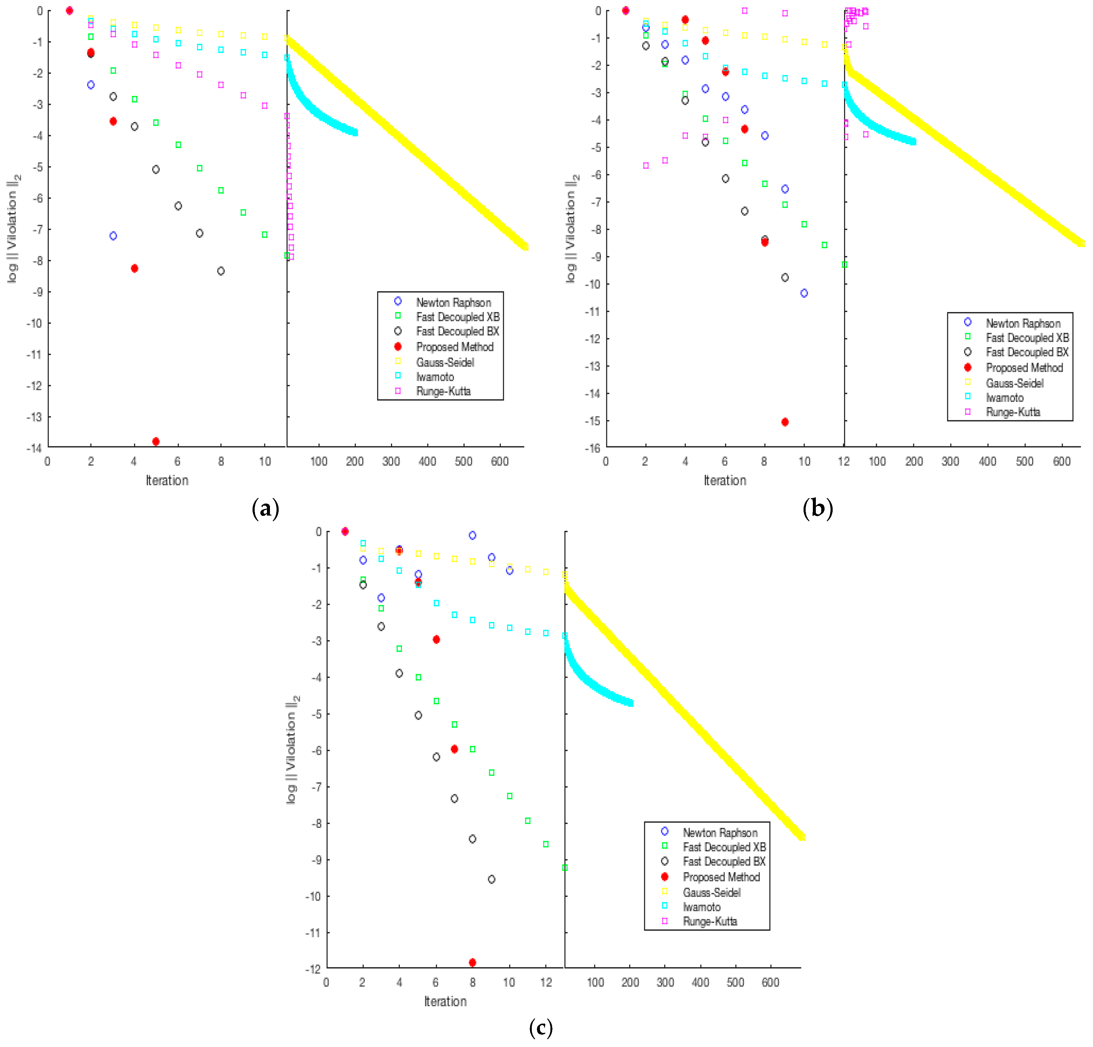
Power flow studies were performed on the IEEE 30-bus system, with various initial points $v_0={\left(1^T{0}^T\right)}^T+\beta {\left(0^T{1}^T\right)}^T$ with the range for β in [−0.3, 0.3]. A MATPOWER package [15] was used for the Newton-Raphson, fast decoupled power flow, and Gauss–Seidel methods; and a PSAT package [35] was used for the Iwamoto and Runge-Kutta methods. The same initial points were used for all methods. Figure 3 shows the results of the power flow studies: when β = 0, all of the methods converged reasonably well (Figure 3a); when β = 0.2, the Runge-Kutta method did not converge; when β = 0.3, the Runge-Kutta and Newton-Raphson methods did not converge. As mentioned in Section 2.1, Newton-Raphson method is not numerically robust. The proposed algorithm always converges rapidly in all the cases.

4.2. Optimal Power Flow Studies

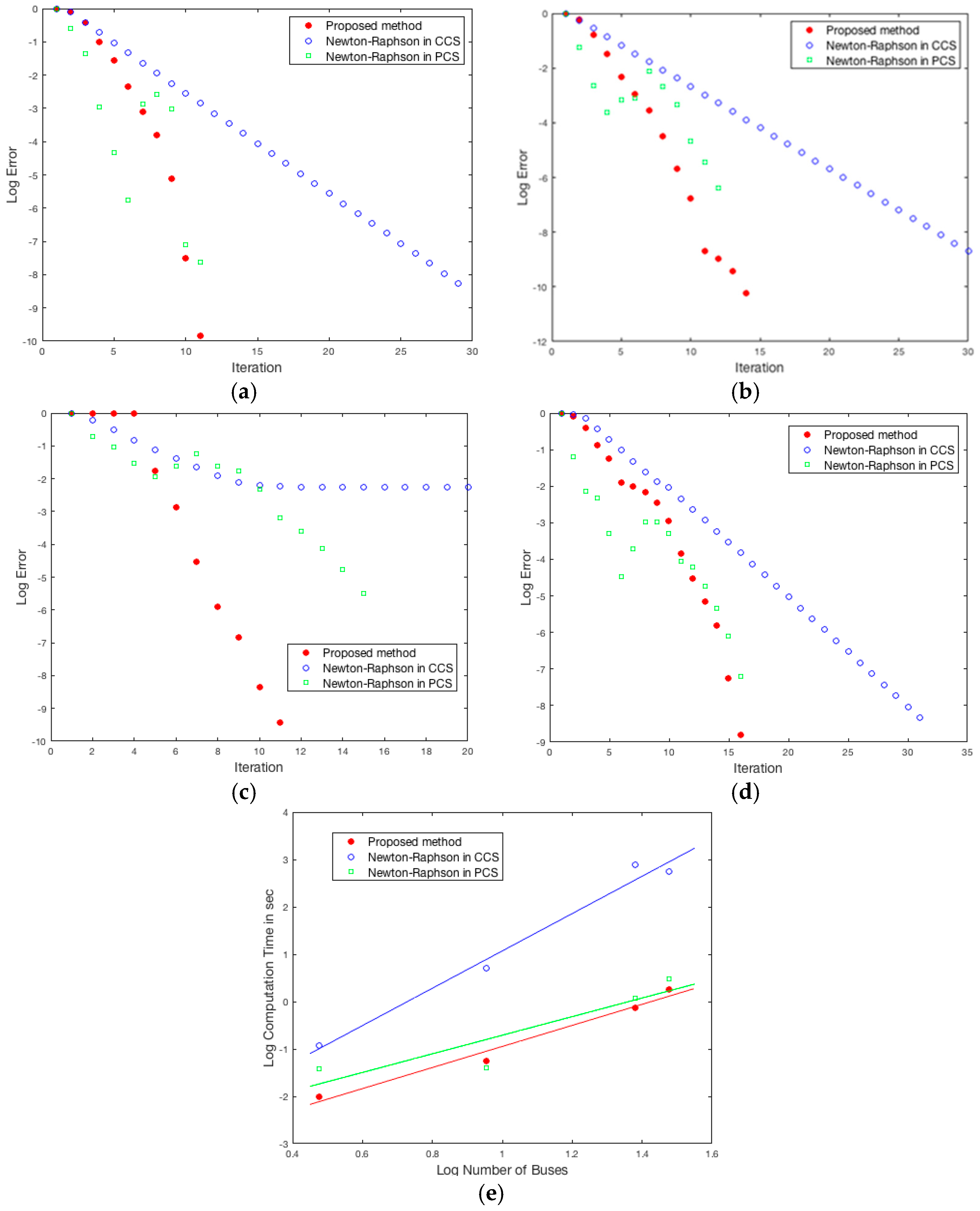
Optimal power flow studies were performed on the IEEE 3-bus, 9-bus, 24-bus, and 30-bus systems. The MIP solver in MATPOWER is based on the Newton-Raphson method formulated in the polar coordinate system (PCS), which is used for solving OPF in this study. OPF studies were performed using the proposed method and the Newton-Raphson method on the Cartesian coordinate system (CCS). Figure 4 illustrates the results. It is worthwhile to mention that structural properties of the matrices in Equation (15), such as sparsity and symmetry, are not explored yet in this study. When the structure properties are explored, it is possible to apply the proposed method for larger systems the same way as is done using the Newton-Raphson method implemented in MATPOWER.

In all the cases where the methods successfully converge, the identified solutions are identical, except for Newton-Raphson method in CCS for the IEEE-24 case (Figure 4c). For this case, the Newton-Raphson method in CCS stays at a local solution. Different from the Newton-Raphson method, the proposed method is numerically robust, and the convergence does not depend on the choice of the initial point. As shown in the computation time illustrated in the bottom plot in Figure 4, the computation time of the proposed method increases more slowly with respect to the size of the system than that of the Newton-Raphson method in CCS (p = 1.96 for the proposed method vs. 2.22 for the Newton-Raphson CCS and 1.94 for the Newton-Raphson PCS, where computation time (∝ N^p).

4.3. Probabilistic Power Flow Studies

Probabilistic power flow studies were performed on the IEEE 30-bus system. Five buses (4, 7, 16, 20, and 24) were selected for wind sites, and their wind outputs were assumed to be independent. For each wind site, the buses’ outputs were normally distributed. For the computation, the distributions were discretized into five blocks, and a probability distribution was assigned (3125 wind scenarios). The sample size for the Monte Carlo simulation (MC) was 100, and m = 2 for the 2m + 1 method [32] (Figure 5).

The computation times were 36.0, 3.26, 0.28, and 0.25 seconds for a complete search, MC, 2m + 1 method, and the proposed method, respectively. As shown in Figure 5, even for a small sample size of MC, the range of voltages and average voltages were similar to those from a complete search, but the computation cost is still large. While the 2m + 1 method reduces the cost significantly, the range and average voltages are far from those of the complete search. The proposed method yields similar voltages as from the complete search, while the computation cost is significantly reduced.

4.4. State Estimation

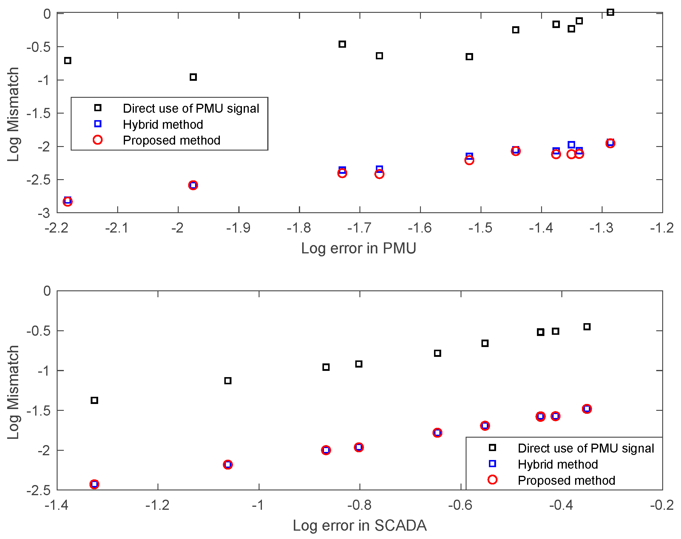
PMU and SCADA data were artificially generated with various levels of errors using an IEEE 30-bus system. For estimating the state, three methods were applied: (1) direct use of a PMU signal, in which voltages at the buses observed by PMU are directly computed, and those at other buses are estimated with SCADA; (2) a hybrid method based on the Newton–Raphson method; and (3) the proposed method (Figure 6). The methods to utilize both signals simultaneously outperformed the direct use of PMU signal.

5. Conclusions

A unified formulation based on a Kronecker product for full AC power flow studies is proposed. The solution algorithm and the proof of convergence are presented, and its performance on the studies are compared against those of conventional methods. Future work will explore the structural properties of the matrix associated with the bilinear least-square problem. Since the matrix is sparse, like that used in the Newton-Raphson method, and has a similar symmetric structure, the computation time would decrease accordingly.

References

- Grainger, J.; Stevenson, W., Jr. Power System Analysis; McGraw-Hill: New York, NY, USA, 1994; pp. 655–664. [Google Scholar]
- Morales, J.; Baringo, L.; Conejo, A.; Minguez, R. Probabilistic power flow with correlated wind sources. IET Gener. Transm. Distrib. 2010, 4, 641–651. [Google Scholar] [CrossRef] [Green Version]
- Constantinescu, E.; Zavala, V.; Rocklin, M.; Lee, S.; Anitescu, M. A computational framework for uncertainty quantification and stochastic optim-ization in unit commitment with wind power generation. IEEE Trans. Power Syst. 2011, 26, 431–441. [Google Scholar] [CrossRef]
- Borkowska, B. Probabilistic load flow. IEEE Trans. Power Apparatus Syst. 1974, PAS-93, 752–755. [Google Scholar] [CrossRef]
- Allan, R.; Borkowska, B.; Grigg, C. Probabilistic analysis of power flows. Proc. Inst. Electr. Eng. 1974, 121, 1551–1556. [Google Scholar] [CrossRef]
- Silva, A.; Ribeiro, S.; Arienti, V.; Allan, R.; Filho, M. Probabilistic load flow techniques applied to power system expansion planning. IEEE Trans. Power Syst. 1990, 5, 1047–1053. [Google Scholar] [CrossRef]
- Chen, P.; Chen, Z.; Bak-Jensen, B. Probabilistic load flow: A review. In Proceedings of the 2008 Third International Conference on Electric Utility Deregulation and Restructuring and Power Technologies, Nanjing, China, 6–9 April 2008. [Google Scholar]
- Prusty, B.; Jena, D. A Critical Review on Probabilistic Load Flow Studies in Uncertainty Constrained Power Systems with Photovoltaic Generation and a New Approach. Renew. Sustain. Energy Rev. 2017, 69, 1286–1302. [Google Scholar] [CrossRef]
- Carpentier, J. Contribution to the economic dispatch problem. Bull. Soc. Fr. Des Electr. 1962, 3, 431–447. [Google Scholar]
- Huneault, M.; Galiana, F.D. A survey of the optimal power flow literature. IEEE Trans. Power Syst. 1991, 6, 762–770. [Google Scholar] [CrossRef]
- Momoh, J.A.; El-Hawary, M.E.; Adapa, R. A review of selected optimal power flow literature to 1993. Part I: Nonlinear and quadratic programming approaches. IEEE Trans. Power Syst. 1999, 14, 96–104. [Google Scholar] [CrossRef]
- Momoh, J.A.; El-Hawary, M.E.; Adapa, R. A review of selected optimal power flow literature to 1993. Part II: Newton, linear programming and interior point methods. IEEE Trans. Power Syst. 1999, 14, 105–111. [Google Scholar] [CrossRef]
- Pandya, K.S.; Joshi, S.K. A survey of optimal power flow methods. J. Theor. Appl. Inf. Technol. 2008, 4, 450–458. [Google Scholar]
- Jiang, Q.Y.; Chiang, H.D.; Guo, C.X.; Cao, Y.J. Power-current hybrid rectangular formulation for interior-point optimal power flow. IET Gener. Transm. Distrib. 2009, 3, 748–756. [Google Scholar] [CrossRef]
- Wang, H.; Murillo-Sanchez, C.E.; Zimmerman, R.D.; Thomas, R.J. On computational issues of market-based optimal power flow. IEEE Trans. Power Syst. 2007, 22, 1185–1193. [Google Scholar] [CrossRef]
- Schellenberg, A.; Rosehart, W.; Aguado, J. Cumulant-based probabilistic optimal power flow (P-OPF) with Gaussian and gamma distributions. IEEE Trans. Power Syst. 2005, 20, 773–781. [Google Scholar] [CrossRef]
- Roa-Sepulveda, C.A.; Pavez-Lazo, B.J. A solution to the optimal power flow using simulated annealing. Int. J. Electr. Power Energy Syst. 2003, 25, 47–57. [Google Scholar] [CrossRef]
- Verbic, G.; Schellenberg, A.; Rosehart, W.; Canizares, C.A. Probabilistic Optimal Power Flow applications to electricity markets. In Proceedings of the 2006 International Conference on Probabilistic Methods Applied to Power Systems, Stockholm, Sweden, 11–15 June 2006. [Google Scholar]
- Chen, L.; Suzuki, H.; Katou, K. Mean field theory for optimal power flow. IEEE Trans. Power Syst. 1997, 12, 1481–1486. [Google Scholar] [CrossRef]
- Liu, L.; Wang, X.; Ding, X.; Chen, H. A robust approach to optimal power flow with discrete variables. IEEE Trans. Power Syst. 2009, 24, 1182–1190. [Google Scholar] [CrossRef]
- Gopalakrishnan, A.; Raghunathan, A.U.; Nikovski, D.; Biegler, L.T. Global optimization of optimal power flow using a Branch & Bound algorithm. In Proceedings of the 2012 50th Annual Allerton Conference on Communication, Control, and Computing, Monticello, IL, USA, 1–15 October 2012. [Google Scholar]
- Tawarmalani, M.; Sahinidis, N.V. A polyhedral branch-and-cut approach to global optimization. Math. Program. 2005, 103, 225–249. [Google Scholar] [CrossRef]
- Bai, X.; Wei, H.; Fujisawa, K.; Wang, Y. Semidefinite programming for optimal power flow problems. Int. J. Electr. Power Energy Syst. 2008, 30, 383–392. [Google Scholar] [CrossRef]
- Lavaei, J.; Low, S.H. Zero duality gap in optimal power flow. IEEE Trans. Power Syst. 2012, 27, 92–106. [Google Scholar] [CrossRef]
- Lesieutre, B.; Molzahn, D.; Borden, A.; DeMarco, C.L. Examining the limits of the application of semidefinite programming to power flow problems. In Proceedings of the 2011 49th Annual Allerton Conference on Communication, Control, and Computing, Monticello, IL, USA, 28–30 September 2011; pp. 1492–1499. [Google Scholar]
- Josz, C.; Maeght, J.; Panciatici, P.; Gilbert, J. Application of the Moment-SOS approach to Global Optimization of the OPF problem. IEEE Trans. Power Syst. 2015, 30, 463–470. [Google Scholar] [CrossRef]
- Trias, A. The Holomorphic Embedding Load Flow Method. In Proceedings of the 2012 IEEE Power and Energy Society General Meeting, San Diego, CA, USA, 22–26 July 2012. [Google Scholar]
- Bakirtzis, A.; Biskas, P.; Zoumas, C. Optimal power flow by enhanced genetic algorithm. IEEE Trans. Power Syst. 2002, 17, 229–236. [Google Scholar] [CrossRef]
- Abido, M. Optimal power flow using particle swam optimization. Int. J. Electr. Power Energy Syst. 2002, 24, 563–571. [Google Scholar] [CrossRef]
- Kuhn, H.; Tucker, A. Nonlinear programming. In Proceedings of the 2nd Berkeley Symposium on Mathematical Statistics and Probability, Berkeley, CA, USA, 31 July–12 August 1950; University of California Press: Berkeley, CA, USA, 1951; pp. 481–492. [Google Scholar]
- Golub, G.H.; van Loan, C.F. Matrix Computations, 4th ed.; Johns Hopkins University Press: Baltimore, MD, USA, 2012. [Google Scholar]
- Su, C. Probabilistic load-flow computation using point estimate method. IEEE Trans. Power Syst. 2005, 20, 1843–1851. [Google Scholar] [CrossRef]
- Nuqui, R.; Phadke, A. Hybrid Linear State Estimation Utilizing Synchronized Phasor Measurements. In Proceedings of the 2007 IEEE Lausanne Power Tech, Lausanne, Switzerland, 1–5 July 2007; pp. 1665–1669. [Google Scholar]
- Chakrabarti, S.; Kyriakides, E.; Ledwich, G.; Ghosh, A. A Comparative Study of the Methods of Inclusion of PMU Current Phasor Measurements in a Hybrid State Estimator. In Proceedings of the IEEE Power and Energy Society General Meeting, Providence, RI, USA, 25–29 July 2010; pp. 1–7. [Google Scholar]
- Milano, F. Power System Analysis Toolbox. Available online: http://faraday1.ucd.ie/psat.html (accessed on 20 June 2019).
Figure 1.
The comparison of the performance: ALS (triangle), modified ALS (square), and proposed algorithm (circle).
Figure 2.
Comparison in the convergences of the Newton-Raphson method and proposed methods.
Figure 3.
Performances of the Newton–Raphson, fast decoupled power flow, Gauss-Seidel, Runge-Kutta, Iwamoto, and proposed methods to solve power flow problems on an IEEE 30-bus system. Variable ε in the y-axis is the mismatch in power balance or voltage magnitude. (a) β = 0.0; (b) β = 0.2; (c) β = 0.3 in v0 = (1T 0T)T + β(0T 1T)T.
Figure 4.
Performances of the Newton-Raphson method formulated in the polar coordinate system (PCS) (green square), of the Newton-Raphson method formulated in the Cartesian coordinate system (CCS; blue circle), and of the proposed method (red circle) for IEEE model systems; 3-bus (a); 9-bus (b); 24-bus (c); and 30-bus systems (d); as well as the computation times of the algorithms (e).
Figure 5.
Probabilistic power flow results: (top) real parts of voltages and (bottom) imaginary parts of voltages. Black line: complete search; blue line: Monte Carlo simulation; green line: 2m + 1 method; and red line: proposed method.
Figure 6.
Performances of the state estimators with various measurement errors; (top) errors from PMU (phasor measurement unit) measurements, and (bottom) errors from SCADA (supervisory control and data acquisition) measurements.
© 2019 by the author. Licensee MDPI, Basel, Switzerland. This article is an open access article distributed under the terms and conditions of the Creative Commons Attribution (CC BY) license (http://creativecommons.org/licenses/by/4.0/).
Share and Cite
MDPI and ACS Style
Oh, H. A Unified and Efficient Approach to Power Flow Analysis. Energies 2019, 12, 2425. https://doi.org/10.3390/en12122425
AMA Style
Oh H. A Unified and Efficient Approach to Power Flow Analysis. Energies. 2019; 12(12):2425. https://doi.org/10.3390/en12122425
Chicago/Turabian StyleOh, HyungSeon. 2019. "A Unified and Efficient Approach to Power Flow Analysis" Energies 12, no. 12: 2425. https://doi.org/10.3390/en12122425
Note that from the first issue of 2016, this journal uses article numbers instead of page numbers. See further details here.