Exploring Economic Criteria for Energy Storage System Sizing

Abstract

This paper presents two economic criteria for guiding the energy storage system (ESS) sizing in grid-connected microgrids. The internal power output model and the economic operation model of ESS are firstly established. Then, the combination of heuristic adjustment strategy and hybrid particle swarm optimization algorithm are introduced to solve the optimal operation model of ESS. Then according to the ESS life model and cost-benefit analysis, a static investment economic criterion which is easy and simple to be calculated is proposed to demonstrate the economic feasibility of ESS investment programs in the short term. Considering the time value of currency, a dynamic investment economic criterion is proposed later for long-term investment projects. Furthermore, the ESS sizing boundary of achieving profits could be also obtained according to the criteria which can indicate the economic attractiveness or resistance to ESS investors in the microgrid. A case study has verified its effectiveness. At the same time, sensitivity analysis is given to show the impact on key parameters, such as investment unit price and electricity purchase price on ESS investment.

1. Introduction

Variable renewable energy (VRE), e.g., wind turbine (WT) power generation and photovoltaic (PV) power generation, is characterized by intermittence, randomness, and uncertainties. As the VRE penetration rate continues to increase, high-proportion VRE generation has become a global concern for the future power system scenario. In the new scenario, the characteristics of power systems have changed dramatically, and the integration of large-scale VRE has brought more and more challenges to the safe and reliable operation of the power grid. To solve this problem, energy storage technology has been extensively studied as an effective means to mitigate the fluctuation of VRE generation.

Energy storage technology has been recognized as an important part in system operation. After the introduction of energy storage in the system, the demand side management can be effectively realized, the peak-to-valley difference at night can be eliminated, and the load can be smoothed. Energy storage technology can not only utilize the power equipment more effectively and reduce the power supply cost, but also promote the application of renewable energy. Besides, it can also be used as a means to improve system operation stability, adjust frequency, and compensate for load fluctuations. For decades, the research and development of energy storage technology has been valued by the energy, transportation, electric power, telecommunication, and other departments of various countries. The application of energy storage technology will bring major changes in the design, planning, scheduling, and control of traditional power systems [1]. Data from the DOE Global Energy Storage Database show that by the end of June 2018, the cumulative installed capacity of energy storage projects worldwide was 195.74 GW. From 1997 to 2017, the installed capacity of energy storage systems in the world increased by 70%. The United States, China, and Japan lead the global market. Nowadays, the energy storage market has been developed positively under the policy encouragement of governments. In recent years, new energy storage projects and their total installed capacity are expected to increase several times.

Existing research and practices have shown that the integration of various distributed energy resources in the form of microgrids is an effective way to fully utilize the diversity of power supply performance. A microgrid refers to a small-scale power distribution system that is a collection of distributed power sources, energy storage devices, energy conversion devices, related loads, and monitoring and protection devices. It is an autonomous system that can achieve self-control, protection, and management. It can be also operated in parallel with the external power grid. From the perspective of the grid, the biggest advantage of the microgrid is that it integrates all the components into a controllable whole in a systematic way. From the user’s point of view, the biggest advantage of the microgrid is that as an autonomous operating power system, it can provide users with customizable power to meet the power quality and reliability requirements of different users. From an environmental point of view, microgrids can reduce heat pollution caused by pollutants, greenhouse gas emissions, and waste heat. In view of the huge economic and social benefits of microgrids, more and more microgrid laboratories and demonstration projects are being carried out at home and abroad [2].

In recent years, energy storage has been widely studied and utilized in the microgrid, in which distributed renewable generations (DRGs) are highly penetrated and integrated with other resources [3]. In microgrids, energy storage could help realize power peak-shaving and enhance the reliability of power supply due to the uncertainty of DRGs outputs [4,5,6]. Thus, more energy storage should be introduced into the emerging user side microgrids, e.g., industry parks and residential communities, [7] to improve the operation performance of the power system. However, expensive investment of the energy storage system (ESS) limits its sizing in microgrids [8]. How to determine an effective ESS sizing program to achieve the equilibrium between its cost in the investment/operation process and corresponding economic benefits is eager to be solved.

Various methods were proposed for the sizing of ESS. For instance, a Fourier–Legendre series based optimal model was designed for the economic operational behavior of ESS sizing [9]. The value of battery energy storage in shifting wind generation from off-peak to on-peak periods and limiting the ramp rate of wind farm output was investigated in [10] and utilized in the optimization. In [11], factors such as energy storage arbitrage income, government electricity price subsidy income, reduction of electricity transfer costs, delays in grid upgrades, and full life cycle costs are considered in the model. In [12], the ESS optimization configuration method in the wind farm station considering the energy storage life loss was proposed, combined with multi-scenario random programming and a sequential Monte Carlo simulation method. In [13], a methodology was presented to choose the proper sizing of an integrated PV unit and storage architecture starting from the knowledge of the load and solar irradiance time profiles. In [14], seven different flexible storage PV investments were analyzed in Germany, France, Italy, and Spain. To handle the uncertainty of VRE and load demand for deploying ESS, a mixed integer conic programming model was extended into a two-stage stochastic programming model in [15]. The above reference was to plan the capacity of ESS in the distribution network or with the VRE. In terms of ESS sizing in microgrids, storage types and load features were considered [16], DRG deployments were integrated [17], while the demand response strategy of available controllable elements was designed [18] in the sizing modeling. In [19], the unit commitment problem with spinning reserve for microgrids was considered in the sizing method. In [20], a two-layer optimization model of microgrid ESS capacity considering both economic operation and battery life was proposed to study the ESS sizing problem. Furthermore, a robust metaheuristic optimization algorithm, called evolutionary particle swarm optimization, was employed to solve sizing problems in a standalone microgrid [21]. The benefits of investing ESS is close to the power exchange between the microgrid and the main grid, thus the grid-connected mode is the focus of this paper. On the other hand, Reference [22] reviews the existing ESS sizing methods for microgrid applications and presents a generic sizing method that enables microgrid planners to efficiently determine the optimal ESS size, technology, and location. However, cost-benefit analysis was seldom investigated in the above ESS investment studies.

It could be seen from above that most existing studies on ESS sizing in microgrids mainly focused on the comprehensive sizing of various types of power supplies in microgrid systems or the solution of the optimal capacity of ESS. These studies were insufficient in considering the case of investing ESS in an existing microgrid and the complete economic analysis for it. The majority of them were mainly from the view of the microgrid operator in order to minimize the total cost, which is not from the view of the ESS investor and cannot effectively reflect economic feasibility of ESS investment behavior. The incurred consequence is that the integration of ESS might be unprofitable in microgrids. From the point of view of an ESS investor, more attention was paid to the direct economic benefits of investing in ESS rather than other indirect benefits which cannot be reflected in their cash flow. Similar to the economic criterion for DRG planning [23], a simple economic criterion for indicating the economic feasibility of ESS deployment and optimal sizing in microgrids is also vital. Meanwhile, few studies analyzed the boundaries between the profitability and unprofitability of ESS investments generated as the capacity increases due to microgrid size constraints. In order to more effectively and quickly clarify the economic feasibility of the ESS integration in a grid-connected microgrid, this paper innovatively designs two economic criteria to indicate the profit of ESS integration. Not only optimal capacity but also profit boundary can be found and a lot of economic analyses are given. The main contributions of the paper are as follows:

(1) The ESS economic operation model based on time-of-use (TOU) electricity price is established to determine the benefit of the energy storage system. Additionally, an improved hybrid particle swarm algorithm is proposed to solve the ESS economic operation model.

(2) Taking into account the life cycle of ESS, the static investment economic criterion is proposed to indicate the economic feasibility of integrating ESS during the life cycle of the energy storage device.

(3) Considering the time value of currency, the dynamic investment economic criterion is proposed to indicate the economic feasibility during the predefined project life cycle.

(4) A method for the sizing and the profit boundary determination of ESS integration is presented based on the proposed criteria, which can help guide the investment behavior of ESS integration.

The rest of the paper is as follows: In Section 2, the distributed power model of the microgrid and the economic operation model of ESS are established. And the solution method for solving the economic operation model is introduced. Then the ESS life model and the static and dynamic investment economic criteria are presented later. The case studies are presented in Section 3 and the conclusions are summarized in Section 4.

2. Materials and Methods

2.1. Power Supply Model of the Microgrid

A microgrid is an effective technical means for efficient management and comprehensive utilization of renewable energy. It includes parts such as power, load, and control systems. Among them, the power supply of the microgrid studied in this paper is composed of WT power, PV power, and an energy storage system. Assume that the microgrid is connected to the upper grid so that the upper grid can supply power to the microgrid. Therefore, the supply to relevant loads in the microgrid is realized by four methods: WT power, PV power, energy storage system, and power purchase from the upper grid.

2.1.1. Modeling of WT Power

Wind energy as a clean energy source to generate electricity can indeed reduce environmental pollution, but WT output is strongly affected by wind speed changes so that it is characterized by intermittence and volatility. Therefore, wind speed prediction plays a key role in WT power forecasting of the power system. In addition, a lot of research shows the WT output can be considered as a function of wind velocity [24]. A piecewise function can be used to fit the relationship between the output power and wind speed as shown below.

$$P_{\mathrm{W}}=\{\begin{array}{cc}0& 0\le v\le v_{ci}\mathrm{or}v\ge v_{co}\\ P_r\frac{(v-v_{ci})}{(v_r-v_{ci})}& v_{ci}\le v\le v_r\\ P_r& v_r\le v\le v_{co}\end{array},$$

(1)

where $P_{\mathrm{W}}$ is the WT output power. $P_r$ is the rated power of WT. $v$ is the wind speed. $v_{ci}$, $v_{co}$, and $v_r$ are the cut-in wind speed, the cut-off wind speed, and the rated wind speed, respectively.

2.1.2. Modeling of PV Power

There are many environmental factors affecting the output of PV systems, such as solar radiation, temperature, dust, etc. In order to simplify the complexity of the problem, only the main factors of solar radiation are considered to establish the PV output model. For achieving high energy transfer efficiency, the PV should work at the maximum power point. In the PV module, we assume that a maximum power point tracker will be used. The PV power output is formulated as Equation (2) [25].

$$P_{\mathrm{PV}}=\eta SI(1-0.005(t_0-25)),$$

(2)

where $P_{\mathrm{PV}}$ is the PV output power. $\eta$ is the conversion efficiency of the solar cell array. $S$ is the array area. $I$ is the solar radiation. $t_0$ is the outside air temperature.

2.1.3. Modeling of ESS

ESS is an important part of a microgrid. The ESS with a certain capacity in a microgrid has many functions. On the one hand, ESS can effectively stabilize the fluctuation of renewable energy generation power in microgrids and improve power quality. On the other hand, ESS can also adjust the system load peak-to-valley difference to obtain economic benefits. In addition, ESS can also be used as a backup power supply for the system in an emergency, ensuring the reliability of the system operation. During operation, the charging power and discharging power of the ESS can be respectively presented by Equations (3) and (4) [19].

$$P_{\mathrm{ESS},t}^{\mathrm{ch}}=(E_t-E_{t-1})/{\eta }_{\mathrm{ch}}\Delta t,$$

(3)

$$P_{\mathrm{ESS},t}^{\mathrm{dis}}=(E_{t-1}-E_t){\eta }_{\mathrm{dis}}/\Delta t,$$

(4)

where $P_{\mathrm{ESS},t}^{\mathrm{ch}}$ and $P_{\mathrm{ESS},t}^{\mathrm{dis}}$ are the charging power and discharging power at time t. $E_t$ and $E_{t-1}$ are the state of charge (SOC) of ESS at time t and time t − 1. ${\eta }_{\mathrm{ch}}$ and ${\eta }_{\mathrm{dis}}$ are the charging efficiency and discharging efficiency of ESS. $\Delta t$ is the time interval which is 1 h in this paper.

2.2. ESS Economic Operation Model

2.2.1. Objective Function

The benefits generated by ESS depend on the operating mode, which consist of peak-shaving, smoothing renewable energy fluctuation, frequency adjustment, and system backup, etc. In different modes, the benefits vary. When the ESS is used as a system backup, it can bring environmental benefits by replacing the thermal power unit. When the ESS is used for peak-shaving in the distribution network, it can play a role in delaying the upgrade of the distribution network. In this paper, ESS is used to store electricity during the valley period and supply electricity during the peak period. Assume that TOU price is implemented and the microgrid cannot reverse power to the upper grid. The economic operation model aiming at maximizing the operational benefits of integrating ESS in a scheduling cycle can be formulated as:

Maximize:

$$I_{\mathrm{up}}={\displaystyle \sum _{t=1}^T(P_{\mathrm{B},t}-P_{\mathrm{ES},\mathrm{B},t})}\cdot {\lambda }_t,$$

(5)

where T represents the hours of a scheduling cycle. Respectively, $P_{\mathrm{B},t}$ and $P_{\mathrm{E}\mathrm{S},\mathrm{B},t}$ represent the power purchase from the upper grid at time t without and with ESS. ${\lambda }_t$ is the electricity price presented by Equation (6).

$${\lambda }_t=\{\begin{array}{c}{\lambda }_{\mathrm{p}},t\in {\mathsf{\Omega }}_{\mathrm{p}}\\ {\lambda }_{\mathrm{n}},t\in {\mathsf{\Omega }}_{\mathrm{n}}\\ {\lambda }_{\mathrm{v}},t\in {\mathsf{\Omega }}_{\mathrm{v}}\end{array},$$

(6)

where ${\lambda }_{\mathrm{p}}$, ${\lambda }_{\mathrm{n}}$, and ${\lambda }_{\mathrm{v}}$ are the values of electricity price during peak, normal, and valley periods represented by ${\mathsf{\Omega }}_{\mathrm{p}}$, ${\mathsf{\Omega }}_{\mathrm{n}}$, and ${\mathsf{\Omega }}_{\mathrm{v}}$.

2.2.2. Constraints

The basic constraints for the economic operation model are listed as follows.

(1) Power balance equation:

$$P_{\mathrm{W},t}+P_{\mathrm{PV},t}+P_{\mathrm{ESS},t}^{\mathrm{dis}}+P_{\mathrm{ES},\mathrm{B},t}=P_{\mathrm{Load},t}+P_{\mathrm{ESS},t}^{\mathrm{ch}},$$

(7)

where $P_{\mathrm{W},t}$ and $P_{\mathrm{PV},t}$ are, respectively, the output of the WT power and the PV power at time t. $P_{\mathrm{Load},t}$ represents the load power at time t.

(2) Charging and discharging power constraint:

$$0<P_{\mathrm{ESS},t}^{\mathrm{ch}}<P_{\mathrm{ESS},\max }^{\mathrm{ch}},$$

(8)

$$0<P_{\mathrm{ESS},t}^{\mathrm{dis}}<P_{\mathrm{ESS},\max }^{\mathrm{dis}},$$

(9)

where $P_{\mathrm{ESS},\max }^{\mathrm{ch}}$ and $P_{\mathrm{ESS},\max }^{\mathrm{dis}}$ represents the maximum charging and discharging power.

(3) ESS state of charge (SOC) constraint:

$$E_{\min }<E_t<E_{\max },$$

(10)

where $E_{\min }$ and $E_{\max }$ are the minimum and maximum values of SOC.

In the regional power grid, the scheduling of the ESS also has periodicity, that is, the SOC at the start of the scheduling period and the SOC at the end of the scheduling period should satisfy the following constraints.

$$E_{t^{\mathrm{start}}}=E_{t^{\mathrm{end}}}=E_{\mathrm{initial}},$$

(11)

where $E_{t^{\mathrm{start}}}$ and $E_{t^{\mathrm{end}}}$ respectively represent the SOC of the ESS at the start and the end of the scheduling period. $E_{\mathrm{initial}}$ is the initial set value of SOC.

2.3. Improved Hybrid Particle Swarm Optimization for Solving the Economic Operation Model

The ESS economic operation model is complicated to solve, and it is difficult to find the theoretical optimal solution. The existing literature has tried various methods, such as the Lagrangian relaxation method [26], the genetic algorithm [27], and the particle swarm optimization (PSO) algorithm [28]. Among them, the PSO algorithm is widely used in such problems because of its easy implementation, high precision, and fast convergence. Focusing on the problem that particle swarm optimization easily falls into the local optimal solution, this paper uses the improved hybrid PSO algorithm in [29] to solve the economic operation model of ESS.

For the traditional PSO algorithm, suppose that there are N particles forming a population in the M-dimensional search space. Each particle is a T-dimensional vector representing the position of the particle in the T-dimensional search space, which is a potential solution to the problem. According to the objective function, the fitness value corresponding to each particle position can be calculated, and its size indicates the quality of the particle. Through continuous iteration, the particles move in the solution space to achieve optimization. During each iteration, the particle’s position and velocity are updated based on individual extremum and population extremum as shown in Equations (12) and (13) [29].

$$V_{id}^{k+1}=\omega V_{id}^k+c_1{r}_1(P_{id}^k-X_{id}^k)+c_2{r}_2(P_{gd}^k-X_{id}^k),$$

(12)

$$X_{id}^{k+1}=X_{id}^k+V_{id}^{k+1},$$

(13)

where $\omega$ is the inertia weight. d = 1, 2, …, M. i = 1, 2, …, N. k is the current iterations. $V_{id}^{k+1}$ and $V_{id}^k$ are the particle velocity of the k+1th iteration and the kth iteration. $X_{id}^{k+1}$ and $X_{id}^k$ are the particle position of the k+1th iteration and the kth iteration. $P_{id}^k$ and $P_{gd}^k$ are the individual extremum and population extremum of the kth iteration. $c_1$ and $c_2$ are non-negative constants called acceleration factors. $r_1$ and $r_2$ are random numbers distributed in the interval [0, 1].

In order to prevent a blind search of particles, the particle position and velocity should meet the following constraints.

$$-X_{\max }\le X_{id}^k\le X_{\max },$$

(14)

$$-V_{\max }\le V_{id}^k\le V_{\max },$$

(15)

where $X_{\max }$ and $V_{\max }$ are the maximum particle position and velocity.

However, the charging and discharging process of the ESS is limited by SOC and charging and discharging power. Furthermore, there is a coupling relationship between the time periods. These reasons lead to the complexity of the constraints of the economic operation model. The result is a lower probability of obtaining a feasible solution, which limits the efficiency of the PSO algorithm. To this end, a heuristic adjustment strategy of charging and discharging and the hybrid PSO algorithm are adopted in this paper. The SOC of the ESS is adjusted by the forward-backward sweep method to satisfy all the constraints, increase the probability of the feasible solution, and improve the performance of the algorithm.

The specific steps of solving are as follows:

• Enter the WT power, and PV power and load profiles.
• Initialize the SOC of ESS during each period.
• Use the heuristic charging and discharging adjustment strategy of the ESS to adjust its charge and discharge behavior to meet the constraints and ensure the power balance of the entire microgrid system. Details are as follows:
  • Judge whether or not the SOC $E_t$ of the ESS exceeds the limit. If the maximum value $E_{\max }$ is exceeded, $E_t$ is taken as $E_{\max }$. If $E_t$ is lower than the minimum value $E_{\min }$, it is taken as $E_{\min }$.
  • Let t = 2, …, T. If the adjacent period satisfies Equation (16), adjust the $E_t$ by Equation (17). If the adjacent period satisfies Equation (18), adjust the $E_t$ by Equation (19).

    $$E_t>E_{t-1}+P_{\mathrm{ESS},\max }^{\mathrm{ch}}\cdot \Delta t\cdot {\eta }_{\mathrm{ch}},$$

    (16)

    $$E_t=E_{t-1}+P_{\mathrm{ESS},\max }^{\mathrm{ch}}\cdot \Delta t\cdot {\eta }_{\mathrm{ch}},$$

    (17)

    $$E_t<E_{t-1}-P_{\mathrm{ESS},\max }^{\mathrm{dis}}\cdot \Delta t/{\eta }_{\mathrm{dis}},$$

    (18)

    $$E_t=E_{t-1}-P_{\mathrm{ESS},\max }^{\mathrm{dis}}\cdot \Delta t/{\eta }_{\mathrm{dis}}.$$

    (19)
  • Judge whether or not the SOC of the start and end times of the scheduling cycle satisfies Equation (11). If the equation is satisfied, proceed to step 4. Otherwise, let () and t = T, …, 2. If the adjacent period satisfies Equation (16), adjust $E_{t-1}$ by Equation (20). If the adjacent period satisfies Equation (18), adjust $E_{t-1}$ by Equation (21).

    $$E_{t-1}=E_t-P_{\mathrm{ESS},\max }^{\mathrm{ch}}\cdot \Delta t\cdot {\eta }_{\mathrm{ch}},$$

    (20)

    $$E_{t-1}=E_t+P_{\mathrm{ESS},\max }^{\mathrm{dis}}\cdot \Delta t/{\eta }_{\mathrm{dis}}.$$

    (21)
  • Judge again whether or not Equation (11) is satisfied. If it is satisfied, proceed to step 4. Otherwise, resume step 3 again.
• Calculate the fitness value of each particle and update the individual extremum and population extremum.
• Update the particle velocity and position according to Equations (12) and (13) and perform crossover and mutation.
• Repeat steps 3, 4, and 5 until the convergence condition or maximum number of iterations is reached.

2.4. Economic Criteria for ESS Investment

Focusing on the cost-benefit analysis of ESS in microgrids, the economic criteria aim to judge whether it is economically feasible for ESS to be installed in the microgrid will be proposed in this part. The criteria are formulated based on the ESS economic operation model and are affected by the life loss of ESS.

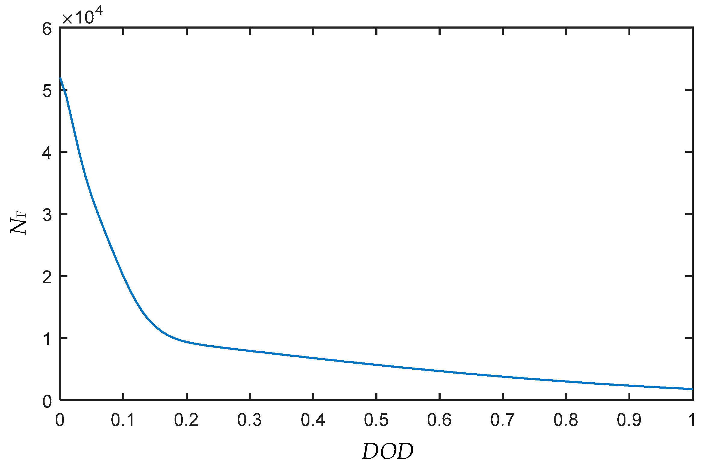
2.4.1. ESS Life Model

The service life of ESS will be affected by temperature, the power of discharging, the state transition of charging and discharging, depth of discharge, and other factors, which could be determined by the shorter one between its cycle life and float life [30]. To simplify the problem, the depth of discharging is regarded as the main factor involved in the modeling to determine the cycle life.

In a scheduling cycle, the depth of the ith discharging $DO{D}_i$ can be formulated as:

$$DO{D}_i=(E_{t^{\mathrm{start}}}^{dis,i}-E_{t^{\mathrm{end}}}^{dis,i})/S_{\mathrm{ESS}},$$

(22)

where $E_{t^{\mathrm{start}}}^{dis,i}$ and $E_{t^{\mathrm{end}}}^{dis,i}$ represent the SOC of start time and end time of ith discharging process. S_ESS is the capacity of ESS.

The cycle life of ESS can be measured in terms of the maximum number of cycles. According to the real ESS operational data and surveys [31,32], the maximum cycles N_F and DOD of the ESS could be drawn out, as one typical correlation profile shown in Figure 1. The greater the DOD, the smaller the N_F. Additionally, a certain formula reflecting the correlation relationship between those two $N_{\mathrm{F},i}=f(DO{D}_i)$ could be fitted by data mining methods.

Then, the life loss ratio of ESS in a scheduling cycle can be expressed as follows:

$$k_{\mathrm{life},T}={\displaystyle \sum _{i=1}^n{N}_{\mathrm{F},i}{}^{-1}},$$

(23)

where n is the total number of cycles in a scheduling cycle.

Suppose that ESS runs for 300 days a year. The service life of ESS can be expressed as Equation (24).

$$T_{\mathrm{S}}=\min \left\{\frac{T}{300\times 24\times k_{\mathrm{life},T}},T_{\mathrm{F}}\right\},$$

(24)

where $T_{\mathrm{F}}$ represents the ESS’s float life according to its original nameplate parameters.

2.4.2. Economic Criteria

A. Static investment economic criterion

The benefits of integrating ESS consist of two parts—government subsidies and operational benefits. The former depends on the amount of electricity generated by ESS in a scheduling cycle and is shown in Equation (25). The latter comes from the cost reduction of expensive electricity purchases, which could be obtained from the result of the ESS economic operation model. Thus, the total benefits of ESS during the life cycle of the energy storage device can be expressed as Equation (26).

$$I_{\mathrm{sub}}=k_{\mathrm{sub}}\cdot {\displaystyle \sum _{i=1}^n(E_{t^{\mathrm{start}}}^{dis,i}-E_{t^{\mathrm{end}}}^{dis,i})},$$

(25)

$$I_{\mathrm{ESS}}=\frac{300\times 24\times (I_{\mathrm{up}}+I_{\mathrm{sub}})}{T}\cdot T_{\mathrm{S}},$$

(26)

where k_sub is the coefficient of subsidies.

While calculating the benefits, the investment cost of ESS also needs to be considered. The investment cost of ESS during the life cycle of the energy storage device includes initial investment cost, and operation and maintenance costs, which are described by the following Equations.

$$C_{\mathrm{ESS}}=C_{\mathrm{IN}}+C_{\mathrm{OM}},$$

(27)

$$C_{\mathrm{IN}}=c_{\mathrm{s}}\cdot S_{\mathrm{ESS}},$$

(28)

$$C_{\mathrm{OM}}={\displaystyle \sum _{i=1}^{T_{\mathrm{S}}}{c}_{\mathrm{om}}\cdot S_{\mathrm{ESS}}},$$

(29)

where $C_{\mathrm{IN}}$ is the initial investment cost. $C_{\mathrm{OM}}$ is the operation and maintenance cost. $c_{\mathrm{s}}$ is the unit capacity price of initial investment. $c_{\mathrm{om}}$ is the unit capacity operation and maintenance price per year.

Based on the above cost-benefit analysis, the static investment economic criterion indicator $E{C}_S$ could be built as:

$$E{C}_{\mathrm{S}}=I_{\mathrm{ESS}}-C_{\mathrm{ESS}}.$$

(30)

According to the proposed, if $E{C}_{\mathrm{S}}$ > 0, the ESS is recommended to be introduced and integrated into the microgrid to improve its economic performance. It is obvious that the introduction of ESS would increase the profit. The value of $E{C}_{\mathrm{S}}$ represents the profit of ESS, which can also reflect the economic attractiveness or resistance. For example, when $E{C}_{\mathrm{S}}$ > 0, the larger $E{C}_{\mathrm{S}}$ is, the larger the profit of introducing ESS in the microgrid. Otherwise, when $E{C}_{\mathrm{S}}$ < 0, the introduction of ESS cannot bring any profit, and can even bring losses. However, it should be noted that there may exist a profit boundary with ESS investment. In that case, $E{C}_{\mathrm{S}}$ is close to 0.

B. Dynamic investment economic criterion

The static investment economic criterion is proposed for the life cycle of the energy storage device, and the dynamic investment economic criterion is for a predefined project life cycle. Furthermore, the dynamic investment economic criterion takes into account the time value of currency compared to the static investment economic criterion. It means that the current amount of money held has a higher value than the equivalent amount of money obtained in the future. Therefore, the calculation of benefits and costs will be different from the previous ones. Equations (31)–(35) show the process of establishing a dynamic investment economic criterion.

$$I_{\mathrm{ESS}}^{\prime }={\displaystyle \sum _{t=1}^{T_{\mathrm{P}}}\frac{300\times 24\times (I_{\mathrm{up}}+I_{\mathrm{sub}})}{T\cdot {(1+i)}^t}},$$

(31)

$$C_{\mathrm{ESS}}^{\prime }=C_{\mathrm{IN}}+C_{\mathrm{OM}}^{\prime }+C_{\mathrm{RE}}+C_{\mathrm{SA}},$$

(32)

$$C_{\mathrm{OM}}^{\prime }={\displaystyle \sum _{t=1}^{T_{\mathrm{P}}}\frac{c_{\mathrm{om}}\cdot S_{\mathrm{ESS}}}{{(1+i)}^t}},$$

(33)

$$C_{\mathrm{RE}}={\displaystyle \sum _{j=1}^K\frac{c_{\mathrm{re}}\cdot S_{\mathrm{ESS}}}{{(1+i)}^{j\cdot T_{\mathrm{S}}}}},$$

(34)

$$C_{\mathrm{SA}}=\frac{T_{\mathrm{P}}\%T_{\mathrm{S}}\cdot c_{\mathrm{re}}\cdot S_{\mathrm{ESS}}}{T_{\mathrm{S}}\cdot {(1+i)}^{T_{\mathrm{P}}}},$$

(35)

where $T_{\mathrm{P}}$ is a predefined project engineering cycle. $i$ is the discount rate. $C_{\mathrm{RE}}$ is the renewal cost of the energy storage device. $C_{\mathrm{SA}}$ is the residual value of the energy storage device at the end of the project cycle. $c_{\mathrm{re}}$ is the unit capacity update cost of the energy storage device. K is the number of energy storage device updates.

Thus, the dynamic investment economic criterion indicator $E{C}_{\mathrm{D}}$ could be built as:

$$E{C}_{\mathrm{D}}=I_{\mathrm{ESS}}^{\prime }-C_{\mathrm{ESS}}^{\prime }.$$

(36)

Similar to the static investment economic criterion, the dynamic investment economic criterion is also used to judge the economic feasibility of integrating ESS. The difference is that the dynamic investment economic criterion takes into account the time value of currency and focuses on the economic feasibility of the entire investment project cycle. If $E{C}_{\mathrm{D}}$ > 0, the investment project is considered to be economically viable. On the contrary, the investment project is not recommended, although the benefit is greater than the cost apparently.

3. Results and Discussion

A local microgrid was utilized as the test system, in which PV and WT units were installed inside. The scheduling cycle was set as 24 h. Let N_F = 23390exp(−(((100DOD + 2) − 0.6852)/3.949)²) + 21830exp(−(((100DOD + 2) − 4.679)/8.114)² + 14580exp(−(((100DOD + 2) + 49.69)/105)²). The parameters of ESS in the base case were set as shown in

Table 1. Parameters of the energy storage system (ESS).

Parameter Type	Parameter Value	Parameter Type	Parameter Value
$S_{\mathrm{ESS}}$	1000 kWh	$c_{\mathrm{s}}$	1500 yuan/kWh
$P_{\mathrm{ESS},\max }^{\mathrm{ch}}$	200 kW	$P_{\mathrm{ESS},\max }^{\mathrm{dis}}$	200 kW
$E_{\max }$	1000 kWh	$E_{\min }$	300 kWh
$E_{\mathrm{initial}}$	300 kWh	$k_{\mathrm{sub}}$	0.3 yuan/kWh
$T_{\mathrm{F}}$	6a	$c_{\mathrm{om}}$	30 yuan/kWh
${\eta }_{\mathrm{ch}}$	0.85	${\eta }_{\mathrm{dis}}$	0.85

. Based on historical wind speed, solar radiation, and load data, a typical operational scenario with selected WT power, PV power, and load profiles are provided in Figure 2, according to Equations (1) and (2). In Figure 2, it can be seen that WT power and PV power cannot fully meet the load demand so that the microgrid needs to purchase power from the upper grid. For example, when t = 18 h, the co-output is 298 kW, which is lower than the load demand (747 kW). This provides a feasible space for the integration of ESS, that is, charging when the electricity price is low, and discharging when the electricity price is high to meet the load demand instead of purchasing. The ESS economic operation model was solved by the improved hybrid PSO algorithm proposed in Section 2 on the MATLAB platform. Let N = 200, $c_1$ = 2.0, $c_2$ = 2.0, ω = 0.7298, the maximum number of iterations is 150.

3.1. The Base Case

As ESS with a certain capacity (1000 kWh), the simulation result of ESS is shown in Figure 3, as the local electricity price shown together. It can be observed that the ESS is charged and discharged twice in one day, and the depth of discharge is 70%, which is the maximum each time. In addition, compared with Figure 3, it can be observed more clearly that ESS is charged in valley or normal periods and discharged in peak periods to gain benefits from the price difference in Figure 4, which verify the effectiveness of the proposed algorithm. For example, when t = 10 h, that electricity price is in peak period, the SOC curve is falling in Figure 4, and ESS is discharging in Figure 3. In the base case, the static investment economic criterion $E{C}_{\mathrm{S}}$ = 135,856.94 yuan, i.e., $E{C}_{\mathrm{S}}$ > 0. It indicates that more economic benefits could be obtained compared with its cost by investing 1000 kWh in the local microgrid with the setting parameters.

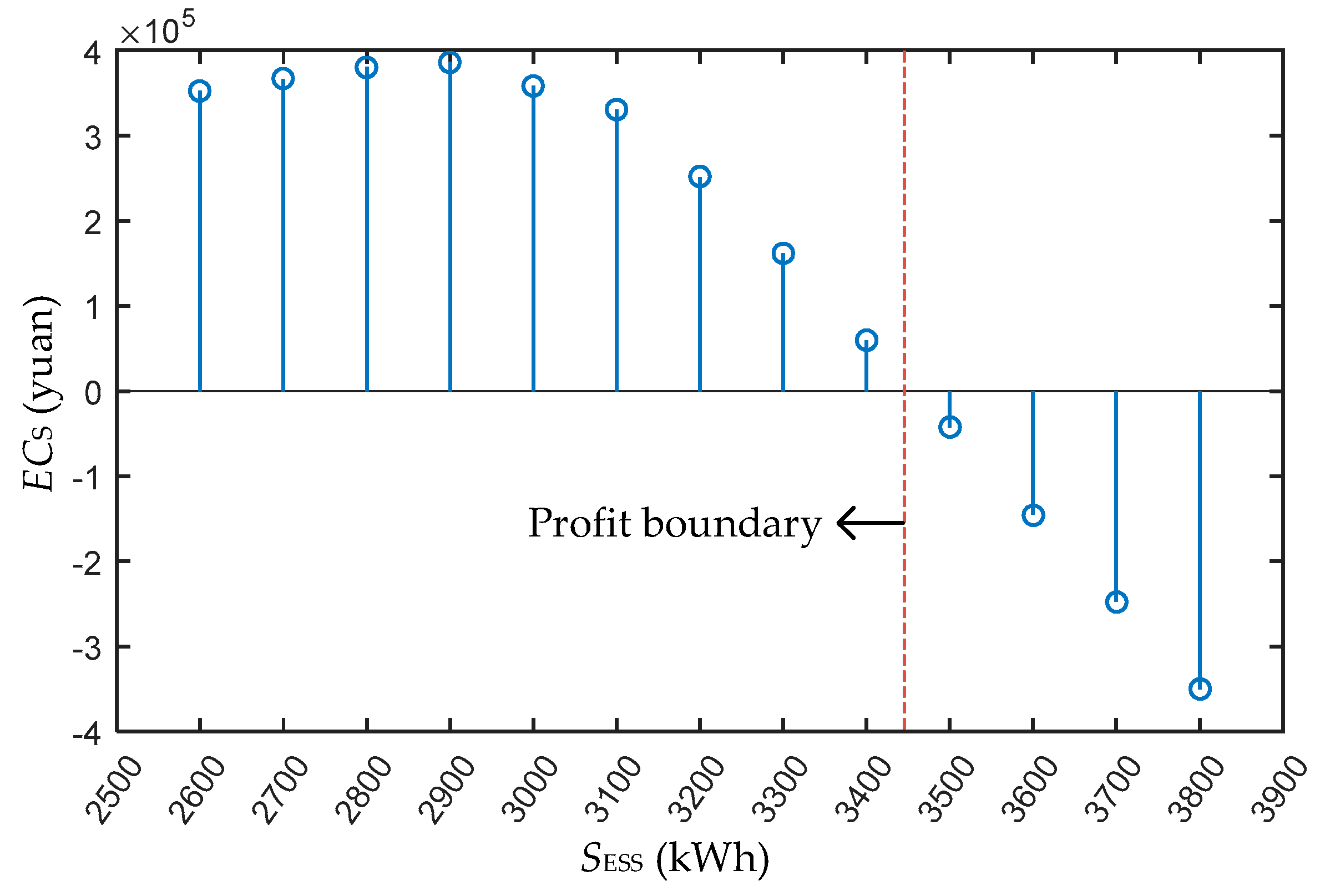
3.2. Profit Boundary of Investment

In order to explore whether there exists a possible profit boundary for a certain capacity of ESS deployment $S_{\mathrm{ESS}}$, extended cases were tested. The criterion $E{C}_{\mathrm{S}}$ with different ESS capacity deployments, i.e., different $S_{\mathrm{ESS}}$ settings, can be calculated and illustrated, as in Figure 5. The length and direction of the blue pointer represents the size and positivity or negativity of the criterion, respectively. When $S_{\mathrm{ESS}}$ is less than 3400 kWh, $E{C}_{\mathrm{S}}$ > 0, indicating that the investment program is economically feasible. When the capacity exceeds 3500 kWh, $E{C}_{\mathrm{S}}$ < 0, indicating it is not worth investing in because the cost is larger than its benefit. When $S_{\mathrm{ESS}}$ is increased from 3400 to 3500 kWh, $E{C}_{\mathrm{S}}$ slowly changes from positive to negative. Additionally, the capacity of the profit horizon can be found between 3400 and 3500 kWh. That is, investment is profitable before the profit boundary and unprofitable after it. Moreover, it can be easily observed that the economic attractiveness or resistance for an ESS investor reflected in the value of $E{C}_{\mathrm{S}}$ with different $S_{\mathrm{ESS}}$. Specifically, the optimal economic attractiveness and sizing of ESS is about 2900 kWh. As with larger ESS deployments, higher investment costs will be paid while less profit could be obtained, in which the profit margin would shrink to zero or even cause a loss.

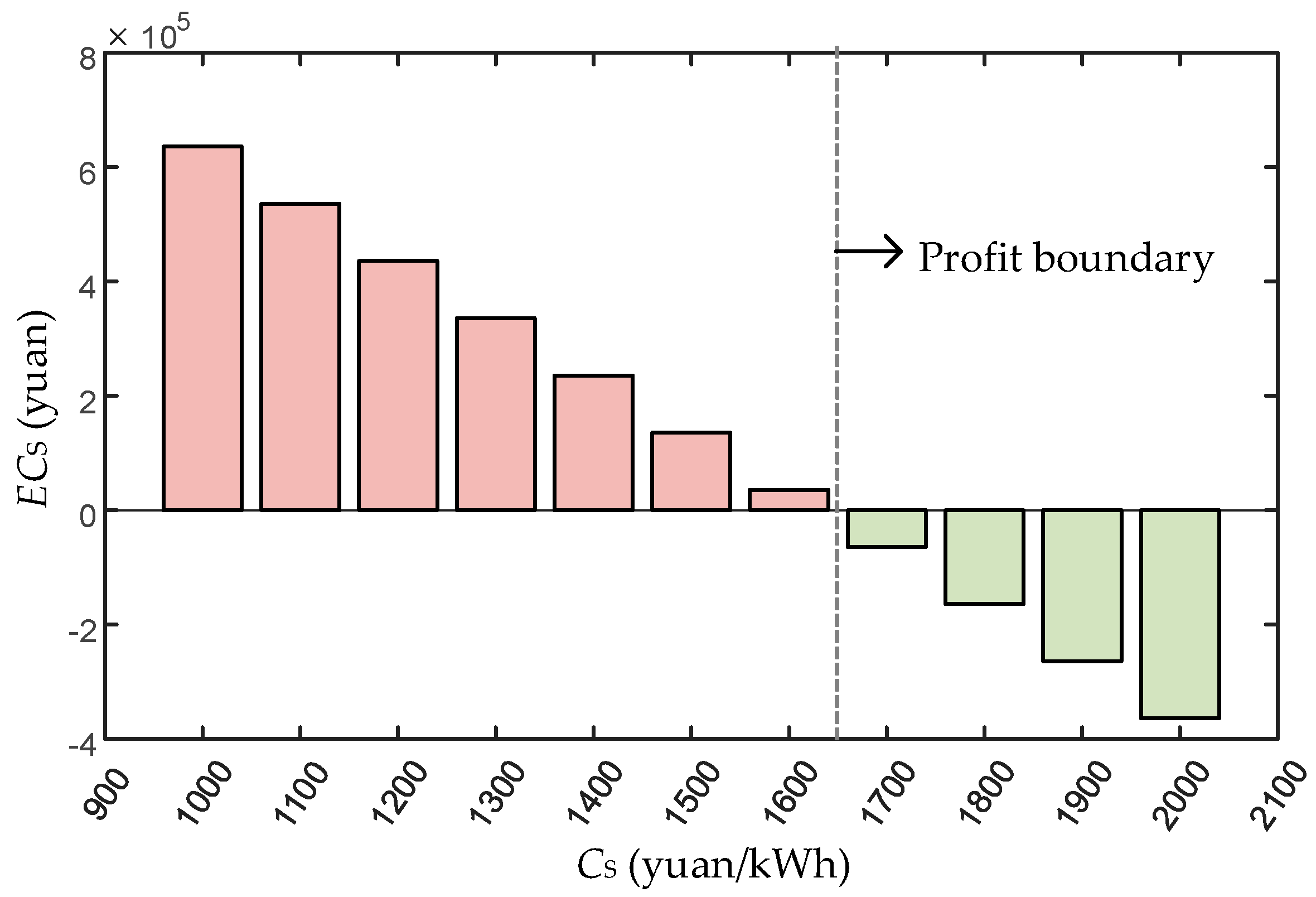
3.3. Sensitivity Analysis of Price

In order to investigate the impact of key parameters on ESS investment feasibility, extended simulation scenarios and results are given in

Table 2. Simulation results and verification with different parameter settings.

Scenario #	SESS (kWh)	CS (yuan/kWh)	Electricity Price Type	Is There Government Subsidy?	ECS (yuan)	Is Energy Storage Economically Needed?
1	3400	1500	#1	Yes	59,819.42	Yes
2	3500	1500	#1	Yes	−42,646.24	No
3	3500	1200	#1	Yes	1,005,303.40	Yes
4	4800	1200	#1	Yes	64,906.61	Yes
5	4900	1200	#1	Yes	−7081.25	No
6	1000	1500	#1	Yes	135,856.94	Yes
7	1000	1500	#2	Yes	180,012.00	Yes
8	1000	1500	#3	Yes	1,557,148.99	Yes
9	1000	1500	#1	No	−620,143.05	No

, while Figure 6 indicates the price information of different types. Column 2 of Table 2 is the capacity of ESS. Column 3 represents the unit price of ESS, while column 4 indicates the type of electricity price. Column 5 indicates whether there is government subsidy. Changes in the above key parameters will have a great impact on the economic efficiency of ESS investments. Then, column 6 indicates the corresponding value of EC in different scenarios. In addition, the final output—“whether energy storage is economically needed to be integrated into the particular microgrid” in each scenario by giving “yes” or “no”—is shown in column 7.

As indicated in Table 2, when $S_{\mathrm{ESS}}$ is set as 3400 kWh in scenario #1, $E{C}_{\mathrm{S}}$ = 59,819.42 yuan, which satisfies $E{C}_{\mathrm{S}}$ > 0. It indicates ESS is economically needed in this scenario. Moreover, the value of $E{C}_{\mathrm{S}}$ represents the profit difference, which can also reflect the economic attractiveness (when $E{C}_{\mathrm{S}}$ > 0) or economic resistance (when $E{C}_{\mathrm{S}}$ < 0) for ESS investment in the microgrid. Besides, the larger $\left|E{C}_{\mathrm{S}}\right|$ is, the larger the economic attractiveness or resistance. Such as $\left|E{C}_{\mathrm{S}}\right|$ in scenario #3 is much larger than that in scenario #4, which indicates ESS is more economically feasible to be planned in the microgrid with its given parameters; while $\left|E{C}_{\mathrm{S}}\right|$ in scenario #2 is much larger than that in scenario #5, which indicates more economic penalties would be incurred with the ESS’s integration. Additionally, both scenario #2 and #5 are unprofitable.

In addition to the impact of the capacity on the economic feasibility of ESS deployments, the static investment economic criterion could also be affected by the unit price of initial investment and the electricity price. Let scenario #2 be the base scenario for analyzing unit price impacts. By comparing scenario #2 and #3, it indicates C_S is reduced by 300 yuan/kWh, and deploying ESS of 3500 kWh will turn from loss to profit. Moreover, the profit boundary horizon of ESS deployments in the microgrid varies by changing the unit price. For example, according to the results of scenario #1 and #2, the profit boundary of ESS sizing locates in [3400, 3500] kWh, while it is [4800, 4900] kWh from scenario #4 and #5. Different C_S contributes to that condition. Similarly, compared with type #1 price in scenario #6, the value of $E{C}_{\mathrm{S}}$ is changed from 135,856.94 yuan to 180,012.00 yuan with type #2 price in scenario #7. In addition to the common peak and valley TOU price (type #1, #2), a spot price (type #3), for example, is simulated in scenario #8. Compared with scenario #6 and #7, the result (1,557,148.99 yuan) of $E{C}_{\mathrm{S}}$ indicates that the introduction of ESS may gain higher benefits in the spot market if the operator can accurately predict the electricity price. Government subsidies are also an important factor affecting $E{C}_{\mathrm{S}}$. Comparing scenario #6 and scenario #9, it can be seen that when there is no government subsidy, the ESS will not be profitable.

Furthermore, Figure 7 shows the additional analysis for unit price of initial investment. The horizontal axis represents the change in price. Additionally, the red and green columns are the size of $E{C}_{\mathrm{S}}$, which indicates profit and loss. Among the costs of ESS, initial investment costs account for the majority. Using the parameters of the base case, the profit boundary for the investment unit price has been explored. That is, investment in ESS with an investment unit price of more than 1700 yuan is not profitable. On the contrary, if the unit price of investment is reduced to less than 1600 yuan, the ESS can achieve profitability. In other words, there is a border price between 1600 and 1700 yuan. Thus, whether the ESS can be profitable depends largely on whether the unit price can be reduced to the border price. This is the key point for the development of ESS.

3.4. Criterion for Long-Term Investment Project

The static investment economic criterion is more suitable for a shorter life cycle. If the life cycle is longer, or considering long-term investment projects, the time value of currency cannot be ignored. Therefore, the dynamic investment economic criterion, which is for pre-defined project cycles, is proposed to judge the economic feasibility of ESS investment. Let $c_{\mathrm{s}}$ = 1000 yuan/kWh. Assume that the predefined project cycle happens to be a life cycle of the energy storage device; Figure 8 shows the difference with changing of capacity between the two criteria. It can be observed that $E{C}_{\mathrm{S}}$ is better than $E{C}_{\mathrm{D}}$ and the profit boundary indicated by $E{C}_{\mathrm{S}}$ appears later than is indicated by $E{C}_{\mathrm{D}}$ with the increasing of ESS capacity. In detail, the values of $E{C}_{\mathrm{S}}$ are always larger than that of $E{C}_{\mathrm{D}}$ no matter what the capacity is. Additionally, the border capacities of $E{C}_{\mathrm{S}}$ and $E{C}_{\mathrm{D}}$ are respectively in the [6, 7] MWh and [3, 4] MWh. This is because $E{C}_{\mathrm{D}}$ calculates the depreciation of the currency. That is to say, the result of $E{C}_{\mathrm{D}}$ is more realistic, especially in the case of a long life cycle. The shorter the life cycle, the closer the values of the two criteria are. ESS investors can choose a criterion to help them make decisions based on their needs.

4. Conclusions

In this paper, two economic criteria were proposed to judge the economic feasibility of integrating ESS into a microgrid. The conclusions obtained in the case study are as follows:

(1) Nowadays, compared with the gains through peak-valley price differences, the investment cost of energy storage is higher. When the investment cost is reduced beyond a certain value (i.e., the profit boundary), the investment in the ESS can be profitable. Furthermore, implementing subsidy policies and developing the electricity market are also ways to increase energy storage earnings.

(2) The profit boundary for ESS capacity due to the size of the microgrid can be found by the proposed economic criteria which can be quickly calculated to evaluate the economic feasibility of an investment program. It can help determine the reasonable capacity of ESS integration and it is affected by factors such as unit price and electricity price.

(3) The static investment economic criterion can be used to judge the economic feasibility of integrating ESS in the short term. It is more suitable to use the dynamic investment economic criterion in a long project cycle.

(4) The two economic criteria can guide the investment behavior of ESS in grid-connected microgrids. Additionally, the method proposed in this paper can make a complete cost-benefit analysis and evaluation of investment plans.

For future work, the more operating modes and the more application scenarios of ESS, such as participating in ancillary services, smoothing renewable energy, and comprehensive utilization, will be considered in the subsequent research.

References

1. Zhang, W.; Qiu, M.; Lai, X. Application of energy storage technologies in power grids. Power Syst. Technol. 2008, 32, 1–9. [Google Scholar]
2. Zia, M.F.; Elbouchikhi, E.; Benbouzid, M. Microgrids energy management systems: A critical review on methods, solutions, and prospects. Appl. Energy 2018, 222, 1033–1055. [Google Scholar] [CrossRef]
3. Khiareddine, A.; Salah, C.B.; Rekioua, D.; Mimouni, M.F. Sizing methodology for hybrid photovoltaic/wind/hydrogen/battery integrated to energy management strategy for pumping system. Energy 2018, 153, 743–762. [Google Scholar] [CrossRef]
4. Luthander, R.; Widén, J.; Munkhammar, J.; Lingfors, D. Self-consumption enhancement and peak shaving of residential photovoltaics using storage and curtailment. Energy 2016, 112, 221–231. [Google Scholar] [CrossRef]
5. Liu, J.; Yang, D.; Yao, W.; Fang, R.; Zhao, H.; Wang, B. PV-based virtual synchronous generator with variable inertia to enhance power system transient stability utilizing the energy storage system. Prot. Control Mod. Power Syst. 2017, 2, 39. [Google Scholar] [CrossRef]
6. Bahramirad, S.; Reder, W.; Khodaei, A. Reliability-constrained optimal sizing of energy storage system in a microgrid. IEEE Trans. Smart Grid 2012, 3, 2056–2062. [Google Scholar] [CrossRef]
7. Karami, H.; Sanjari, M.J.; Tavakoli, A.; Gharehpetian, G.B. Optimal scheduling of residential energy system including combined heat and power system and storage device. Electr. Mach. Power Syst. 2013, 41, 765–781. [Google Scholar] [CrossRef]
8. Feng, L.; Zhang, J.; Li, G.; Zhang, B. Cost reduction of a hybrid energy storage system considering correlation between wind and PV power. Prot. Control Mod. Power Syst. 2016, 1, 11. [Google Scholar] [CrossRef]
9. Xiang, Y.; Han, W.; Zhang, J.; Liu, J.; Liu, Y. Optimal sizing of energy storage system in active distribution networks using Fourier-Legendre series based state of energy function. IEEE Trans. Power Syst. 2017, 33, 2313–2315. [Google Scholar] [CrossRef]
10. Tewari, S.; Mohan, N. Value of NAS energy storage toward integrating wind: Results from the wind to battery project. IEEE Trans. Power Syst. 2013, 28, 532–541. [Google Scholar] [CrossRef]
11. Xiang, Y.; Wei, Z.N.; Sun, G.Q.; Sun, Y.H.; Shen, H.P. Life cycle cost based optimal configuration of battery energy storage system in distribution network. Power Syst. Technol. 2015, 39, 264–270. [Google Scholar]
12. Wu, W.; Hu, Z.; Song, Y. Optimal sizing of energy storage system for wind farms combining stochastic programming and sequential Monte Carlo simulation. Power Syst. Technol. 2018, 42, 1055–1062. [Google Scholar]
13. Bendato, I.; Bonfiglio, A.; Brignone, M.; Delfino, F.; Pampararo, F.; Procopio, R.; Rossi, M. Design criteria for the optimal sizing of integrated photovoltaic-storage systems. Energy 2018, 149, 505–515. [Google Scholar] [CrossRef]
14. Zsiborács, H.; Hegedűsné Baranyai, N.; Vincze, A.; Háber, I.; Pintér, G. Economic and technical aspects of flexible storage photovoltaic systems in Europe. Energies 2018, 11, 1445. [Google Scholar] [CrossRef]
15. Home-Ortiz, J.M.; Pourakbari-Kasmaei, M.; Lehtonen, M.; Mantovani, J.R. Optimal location-allocation of storage devices and renewable-based DG in distribution systems. Electr. Power Syst. Res. 2019, 172, 11–21. [Google Scholar] [CrossRef]
16. Liu, Z.; Chen, Y.; Zhuo, R.; Jia, H. Energy storage capacity optimization for autonomy microgrid considering CHP and EV scheduling. Appl. Energy 2017, 210, 1113–1125. [Google Scholar] [CrossRef]
17. Atia, R.; Yamada, N. Distributed renewable generation and storage system sizing based on smart dispatch of microgrids. Energies 2016, 9, 176. [Google Scholar] [CrossRef]
18. Atia, R.; Yamada, N. Sizing and Analysis of renewable energy and battery systems in residential microgrids. IEEE Trans. Smart Grid 2016, 7, 1204–1213. [Google Scholar] [CrossRef]
19. Chen, S.X.; Gooi, H.B.; Wang, M.Q. Sizing of energy storage for microgrids. IEEE Trans. Smart Grid 2012, 3, 142–151. [Google Scholar] [CrossRef]
20. Xiao, H.; Pei, W.; Yang, Y.; Qi, Z.P.; Kong, L. Energy storage capacity optimization for microgrid considering battery life and economic operation. High Volt. Eng. 2015, 41, 3256–3265. [Google Scholar]
21. Lorestani, A.; Gharehpetian, G.B.; Nazari, M.H. Optimal sizing and techno-economic analysis of energy- and costefficient standalone multi-carrier microgrid. Energy 2019, 178, 751–764. [Google Scholar] [CrossRef]
22. Alsaidan, I.; Alanazi, A.; Gao, W.; Wu, H.; Khodaei, A. State-Of-The-Art in microgrid-integrated distributed energy storage sizing. Energies 2017, 10, 1421. [Google Scholar] [CrossRef]
23. Xiang, Y.; Liu, Y.; Liu, J.; Liu, Y.; Zuo, K. An economic criterion for distributed renewable generation planning. Electr. Power Compon. Syst. 2017, 45, 1298–1304. [Google Scholar] [CrossRef]
24. Sideratos, G.; Hatziargyriou, N. An advanced statistical method for wind power forecasting. IEEE Trans. Power Syst. 2007, 22, 258–265. [Google Scholar] [CrossRef]
25. Tao, C.; Shanxu, D.; Changsong, C. Forecasting power output for grid-connected photovoltaic power system without using solar radiation measurement. In Proceedings of the 2nd International Symposium on Power Electronics for Distributed Generation Systems, Hefei, China, 16–18 June 2010. [Google Scholar]
26. Balci, H.; Valenzuela, J. Scheduling electric power generations using particle swarm optimization combined with the Lagrangian relaxation method. Int. J. Appl. Math. Comput. Sci. 2004, 14, 411–421. [Google Scholar]
27. Jiang, Y.C.; Wang, Z.G.; Yang, C.Y.; Li, M.; Zhang, J.P. Multi-objective optimization strategy of controllable load in microgrid. Power Syst. Technol. 2013, 37, 2875–2880. [Google Scholar]
28. Luo, Y.; Liu, M. Research on environmental and economic dispatch for isolated microgrid system taken risk reserve constraints into account. Power Syst. Technol. 2013, 37, 2705–2711. [Google Scholar]
29. Shen, Y.; Hu, B.; Xie, K.; Xiang, B.; Wan, L. Optimal economic operation of isolated microgrid considering battery life loss. Power Syst. Technol. 2014, 38, 2371–2378. [Google Scholar]
30. Rydh, C.J.; Sandén, B.A. Energy analysis of batteries in photovoltaic systems. Part I: Performance and energy requirements. Energy Convers. Manag. 2005, 46, 1957–1979. [Google Scholar] [CrossRef]
31. Yan, G.; Liu, D.; Li, J.; Mu, G. A cost accounting method of the Li-ion battery energy storage system for frequency regulation considering the effect of life degradation. Prot. Control Mod. Power Syst. 2018, 3, 4. [Google Scholar] [CrossRef]
32. Tran, D.; Khambadkone, A.M. Energy management for lifetime extension of energy storage system in micro-grid applications. IEEE Trans. Smart Grid 2013, 4, 1289–1296. [Google Scholar] [CrossRef]
Figure 1. Typical correlation profile of the maximum cycles and depth of the discharging (DOD).
Energies 12 02312 g001
Figure 2. Typical load, PV, and WT profiles.
Energies 12 02312 g002
Figure 3. ESS-state of charge (SOC) result in the base case.
Energies 12 02312 g003
Figure 4. ESS charging and discharging results in the base case.
Energies 12 02312 g004
Figure 5. ECS (static investment economic criterion) values with different ESS capacity deployments.
Energies 12 02312 g005
Figure 6. Electricity price of different types (type #1–3).
Energies 12 02312 g006
Figure 7. ECS values with different unit prices of initial investment.
Energies 12 02312 g007
Figure 8. Values of two criteria with different ESS capacity deployments.
Energies 12 02312 g008