OpenHPL for Modelling the Trollheim Hydropower Plant


Department of Electrical engineering, Information Technology and Cybernetics, University of Southeastern Norway, 3901 Porsgrunn, Norway
*
Author to whom correspondence should be addressed.
Energies 2019, 12(12), 2303; https://doi.org/10.3390/en12122303
Submission received: 23 April 2019
/
Revised: 24 May 2019
/
Accepted: 12 June 2019
/
Published: 17 June 2019
Abstract
:An increase of tightly integrated, renewable energy sources with highly varying production leads to a greater need for flexible hydropower plants to “balance” the intermittent production from these sources. From a systems perspective, the intermittency aspect constitutes a disturbance, while the tight integration leads to a multivariable systems, both of which causes increased challenges for good control. This instigates the need for a model based analysis and synthesis tool which can describe dynamic phenomena, supports multiphysics problems, and allows for immediate use in advanced control analysis and design. Previously, an open source Hydro Power Library (OpenHPL) have been developed within the multiphysics Modelica eco-system which satisfies the above requirements: OpenHPL contains a set of model units relevant for hydropower systems, as well as examples of tools for analysis of these models for control purposes. Thus far, OpenHPL has been validated by comparison against other simulation tools. However, a real test of OpenHPL is to use it to describe a real hydropower plant using minimal plant information, to tune model parameters against experimental data, and to validate the model. As a case study, experimental data from the Trollheim hydropower plant in Norway have been made available, and used to test OpenHPL. By flow sheeting a hydropower model in OpenModelica using OpenHPL, the model can be simulated from within a script language (Python via the OMPython API, Julia via the OMJulia API) and further analyzed using analysis tools in the script language. Based on default model parameter suggestions from OpenHPL, least squares model fitting was carried out in Python, and the model was validated with good model fit. Important parts of the modelling phase were the development of a new friction model for the Francis turbine, and iterations on the description of the turbine outlet geometry. The results are complemented with a discussion of possible uses of the model.
1. Introduction
1.1. Background
A transition towards more renewable, and tightly integrated energy sources is currently happening in Europe and all over the world. This situation leads to increase in the use of flexible hydropower plants to compensate the highly changing production from intermittent energy sources such as wind and solar irradiation. Intermittency implies disturbance from a control systems perspective, and tight integration implies multivariate behavior. This instigates the need for new, modern multiphysics simulation tools with support for hydropower systems, which at the same time can be tightly integrated with tools for advanced control analysis and synthesis. A modern trend is towards open source tools which can be freely used in education, and which allows for user participation in the further development. High head hydropower plants are particularly important for balancing intermittent energy sources, and also play an important role in Norway.
A general research question is then: how should an open source simulation tool for hydropower systems be designed? A partial answer lies in the previous development of a hydropower library OpenHPL within the multiphysics modelling language Modelica, and the development of analysis tools in, e.g., Python or Julia, which can interact with the Modelica code via APIs OMPython and OMJulia in the free tool OpenModelica. Because Modelica is a multiphysics language, a waterway model based on OpenHPL can be directly connected to a model of the electric grid (based on electric libraries), and to any other system modelled in Modelica—as long as the interfaces are compatible.
In this paper, we consider the more specific research question: how suitable is OpenHPL for describing a real hydropower plant, and how can model parameters be tuned to fit experimental data? To answer this question, experimental data from the Trollheim hydropower plant in Norway have been made available.
1.2. Previous Work
In general, waterway dynamics of high head hydropower systems can be represented by a model of water flow in pipes. Hence, mass and momentum balances are normally used for modelling of the waterway units. Depending on the desired level of accuracy, models of the waterway unit can be described by ordinary differential equations (ODEs) in cases with incompressible water and inelastic walls. Partial differential equations (PDEs) appear for the more realistic cases with elastic walls and compressible water; various principles of solving the resulting hyperbolic PDEs are used. Model of turbine units can be based on using the Euler turbine equation in the case of a mechanistic model, or based on look-up tables (static characteristic curves for specific turbines)—for an empirical model. Some work on models for these units of the hydropower systems has already been presented in the literature [1,2,3,4]. Applications of hydropower models have also been published in [5,6,7]. Various examples of software tools for hydropower modelling also exist, and a basic overview of some of them has been given in [8].
One of these hydropower modelling tools is LVTrans [9] which is based on LabView [10] for transient simulations of hydropower plants [11]. LVTrans uses a MOC (Method of Characteristics) solver for simulation of PDEs. Turbine units in LVTrans are described by physical models that only need the turbine nominal operating values and do not need look-up tables for simulation.
Another tool, TOPSYS, a combined effort of Wuhan University and Uppsala University, is based on Visual C++ and provides models for various components of hydropower plants [6,12]. This software allows for simulation of elastic conduits with compressible water described by PDEs. Turbine models in TOPSYS are based on look-up tables, which requires fitting a model to experimental data or use of static characteristic curves for specific turbines.
SIMSEN [13] is a simulation tool for the analysis of electrical power networks, adjustable speed drives and hydraulic systems, developed and used at École Polytechnique Fédérale de Lausanne [14]. This software uses analogue models (RLC components) for modelling hydraulic elements. Turbine units in SIMSEN are also modelled based on look-up tables.
The commercial Modelica Hydro Power Library [15] from Modelon [16] provides a framework for modelling and simulating hydropower plant operations in a commercial Modelica-based modelling and simulation environment—Dymola [17,18,19]. This Modelica library uses staggered grid for discretization and simulation of PDEs. Description of the turbines is based on look-up tables for this Hydro Power Library.
Among these modelling and simulation tools for hydropower systems, only LVTrans is currently open-source software and freely available. However, LVTrans is based on and requires the commercial tool LabView, and is thus not truly openly accessible. In addition, LVTrans is used only for transient simulations of hydropower plants and is not the multiphysics tool. The Modelica Hydro Power Library from Modelon as well as SIMSEN support multiphysics systems.
Our work on modelling the waterway and the Francis turbine for high head hydropower systems using the multiphysics tool OpenModelica [20], has been reported in [21,22,23]. Unit models have been developed for our in-house open-source Modelica [24] library—OpenHPL (Open Hydro Power Library is developed by the first author within his PhD study).
A Python API named OMPython [25] for OpenModelica already exists which provides possibilities for controlling simulations of the OpenModelica models via Python [26]. Python, in turn, gives much broader possibilities for plotting, analysis, and optimization compared to what is possible in OpenModelica (e.g., using Python packages matplotlib, numpy, scipy, etc.) [27,28].
1.3. Overview of Paper
In this paper, the main contribution is testing the suitability of OpenHPL by building a model of a real hydropower system (Trollheim hydropower plant), fitting model parameters based on experimental data from the plant, and validating the model. Particular emphasis is put into describing the model geometry of the turbine outlet. Moreover, the turbine design algorithm developed in [23] is improved in this study with an analytical expression for the turbine loss coefficients. Both of these contributions try to answer the particular research question: “how suitable is OpenHPL for describing a real hydropower plant with minimal prior information, and how can model parameters be tuned to fit experimental data?”.
The paper is structured as follows: Section 2 provides a system description of the Trollheim hydropower plant and describes the experimental conditions. Section 3 gives an overview of hydropower modelling with the developed OpenHPL library and presents model cases of the Trollheim hydropower plant. Simulation results of the hydropower models that are tuned and fitted to real measured data are presented in Section 4. Finally, the discussion is given in Section 5 and the final section provides the conclusions.
2. System Description
2.1. Geometry Data
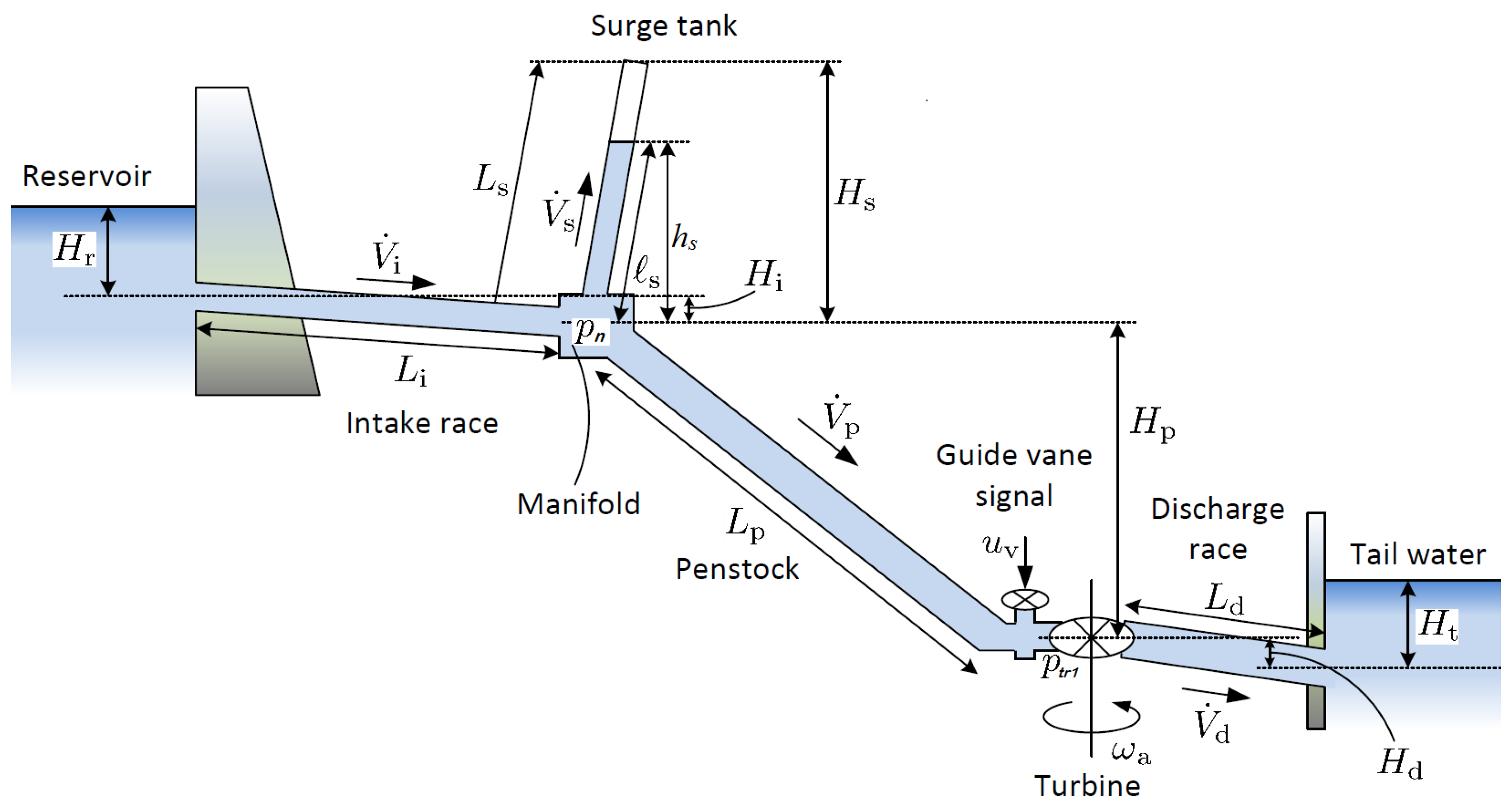
High head hydropower plants typically collect and store water in reservoirs in mountains, with tunnels leading the relatively small flow of water down a considerable height difference to the aggregated turbine and generator. The electricity produced by the generator is then transferred through power lines to consumers. More detailed description of the hydropower system has been presented in our previous work [21,22]. A typical structure of a high head hydropower plant is depicted in Figure 1 [21].
In this paper, the Trollheim hydropower plant [29] operated by Statkraft is used as a case study. The geometry data of this hydropower plant are provided in Table 1 and Table 2. It should be noted that the structure of the Trollheim plant is similar to that presented in Figure 1, but all of the conduits (penstock, intake and discharge races) have more complex structures. These units consist of series of connected conduits with different geometry (length, slope, etc.), e.g., the intake race is divided into three parts: intake race #1, #2 and #3.
From Table 1, it should be clarified that the height difference for the reservoir corresponds to the water level in this water storage. In addition, a negative height difference represents a rising slope of the conduit, e.g., in the intake race #2 and discharge race #2: this negative height difference means that the inlet to the conduit has lower altitude in respect to sea level than the outlet.
It should also be noted that not all of the waterway units (e.g., intake or discharge races) are circular conduits. However, Table 1 presents diameter values for each waterway unit, which means that the circular conduit is used in our library for all unit models and the given diameter provides the same cross sectional area as the conduits have in reality.
2.2. Experimental Data
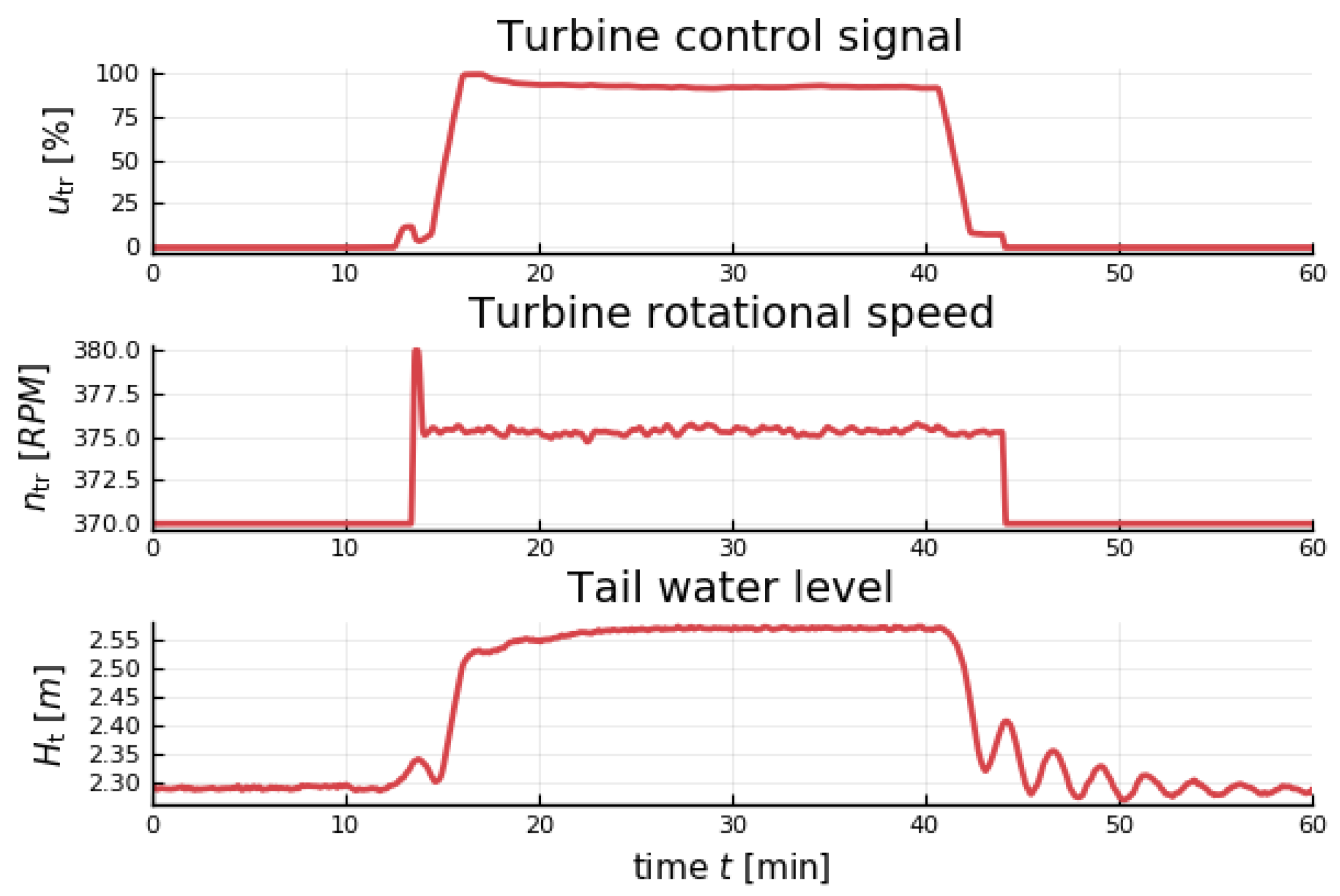
The experiment on the Trollheim hydropower plant has been done using the HydroCord monitoring system, developed by [30]. The experimental measurements are taken within a one-hour window when the hydropower plant was run from zero to full load and after some time back from full to zero load. The experimental data consist of measurements with a sampling time of one second. All measured variables are listed in Table 3, and their values are available in Github [31]. Among these measured quantities are the variables that provide input information for our models. Other quantities belong to the models’ outputs and can then be used for model fitting and validation. It should be mentioned that not all variables listed as “model input” in Table 3 are proper inputs/causes for the system. The proper input is the turbine control signal, while turbine rotational speed and tail water level are responses of this proper input. However, we have not included models of the rotational speed or tail water level, so, from a model fitting point of view, we need to use “model input” to simulate the system.
The variation in the water level in the reservoir is also provided, but these changes are so small that we neglect them here and assume the reservoir water level to be constant.
For better understanding of the experiment, the experimental measurement of the signals that belong to model inputs are shown in Figure 2. The output measurements are presented in Section 4, where comparisons of these measurements and model outputs are shown. It is seen from Figure 2 that, after approximately 12 min of fully closed turbine guide vanes, the control signal increases to 100% in approximately 6 min. Then, the control signal slightly decreases to a nominal value of approximately 93% and the hydropower plant runs with the nominal load for 25 min. After approximately 40 min, the control signal closes the turbine guide vane openings over 3 min, and the remaining time these guide vanes stay closed.
Figure 2 shows that, even with closed guide vanes (no water flow through the turbine), the rotational speed is still observed and is close to nominal value. This is because the generator is working as an electrical consumer in this regime and rotate the shaft with the turbine runner. This is done in order to make generator synchronization easier when the power plant is turned on full load. The generator starts to produce electricity only when the nominal rotational speed is reached.
3. Hydropower Modelling
In this section, a description of how to model the hydropower system using the OpenHPL is given as well as a presentation of various cases of the Tollheim hydropower plant model for the further comparison with the measurements. As mentioned above, all modelling is done in OpenModelica, which is an open source Modelica-based modelling and simulation environment intended for industrial and academic usage. Modelica in turn is a multi-domain and component-oriented modelling language that is suitable for complex system modelling (some tutorials exist for Modelica [32], and OpenModelica [33]).
3.1. Hydropower Library Overview
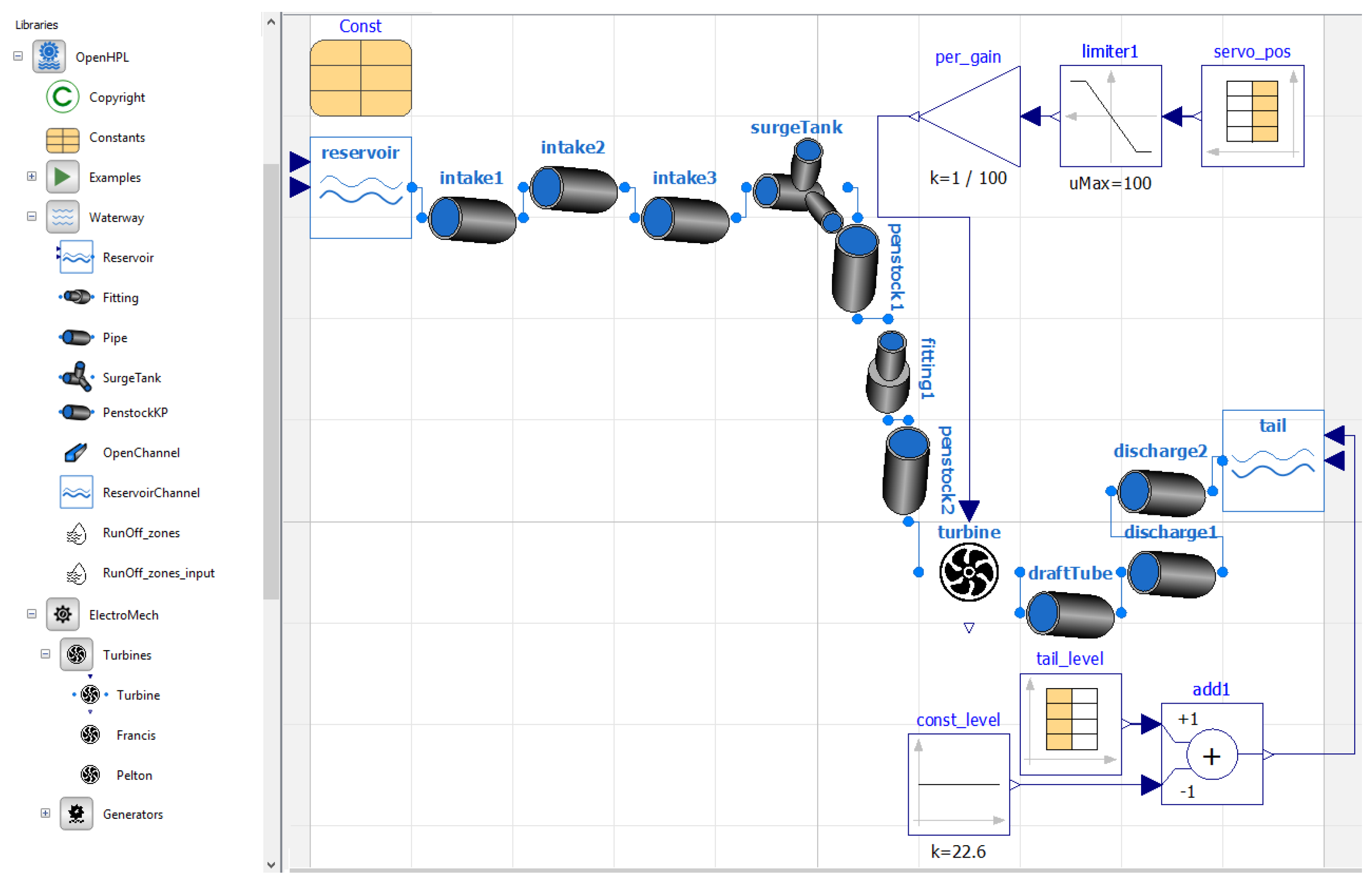
For modelling of the hydropower system, library OpenHPL is used. This is an in-house hydropower library consisting of drag and drop elements that describe different units of the hydropower system such as reservoir, conduits, surge tank, and turbine. These elements can be structured in a flow sheet in the same way as the hydropower plant—see the hydropower structure in Figure 1 and the flow sheet in Figure 3. Then, in this flow sheet, all drag and drop elements can be specified with appropriate geometry of the hydropower plant by double-clicking on the element. Connectors that join each element hold information about the pressure in the connector and mass flow rate that flows through the connector—similar to the connection in an electrical circuit with voltage and current.
In comparison to other hydropower modelling tools presented in Section 1.2, OpenHPL has some advantages, perhaps the foremost being that the library is openly accessible with multiphysics support, and support for analysis. Another OpenHPL benefit is related to the included mechanistic Francis turbine model which makes it possible to simulate systems without detailed turbine characteristics; turbine efficiency charts are rarely openly available.
In the sequel, a more detailed description is given of OpenHPL elements related to the waterway and turbine units of the hydropower system.
3.1.1. Waterway Units
In OpenHPL, different waterway components of the hydropower system, e.g., reservoir, conduits, surge tank, are described by both mass and momentum balances, and could include compressible/incompressible water or elastic/inelastic pipe walls. A more detailed overview of the mathematical models and methods used in this library for the waterway components is given in [21,22]. The Pipe element in the library (see the left panel in Figure 3) represents a simple model of a circular conduit with incompressible water and inelastic pipe. This element might be used to model waterway elements, e.g., the intake race, penstock, and discharge race. In some cases, water compressibility and pipe elasticity should be taken into account for a more detailed model of waterway units exposed to large pressure differences, e.g, the penstock. For these cases, the PenstockKP element is available in our library and represents a detailed model of the circular conduit with either compressible water and inelastic pipe or compressible water and elastic pipe. A well-balanced Kurganova–Petrova, Finite Volume scheme is used to solve the partial differential equations [21]. For this method, the number of discretization segments should be set in the PenstockKP element. All other parameters for this element are similar to the Pipe parameters and geometry listed in Table 1.
There are also available Reservoir and SurgeTank elements that represent simple models for the reservoir and surge tank, respectively. More details of these models are given in [22].
3.1.2. Turbine Unit
The turbine unit can be expressed either with a simple turbine model based on a look-up table (turbine efficiency vs. guide vane opening) or with a detailed mechanistic Francis turbine model. The simple turbine model is described by Equation (1), where the mechanical turbine shaft power is defined as:
Here, gives the turbine hydraulic efficiency that is found from a standard turbine look-up table, and depends on the turbine control signal, . is the pressure drop through the turbine, defined as the difference between inlet and outlet turbine pressures: . The relationship between the turbine volumetric flow rate and the pressure drop is described through a simple valve-like expression as follows:
Here, in Equation (2) is the guide vane “valve capacity” that can be tuned by using the nominal turbine net head (nominal pressure drop) and the nominal turbine flow rate listed in Table 2. is the atmospheric pressure.
Based on Equations (1) and (2), the simple turbine model is implemented in OpenHPL as the Turbine element. Our library also includes a mechanistic Francis turbine model that has been presented and described in detail in [23]. In [23], the mechanistic Francis turbine model is provided together with a design algorithm for all the needed turbine geometry parameters that are used in this model. Input data for the design algorithm are the turbine nominal operational values that can be found in Table 2 of this study. Both the Francis turbine model and the turbine design algorithm are realized in the Francis turbine element in our library. However, the friction coefficients that represent shock, , whirl, , and pipe friction losses, , should also be defined for the Francis turbine model [23]. In previous work, these coefficients were tuned using the least squares method to fit the turbine characteristic (power production vs. turbine flow rate) from the model with the same characteristic from the real turbine. The same principle is used and presented in Section 4.
3.2. Model Presentation
Using OpenHPL, models of different complexity for the Trollheim hydropower plant can be modelled in OpenModelica. An example of such a model for the Trollheim plant is shown in the flow sheet in Figure 3. Here, all components are set with geometry data from Table 1 and Table 2. The input signals of the guide vane opening and the water level in the tail water are used in this model.
Four models will be considered in the sequel; the first of these is based on the flow sheet in Figure 3, while the three others represent minor modifications of this flow sheet:
- The model presented in Figure 3 is implemented using the simple Pipe with incompressible water and inelastic pipe walls for all waterway units. Moreover, a simple turbine model based on the look-up table for turbine efficiency is used here.
- Hydropower model with detailed turbine—using the more detailed Francis turbine model (the Francis element in the library) instead of the simple turbine model based on the look-up table (the Turbine element in the library).
- Hydropower model with detailed penstock—using the more detailed penstock model with compressible water and elastic walls (the PenstockKP element in the library) instead of the simple conduit model (the Pipe element in the library).
- Hydropower model with both detailed turbine and penstock (both previous changes together).
Information about the turbine rotational speed is not needed for the simple turbine model (#1, #3 with the Turbine element), hence the measured turbine rotation is not used as the input in the hydropower model presented in Figure 3 . However, the measured turbine rotation is used in the cases with the more detailed Francis turbine model that needs turbine rotational speed information.
It should also be noted that, currently, our hydropower library does not include a proper model for a draft tube unit [34]. However, Figure 3 shows that the flow sheet of the hydropower model includes a draft tube unit described by the simple Pipe element, similarly to modelling of the intake race, discharge race, etc. This Pipe element is used here as a tuning factor and its geometry and shape does not represent the real draft tube. More information about tuning of this draft tube element is provided in Section 4.
4. Model Fitting and Simulation
4.1. Simulation Overview
All simulations that are presented in Section 4 are done in OpenModelica using Python API OMPython to control the simulations, and handling the results in Python. For plotting in Python, the matplotlib package is used. In order to define model tuning parameters that provide the best model fit with the measured data, optimization package scipy is used. This package provides various algorithms that can be used for curve fitting with the least squares error method. More detailed information about the Python API and its use has been presented in [27,28].
The simulations are performed in the same way that the experiment has been done, using the same control input and sampling time. Here, a number of simulations for different models of the hydropower system are presented. First, tuning of the Francis turbine model parameters is shown. After that, the previously discussed four cases of the hydropower model are simulated and compared with the measured data.
4.2. Friction Coefficients for Francis Turbine Model
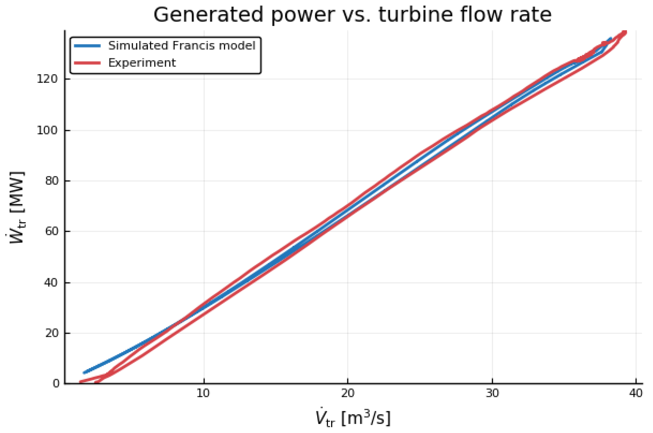
In order to find the turbine loss coefficients: , , and that are used in the mechanistic Francis turbine model, the case of the hydropower model with the detailed mechanistic Francis turbine element is simulated first. The simulations for this model are performed over the time horizon of one hour (the same as in the experiment), but the results within a time interval of approximately 14–44 min is used for comparison with the experimental data. This is due to the need to compare turbine characteristics (the generated power vs. the turbine flow rate) from the model and the experimental data. This characteristic in turn is relevant when the generated power is greater than zero—the turbine runner rotates with the nominal rotational speed (time interval 14–44 min in Figure 2).
4.2.1. Tuning Loss Coefficients
First, the turbine loss coefficients , and have been manually tuned in order to reach an initial fitting of the model simulation results with the measured data from the experiment. In a previous study [23], it was found that typically, , , and . By some manual tuning, here, we found the initial values , and .
Next, we fine tune the loss coefficients using a least squares method in SciPy [35], by using the above initial values as a starting point. From least squares tuning, we find the following loss coefficients: , and . Comparison of the power production vs. turbine flow rate characteristics found from the model simulation with least squares loss coefficients and the experimental data are shown in Figure 4.
It is seen from Figure 4 that the characteristic from the Francis turbine model (blue curve) fits reasonably well the experimental results on the real turbine. There is some deviation between the curves for low flow values close to zero. However, this deviation is not crucial and is caused by the difference between the measured generated power and the turbine shaft power taken from our model simulation. In addition, this deviation confirms the fact that the turbine model does not work well with the low load regimes (low turbine flow rate).
4.2.2. Analytic Expression for Loss Coefficients
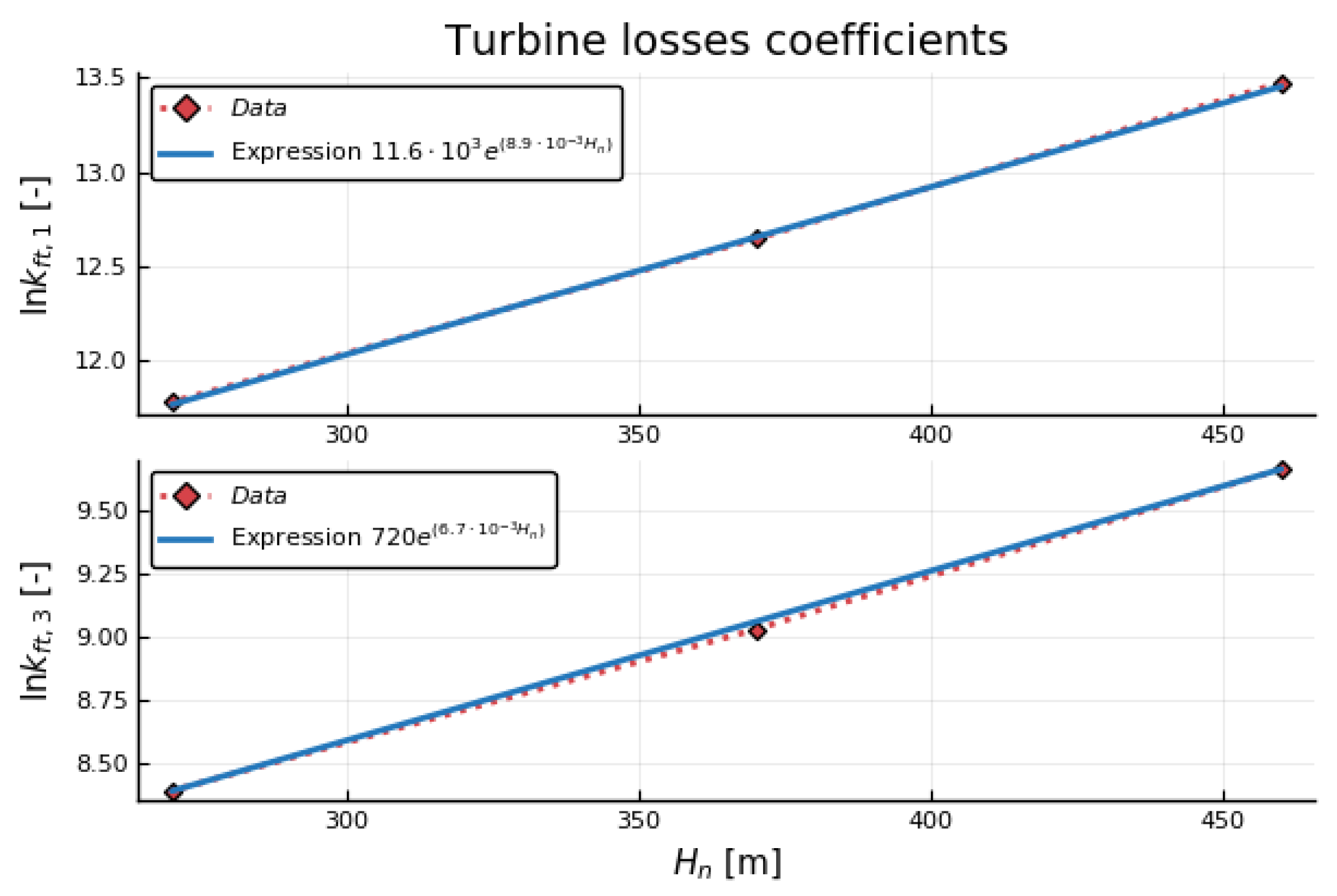
Using the values found from the least squares error method, the turbine design algorithm might be improved with an analytic expression for finding the loss coefficient. This expression can be found using information from two other cases that have been previously described in [23]. Comparing the values for the loss coefficients and the turbine nominal values for all three cases, a relation between the turbine nominal head and two of the coefficients, and , is observed. Loss coefficient, , seems to be negligible and is zero in all three cases. The relation between the turbine nominal head and natural logarithm of the loss coefficients, and , is shown in Figure 5. Here, the three diamond markers in the data represent the value of the loss coefficients for each case of the hydropower system. The figure includes analytic expressions that characterize reasonably well the relations between the turbine nominal head and the loss coefficients. By studying results from model fitting, it has been observed that the logarithm of the turbine loss coefficients appear to be linearly related to the turbine nominal head, Figure 5. We thus propose the following expressions for the turbine loss coefficients:
The exponential expressions for the and turbine loss coefficients represent an important improvement of the turbine design algorithm developed in [23]. With Equations (3) and (4), all the parameters needed for the mechanistic Francis turbine model can be found based on the turbine nominal operation values only.
4.3. Simple Hydropower Model
The model for the complete hydropower system is simulated next in order to see how well the model results fit real experimental data. First, the model that has been shown in Figure 3 is considered with simple turbine and penstock (incompressible water and inelastic walls). The simulations are performed for one hour with the same scenario and sampling time as during the experiment.
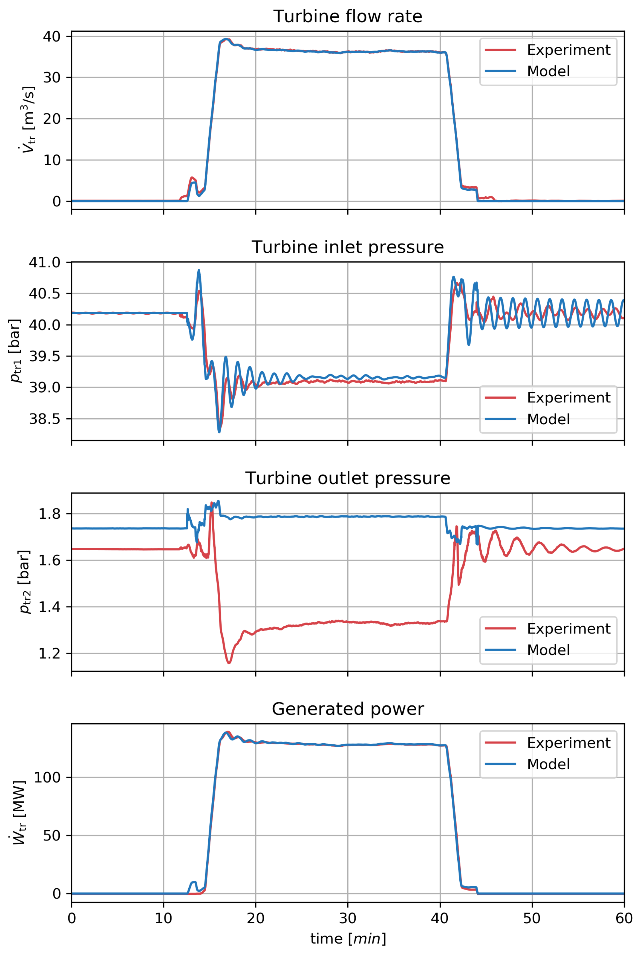
A comparison of the simulation results and the experimental data are shown in Figure 6, where four plots for the turbine flow rate, the turbine inlet and outlet pressures, and the generated power are presented. It should be noted that the model has only been set with the geometry parameters of the Trollheim hydropower plant (Table 1 and Table 2) without any additional tuning. The draft tube is excluded from this simulation to emphasize the importance of including it. It is seen from the figure that the model results fit the experimental data reasonable well, especially for the turbine flow rate and the generated power. The model results for the transient dynamics of the inlet turbine pressure slightly deviate from the measured results (model results with higher oscillation amplitude). For the outlet turbine pressure, the model results show significant deviation in comparison to the experimental measurements. The accuracy of the outlet turbine pressure results is quite important, especially for cavitation studies.
4.3.1. Pipe Roughness: Initial Manual Tuning
In order to improve the model results, the presented hydropower model can be further tuned. An important parameter for controlling friction and damping of oscillations is the pipe surface roughness height, . Thus far, an identical value ( mm) has been used for all pipes. Because the inner pipe surfaces range from that of a rough, drilled tunnel in the intake race, to lined penstocks, this is clearly unrealistic. The ranges of the absolute roughness values for common construction materials are known and could be found from various absolute roughness tables [36].
As mentioned in Section 2, in reality, some of the waterway units have non-circular shape, but in the presented hydropower model all these units are considered as circular conduits. This simplification can also affect the Darcy friction factor because the ratio between roughness height and hydraulic diameter of the conduit, , is used to define the friction factor. For circular conduits, the hydraulic diameter equals simply the diameter of the conduit, however for conduits with other shapes, this hydraulic diameter equals conduit cross sectional area multiplied by four and divided by perimeter of the conduit. Hence, by tuning the roughness parameter, the conduit shape simplification is taken into account.
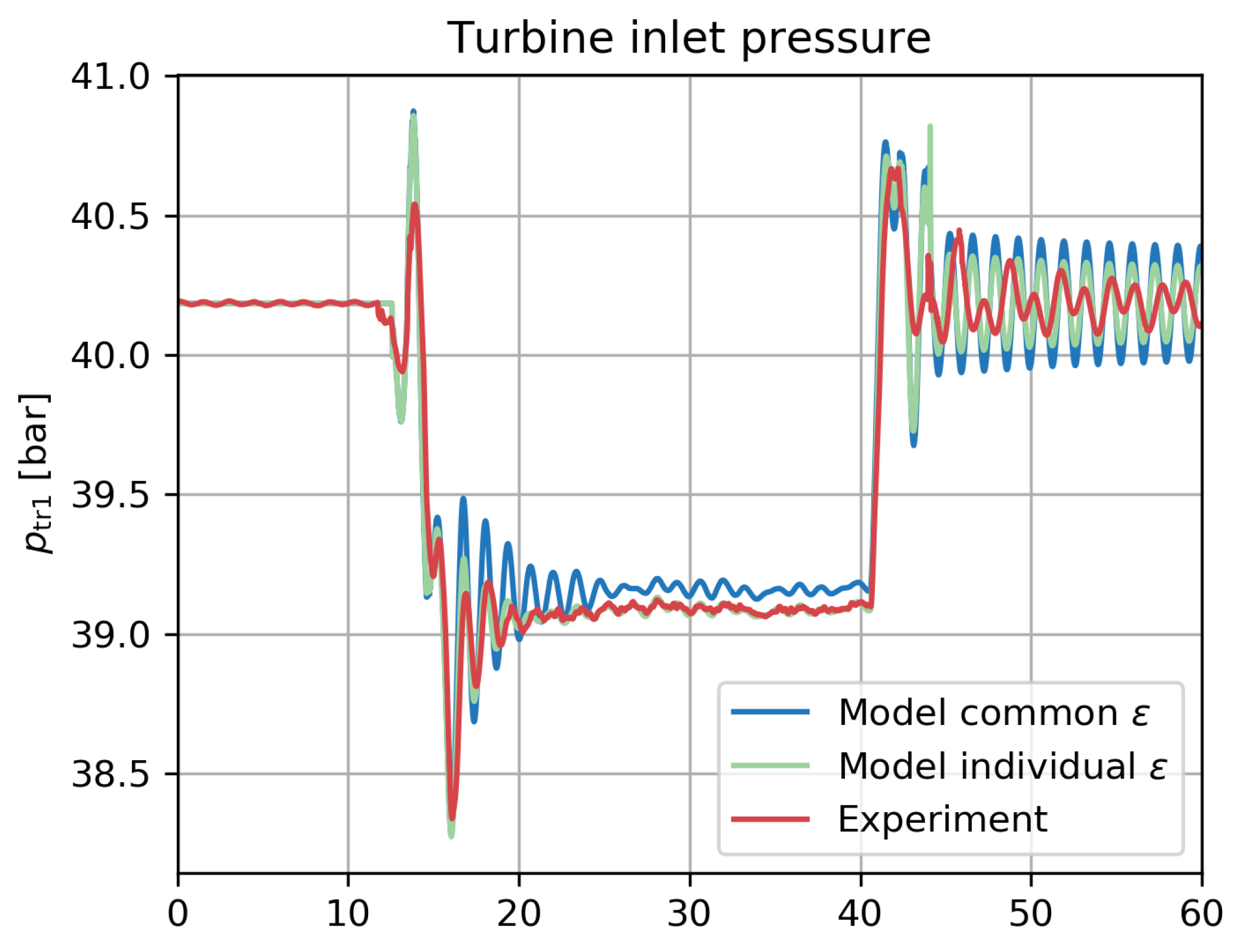
In an initial phase, we manually adjust the roughness heights—the results will later be used as initial guesses in a least squares fitting phase. It is assumed that the intake race roughness is the highest in the waterway, i.e., as a long, rocky tunnel. In the same way, the penstock might have the lowest value for the roughness height, i.e., like a smooth steel pipe. Roughness values for the surge tank and the discharge race might lie somewhere between, i.e., as a smooth concrete pipe. As expected, the manual tuning phase confirms that changes in the roughness heights affect the amplitude of the transient oscillations. A comparison of the inlet turbine pressure from the experimental data, and two models with (i) common roughness height , and (ii) individual roughness heights are shown in Figure 7. For the model with individual roughness values, the roughness height for each waterway unit is set as follows: mm for the intake race #3; mm for the surge tank and intake races #1 and #2; mm for discharge races #1 and #2; and finally penstock #1 and #2 have mm.
Figure 7 shows that the model with individually fitted roughness values for each waterway unit provides better results than the model with fixed (common) roughness for all units. The improvements are visible in the amplitude of the transient oscillation and the results of the model with different roughness deviate less from the experimental data. These improvements are also confirmed by the root mean squared error (RMSE) between the model and experiment inlet pressures. The RMSE is reduced from 0.142 bar for the model with common roughness to 0.104 bar for the model with individual roughness.
4.3.2. Draft Tube Geometry: Initial Manual Tuning
As mentioned above, the draft tube is also used in this hydropower model. However, the geometry of the draft tube situated in the Trollheim hydropower plant is not known in detail, and the simple Pipe element is used in the model. With this pipe element, added geometric parameters are available as tuning parameters for the model. However, the geometry and shape of this Pipe element might not represent the real draft tube.
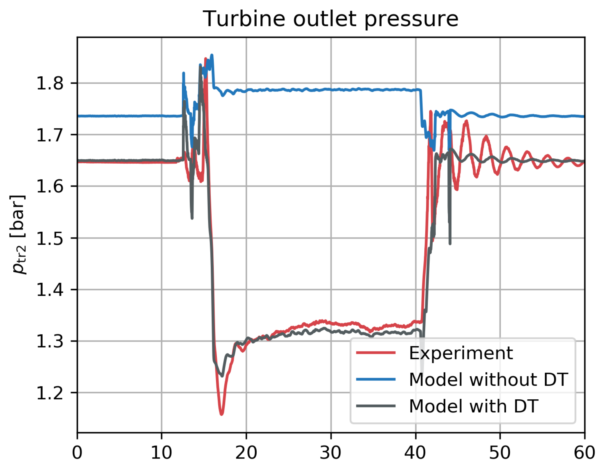
In the previous simulation of the hydropower model, Figure 6, the draft tube element was not been included in the model simulation. With the Pipe element of OpenHPL, it is possible to specify the Pipe element as an expanding circular vertical pipe. Thus, the length, the inlet diameter, the outlet diameter, and the roughness height of this pipe can be tuned. After some manual tuning of the geometry of the draft tube model, it has been observed that this unit significantly affects the turbine outlet pressure dynamic. The simulation results of the hydropower model with and without this draft tube are shown in Figure 8, where the comparison of the turbine outlet pressure from the measurements and the model simulations is provided.
From manual tuning, the draft tube pipe is designed with an expanding diameter from 2.2 m to 3.04 m, 12 m long, and with 0.001 mm roughness height. This pipe geometry deviates from what is expected in a real draft tube: especially the real draft tube shape [34] is much more complicated than the simple vertical expanded pipe used here. Figure 8 shows that the outlet pressure from the model with the simplified draft tube element fits the experimental data much better than the results from the model where the draft tube is not considered. This better fitting is also confirmed by the RMSE of the outlet pressure that has reduced from 0.315 bar for the model without draft tube to 0.038 bar for the model with draft tube.
4.3.3. Pipe Roughness and Draft Tube Geometry: Least Squares Tuning
Starting with the initial parameter guesses from Section 4.3.1 and Section 4.3.2, the least squares method is used to fine tune the model parameters. The results of the simple hydropower model with the parameters tuned by the least squares method are shown in Figure 9, where the four plots: the turbine flow rate, the turbine inlet and outlet pressures, and the generated power are presented. The tuning parameters found with the least squares error method are given in Table 4 and Table 5 for the roughness heights and the draft tube geometry, respectively.
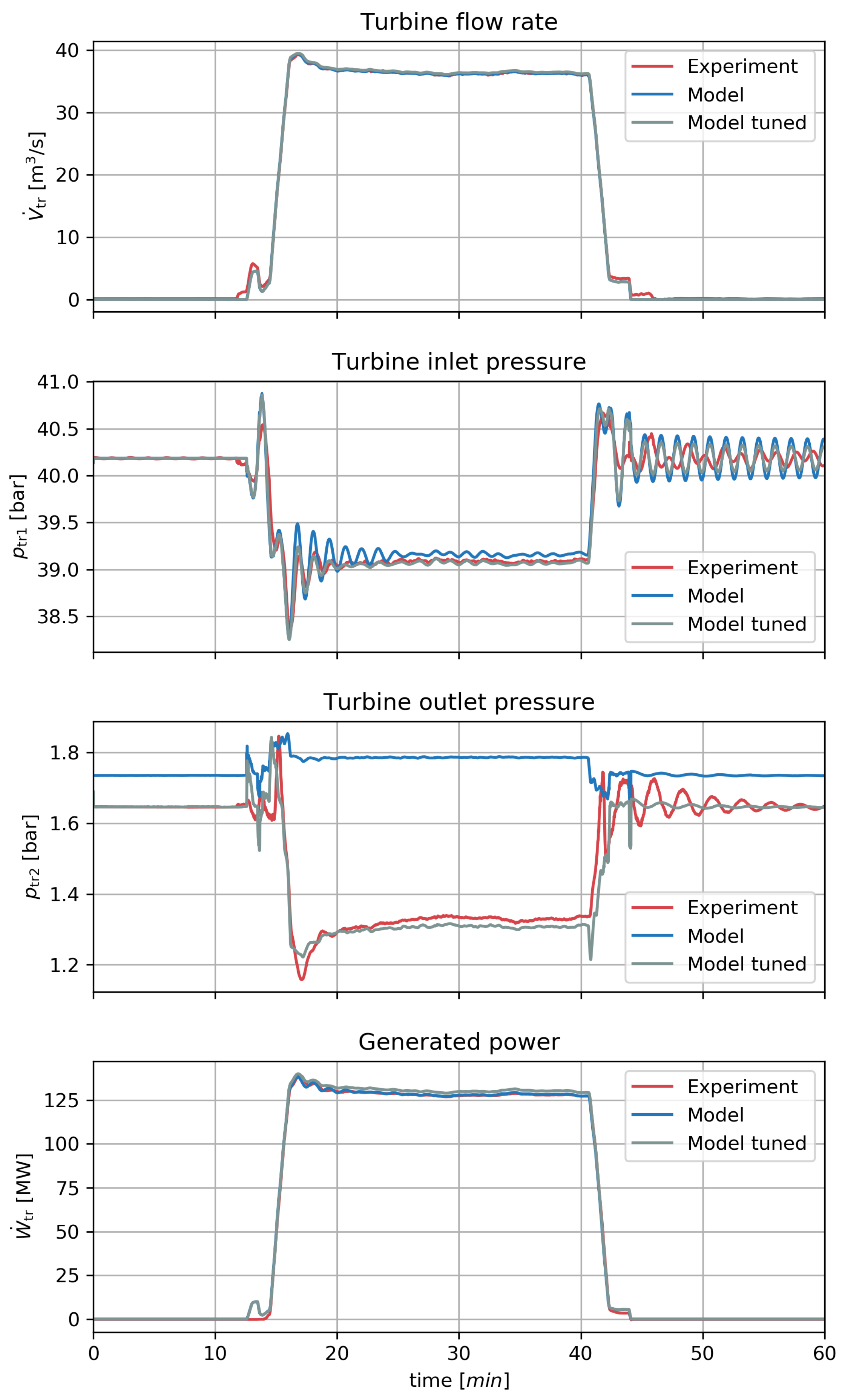
It is seen from Figure 9 that the tuned model provides good results that fit the measured data reasonably well. Some deviation in pressure oscillations is still visible, but the results look promising and are greatly improved in comparison to the results from the original model (Figure 6). This improvement is also confirmed by the root mean squared error between the model and experiment curves. The RMSE has been reduced for the turbine inlet pressure from 0.142 to 0.101 bar, and for the turbine outlet pressure from 0.315 to 0.04 bar. For the the turbine flow rate and the generated power, the RMSE has not been changed significantly.
4.4. Detailed Hydropower Models
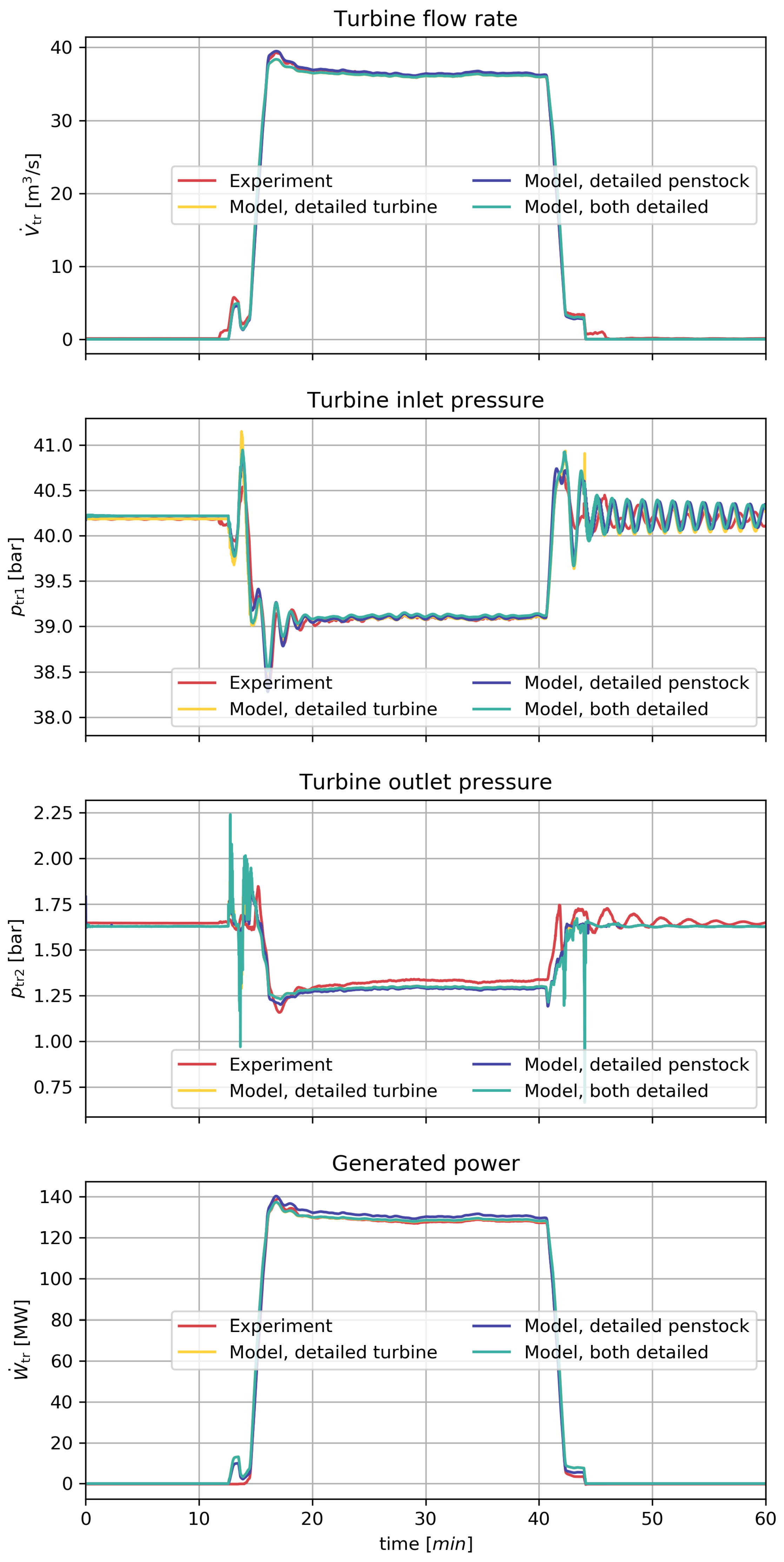
Thus, far, the model tuning has been based on extending the simple model (model #1 in Section 3.2) with a draft tube. It is of interest to compare the experimental measurements with the simulation results from the other hydropower models (models #2–#4 in Section 3.2), with friction coefficient expressions from Section 4.2.2 and tuned parameters from Section 4.3.3, where appropriate. For the cases involving a detailed penstock model, each of the PenstockKP elements (for two penstock units) is set with five discretization segments. The simulations are performed for the same operational conditions and the same scenario as during the experiment.
Comparison of the simulation results from these more detailed model cases with the measured data is shown in Figure 10. Similarly to the previous simple model simulations, Figure 10 provides four plots: the turbine flow rate, the turbine inlet and outlet pressures, and the generated power.
Figure 10 shows that the results from the more detailed hydropower models look similar and fit the experimental data relatively well. Some extra oscillations for the outlet pressure exist for the cases with the mechanistic Francis turbine model. These oscillations are caused by the turbine model uncertainties when the zero load regime is reached. Moreover, the presented results from the more detailed hydropower models do not show a significant difference from the results with the simple model case (Figure 9). Because of this, we do not further tune the parameters in the more detailed models.
5. Discussion
In this paper, the use of the open-source Modelica library OpenHPL for hydropower system modelling has been presented. OpenHPL provides models at different levels of complexity of hydropower system units which can be used to create a model of a hydropower system, depending on the user’s needs. Models of various complexity levels have been presented in this study for the case of the Trollheim hydropower plant. The experimental data from the hydropower plant have been presented and discussed.
The experimental data were first used for library element tuning, in tuning the friction loss coefficients of the Francis turbine model (the Francis element). Based on the resulting values of friction loss coefficients in this paper and in previous work, it was observed that there appears to be simple relationships between friction coefficients and the turbine nominal head. Expressions relating the nominal head and the friction coefficients have been proposed, which allows for an improvement of the Francis turbine design algorithm presented in [23].With the friction coefficient expressions in Section 4.2, the turbine model can be completely specified by knowledge of nominal turbine head and nominal flow rate through the turbine. Further work to validate these expressions should be carried out.
Next, a simple model (table look-up turbine model, incompressible water, inelastic pipes) was extended with a simplified draft tube for the turbine, and it was demonstrated that, by tuning the friction roughness heights of the pipes and the geometry of the draft tube, good model fit to experimental data was achieved. Model fit was achieved by first manually tuning model parameters in order to gain an understanding of the importance of parameters, and next by using the manually fitted parameters as initial guesses in multiparametric least squares fitting. Tuning of the roughness height (and thereby the friction energy loss) affects the transient amplitude/oscillations while the geometry of the draft tube has strong implications for the turbine outlet pressure. Correct description of the turbine outlet pressure is essential for avoiding cavitation.
Finally, more detailed hydropower models have been equipped with the model parameters from the simple model and simulation results have been compared with the experimental data. The results indicate that these more complex models also exhibit good model fitting. Some minor deviation between the models and measured results exists, but this deviation is believed to be relatively insignificant. The fact that the model parameters from the simple model generalizes well to the more complex models indicates that the model variables/parameters can be given a physical interpretation.
Overall, the developed models using OpenHPL look promising and might find the following uses for hydropower systems:
- Modelling and simulation [21],
- State estimation/smart sensor that enables estimation of unmeasured states/parameters based on combining models and available measurements [37],
- Linearization for control design [28],
- Advanced control design and testing, e.g., model predictive control (MPC),
- Integration of waterway model with electric grid model by combination with power system libraries, e.g., Open-Instance Power System Library (OpenIPSL [38]),
- Large scale control analysis, for example, based on a graph theory.
6. Conclusions
At the outset, some research questions were posed. Based on the results in this paper, we have confirmed that, by proper tuning, OpenHPL is suitable for describing real hydropower plants with little prior plant knowledge. Except for the turbine outlet pressure, the original model gave realistic predictions of the hydropower plant performance. This implies that future work should be put into developing improved models for the draft tube, with good default geometry parameters based on nominal turbine height and flow rate. The developed expressions for Francis turbine friction coefficients should be tested further. In addition, OpenHPL should be extended with models for other turbine types.
Because OpenHPL is based on the multiphysics language Modelica, available libraries for modelling the electric grid make it possible to model and study regional hydropower systems, but also to integrate the study with other, renewable energy sources when Modelica libraries for these other energy sources become available.
Integration of simulation tools such as OpenModelica with scripting languages such as Python and Julia allows for model based analysis and synthesis in a simple and straightforward way. Furthermore, by basing the tool chain on open source tools, this makes it simple to use these tools in education, and allows for contributions and extensions from the community of users.
Author Contributions
Both authors have significant contribution in the paper and more detailed individual contributions are specified here: conceptualization, L.V. and B.L.; methodology, L.V.; software, L.V.; validation, L.V; formal analysis, L.V. and B.L.; investigation, L.V. and B.L.; writing—original draft preparation, L.V.; writing—review and editing, B.L.; visualization, L.V.; supervision, B.L.
Funding
This research received no external funding.
Acknowledgments
Erik Jacques Wiborg from Statkraft Energi AS, Oslo, Norway, provided the experimental and other related data from the Trollheim power plant for the case study. Bjarne Børresen from Multiconsult AS, Oslo, Norway helped put us in touch with Erik Wiborg. This is gratefully acknowledged.
Conflicts of Interest
The authors declare no conflict of interest.
References
- Munoz-Hernandez, G.; Mansoor, S.; Jones, D. Modelling and Controlling Hydropower Plants; Advances in Industrial Control; Springer: London, UK, 2013. [Google Scholar]
- Nielsen, T.K. Transient Characteristics of High-Head Francis Turbines. Ph.D. Thesis, Norwegian University of Science and Technology, Trondheim, Norway, 1990. [Google Scholar]
- Yang, W.; Yang, J.; Guo, W.; Zeng, W.; Wang, C.; Saarinen, L.; Norrlund, P. A Mathematical Model and Its Application for Hydro Power Units under Different Operating Conditions. Energies 2015, 8, 10260–10275. [Google Scholar] [CrossRef]
- Fang, H.; Chen, L.; Dlakavu, N.; Shen, Z. Basic Modeling and Simulation Tool for Analysis of Hydraulic Transients in Hydroelectric Power Plants. IEEE Trans. Energy Convers. 2008, 23, 834–841. [Google Scholar] [CrossRef]
- Guo, W.; Yang, J.; Yang, W.; Chen, J.; Teng, Y. Regulation quality for frequency response of turbine regulating system of isolated hydroelectric power plant with surge tank. Int. J. Electr. Power Energy Syst. 2015, 73, 528–538. [Google Scholar] [CrossRef] [Green Version]
- Yang, W.; Norrlund, P.; Bladh, J.; Yang, J.; Lundin, U. Hydraulic damping mechanism of low frequency oscillations in power systems: Quantitative analysis using a nonlinear model of hydropower plants. Appl. Energy 2018, 212, 1138–1152. [Google Scholar] [CrossRef]
- Quiroga, O.; Riera, J.; Batlle, C. Identification of partially known models of the Susqueda hidroelectric power plant. Lat. Am. Appl. Res. 2003, 33, 387–392. [Google Scholar]
- Margonis, P. Modeling and Optimization of a Hydroelectric Power Plant for a National Grid Power System Supply. Case Study: Stratos Hydroelectric Dam. Ph.D. Thesis, Technical University of Crete, Chania, Greece, 2017. [Google Scholar]
- LVTrans. Open Source Transient Simulations Software for Hydraulic Piping Systems. Available online: http://svingentech.no/index.html (accessed on 14 June 2019).
- National Instruments. LabVIEW 2019. Available online: http://www.ni.com/en-no/shop/labview/labview-details.html (accessed on 14 June 2019).
- Sandvåg, S.U. Surge Tank Atlas for Hydropower Plants. Master’s Thesis, Department of Hydraulic and Environmental Engineering, Norwegian University of Science and Technology, Trondheim, Norway, 2016. [Google Scholar]
- Yang, W. Hydropower Plants and Power Systems: Dynamic Processes and Control for Stable and Efficient Operation. Ph.D. Thesis, ElectricityElectricity, Uppsala University, Uppsala, Sweden, 2017. [Google Scholar]
- École Polytechnique Fédérale de Lausanne (EPFL). Simulation Software for Power Networks SIMSEN. Available online: https://simsen.epfl.ch (accessed on 14 June 2019).
- Nicolet, C. Hydroacoustic Modelling and Numerical Simulation of Unsteady Operation of Hydroelectric Systems. Ph.D. Thesis, École Polytechnique Fédérale de Lausanne, Lausanne, Switzerland, 2007. [Google Scholar]
- Modelon. Hydro Power Library. Available online: https://www.modelon.com/library/hydro-power-library (accessed on 14 June 2019).
- Modelon. System Simulation without Boundaries. Available online: https://www.modelon.com (accessed on 14 June 2019).
- Dassault Systems. DYMOLA Systems Engineering. Available online: https://www.3ds.com/products-services/catia/products/dymola (accessed on 14 June 2019).
- Winkler, D.; Thoresen, H.M.; Andreassen, I.; Perera, M.A.S.; Sharefi, B.R. Modelling and Optimisation of Deviation in Hydro Power Production. In Proceedings of the 8th International Modelica Conference, Linköping Electronic Conference, Dresden, Germany, 20–22 March 2011; Volume 1. [Google Scholar]
- Tuszynski, K.; Tuszyński, J.; Slättorp, K. HydroPlant–a Modelica Library for Dynamic Simulation of Hydro Power Plants. In Proceedings of the 5th International Modelica Conference, Vienna, Austria, 4–5 September 2006; Volume 1. [Google Scholar]
- OpenModelica. Available online: https://openmodelica.org (accessed on 14 June 2019).
- Vytvytskyi, L.; Lie, B. Comparison of elastic vs. inelastic penstock model using OpenModelica. In Proceedings of the 58th Conference on Simulation and Modelling, Reykjavik, Iceland, 25–27 September 2017; Volume 138, pp. 20–28. [Google Scholar] [CrossRef]
- Splavska, V.; Vytvytskyi, L.; Lie, B. Hydropower Systems: Comparison of Mechanistic and Table Look-up Turbine Models. In Proceedings of the 58th Conference on Simulation and Modelling, Reykjavik, Iceland, 25–27 September 2017; Volume 138, pp. 368–373. [Google Scholar] [CrossRef]
- Vytvytskyi, L.; Lie, B. Mechanistic model for Francis turbines in OpenModelica. IFAC-PapersOnLine 2018, 51, 103–108. [Google Scholar] [CrossRef]
- Modelica. The Modelica Association. Available online: https://www.modelica.org (accessed on 14 June 2019).
- OpenModelica. OpenModelica Python Interface and PySimulator. Available online: https://www.openmodelica.org/doc/OpenModelicaUsersGuide/latest/ompython.html (accessed on 14 June 2019).
- Python. Available online: https://www.python.org (accessed on 14 June 2019).
- Lie, B.; Bajracharya, S.; Mengist, A.; Buffoni, L.; Kumar, A.; Sjölund, M.; Asghar, A.; Pop, A.; Fritzson, P. API for Accessing OpenModelica Models From Python. In Proceedings of the EuroSim 2016, Oulu, Finland, 12–16 September 2016. [Google Scholar]
- Vytvytskyi, L.; Lie, B. Linearization for Analysis of a Hydropower Model using Python API for OpenModelica. In Proceedings of the 59th Conference on Simulation and Modelling, Oslo, Norway, 26–27 September 2018; Volume 153, pp. 216–221. [Google Scholar] [CrossRef]
- Statkraft. Trollheim Hydropower Plant. Available online: https://www.statkraft.com/energy-sources/Power-plants/Norway/Trollheim (accessed on 14 June 2019).
- Wiborg, E.J. Continuous Efficiency Measurements on Hydro Power Plants. Ph.D. Thesis, Norwegian University of Science and Technology, Trondheim, Norway, 2016. [Google Scholar]
- GitHub. Trollheim Experiment. Available online: https://github.com/liubomyrv/TrollheimExperiment.git (accessed on 14 June 2019).
- Tiller, M.M. Modelica by Example. Available online: http://book.xogeny.com (accessed on 14 June 2019).
- OpenModelica. User Documentation. Available online: https://openmodelica.org/useresresources/userdocumentation (accessed on 14 June 2019).
- The National Programme on Technology Enhanced Learning (NPTEL). Francis Turbine. Available online: https://nptel.ac.in/courses/Webcourse-contents/IIT-KANPUR/machine/chapter_7/7_7.html (accessed on 14 June 2019).
- SciPy. Numpy and Scipy Documentation. Available online: https://docs.scipy.org/doc (accessed on 14 June 2019).
- EnggCyclopedia. Absolute Pipe Roughness. Available online: https://www.enggcyclopedia.com/2011/09/absolute-roughness (accessed on 14 June 2019).
- Vytvytskyi, L.; Lie, B. Combining Measurements with Models for Superior Information in Hydropower Plants. Flow Meas. Instrum. 2019, accepted. [Google Scholar]
- GitHub. OpenIPSL: Open-Instance Power System Library. Available online: https://github.com/OpenIPSL/OpenIPSL (accessed on 14 June 2019).
Figure 1.
Overview of the structure of the high head hydropower plant.

Figure 2.
Measurements of the experimental conditions.

Figure 3.
Flow sheet of the model of the hydropower system in OpenModelica. Modelled using OpenHPL.

Figure 4.
Comparison of the model simulation and experimental power vs. turbine flow rate characteristics.
Figure 4.
Comparison of the model simulation and experimental power vs. turbine flow rate characteristics.

Figure 5.
Linear relationship between natural logarithm of the turbine loss coefficients, and and the nominal head.
Figure 5.
Linear relationship between natural logarithm of the turbine loss coefficients, and and the nominal head.

Figure 6.
Comparison of the simple hydropower model simulation results and the experimental data.

Figure 7.
Comparison of the turbine inlet pressure from the simple model simulations with individual settings and experimental measurements.
Figure 7.
Comparison of the turbine inlet pressure from the simple model simulations with individual settings and experimental measurements.

Figure 8.
Comparison of the turbine outlet pressure from the simple model simulations with different draft tube (DT) settings and experimental measurements.
Figure 8.
Comparison of the turbine outlet pressure from the simple model simulations with different draft tube (DT) settings and experimental measurements.

Figure 9.
Comparison of the results from the tuned simple hydropower model (with tuned draft tube and roughness) and the experimental data.
Figure 9.
Comparison of the results from the tuned simple hydropower model (with tuned draft tube and roughness) and the experimental data.

Figure 10.
Comparison of the results from the detailed hydropower models and the experimental data.


Table 1.
The waterway geometry; Trollheim plant.
| Waterway Unit | Height Difference, () | Length, () | Diameter, () |
|---|---|---|---|
| Reservoir | 46.5 | – | – |
| Intake race #1 | 9 | 81.5 | 6.3 |
| Intake race #2 | −2 | 395 | 6.3 |
| Intake race #3 | 9 | 4020 | 6.3 |
| Penstock #1 | 233 | 363 | 4.7 |
| Penstock #2 | 105 | 145 | 3.3 |
| Surge tank | 75.5 | 87 | 3.4 |
| Discharge race #1 | 3.5 | 601 | 6.3 |
| Discharge race #2 | −8.6 | 21 | 6.3 |
Table 2.
The turbine nominal operational values; Trollheim plant.
| Turbine Type | Nominal Head () | Nominal Flow Rate () | Nominal Power () | Nominal Rotational Speed () |
|---|---|---|---|---|
| Francis | 371 | 37 | 130 | 37 |
Table 3.
Measured quantities.
| Quantity Name | Symbol | Information |
|---|---|---|
| Turbine guide vane control signal | Model input | |
| Turbine rotational speed | ||
| Water level in the tail water | ||
| Turbine inlet pressure | Model output | |
| Turbine outlet pressure | ||
| Turbine volumetric flow rate | ||
| Generated power |
Table 4.
The waterway parameters tuned with the least squares error method.
| Waterway Unit | Roughness Height, , () |
|---|---|
| Intake race #1 | 0.01 |
| Intake race #2 | 0.014 |
| Intake race #3 | 0.59 |
| Penstock #1 | 0.16 |
| Penstock #2 | |
| Surge tank | |
| Disch. race #1 | 0.027 |
| Disch. race #2 | 0.01 |
Table 5.
The draft tube pipe parameters tuned with the least squares error method.
| Waterway Unit | Roughness Height, , () | Expand Diameter, () | Length, () |
|---|---|---|---|
| Draft tube | 2.18 → 3.01 | 12 |
© 2019 by the authors. Licensee MDPI, Basel, Switzerland. This article is an open access article distributed under the terms and conditions of the Creative Commons Attribution (CC BY) license (http://creativecommons.org/licenses/by/4.0/).
Share and Cite
MDPI and ACS Style
Vytvytskyi, L.; Lie, B. OpenHPL for Modelling the Trollheim Hydropower Plant. Energies 2019, 12, 2303. https://doi.org/10.3390/en12122303
AMA Style
Vytvytskyi L, Lie B. OpenHPL for Modelling the Trollheim Hydropower Plant. Energies. 2019; 12(12):2303. https://doi.org/10.3390/en12122303
Chicago/Turabian StyleVytvytskyi, Liubomyr, and Bernt Lie. 2019. "OpenHPL for Modelling the Trollheim Hydropower Plant" Energies 12, no. 12: 2303. https://doi.org/10.3390/en12122303
Note that from the first issue of 2016, this journal uses article numbers instead of page numbers. See further details here.