Hourly CO2 Emission Factors and Marginal Costs of Energy Carriers in Future Multi-Energy Systems


1
Forschungsstelle für Energiewirtschaft (FfE) e.V., 80995 München, Germany
2
Department of Electrical and Computer Engineering, Technical University of Munich (TUM), 80333 München, Germany
*
Author to whom correspondence should be addressed.
Energies 2019, 12(12), 2260; https://doi.org/10.3390/en12122260
Submission received: 9 May 2019
/
Revised: 7 June 2019
/
Accepted: 10 June 2019
/
Published: 13 June 2019
(This article belongs to the Special Issue Model Coupling and Energy Systems)
Abstract
:Hourly emission factors and marginal costs of energy carriers are determined to enable a simplified assessment of decarbonization measures in energy systems. Since the sectors and energy carriers are increasingly coupled in the context of the energy transition, the complexity of balancing emissions increases. Methods of calculating emission factors and marginal energy carrier costs in a multi-energy carrier model were presented and applied. The model used and the input data from a trend scenario for Germany up to the year 2050 were described for this purpose. A linear optimization model representing electricity, district heating, hydrogen, and methane was used. All relevant constraints and modeling assumptions were documented. In this context, an emissions accounting method has been proposed, which allows for determining time-resolved emission factors for different energy carriers in multi-energy systems (MES) while considering the linkages between energy carriers. The results showed that the emissions accounting method had a strong influence on the level and the hourly profile of the emission factors. The comparison of marginal costs and emission factors provided insights into decarbonization potentials. This holds true in particular for the electrification of district heating since a strong correlation between low marginal costs and times with renewable excess was observed. The market values of renewables were determined as an illustrative application of the resulting time series of costs. The time series of marginal costs as well as the time series of emission factors are made freely available for further use.
1. Introduction
Future energy systems will be characterized by increased volatility in electricity generation due to variable renewable energy sources (vRES) as well as stronger linkages between energy carriers. These new interdependencies derive from the coupling of previously separate energy carriers in multi-energy systems (MES), as defined in [1] by means of technologies such as power-to-heat (PtH) and power-to-gas (PtG). Therefore, when assessing future energy technologies with regard to CO2 emissions, not only the time of energy consumption and generation need to be considered, but also the linkages between energy carriers need to be accounted for.
In recent studies dealing with the decarbonization of the German energy system (e.g., [2,3,4]), the focus lies on describing changes in absolute emissions. There are some studies available, (e.g., [5,6]) which demonstrate the resulting specific emission factor for the annual electricity mix. However, there are very few analyses on the future German energy system which report the specific emission factor of electricity with a high time resolution, much less for other energy carriers.
An overview of different approaches to quantify emission factors of electricity is provided by [7]. The existing methods differ with regard to the input data and the models used (empirical data and statistical relationship models vs. power system optimization models), the time horizon (historical vs. future), the temporal resolution (from less than one hour to one year), the consideration of imports and exports as well as the regional differentiation. Whereas in several analyses, e.g., [8,9], methods are presented to determine hourly average and marginal emission factors of electricity based on power system optimization models, the work on integrating these methods into the modeling of MES is limited. Considering the increasing integration of various energy carriers in future MES, these methods need to be expanded from electricity and district heating to other energy carriers such as methane and hydrogen. In this context, the allocation of emissions to multiple strongly interconnected energy carriers is the main challenge to be solved. To understand the interdependencies and operational incentives of the modeled future energy system, it is helpful to supplement the time-resolved emission factors with an examination of hourly marginal energy carrier costs.
This study provides a methodology and a data set for specific emission factors and marginal costs of different energy carriers for a future German MES scenario with high time resolution. This data is required when determining the CO2 emissions of future energy technologies while also considering the dependency of emissions on the load profile and on linked energy carriers. Since load management strategies will play an increasing role in balancing supply and demand in future energy systems, the time series of emission factors provided can also serve as an input for the development of load management strategies aimed at CO2 emission reduction. An estimation of the economic feasibility of these measures can be carried out by combining the resulting emission factors with the hourly marginal generation costs.
2. Methods
The methodological approach consists of four building blocks. First, the modeling approach of the MES is described in Section 2.1. This model is then applied to simulate the future energy system for the scenario described in Section 2.2. In this section, the scope of the analysis is defined and the associated input data is outlined. Furthermore, the energy balances resulting from the simulation of the described scenario with the MES model are evaluated and discussed for the modeled energy carriers. In a third step, the methods for balancing emissions by energy carrier and calculating hourly emission factors from the generated scenario results are presented in Section 2.3. Finally, the procedure to determine hourly marginal costs of energy carriers, which also builds on the results of the simulated future MES scenario, is described in Section 2.4.
2.1. Multi-Energy System Model
The MES model used and modified for this analysis is called “ISAaR, Integriertes Simulationsmodell zur Anlageneinsatz-und Ausbauplanung mit Regionalisierung”, with the German abbreviation standing for the term “Integrated simulation model for plant operation and expansion planning with regionalization”. ISAaR is a model based on the mathematical method of linear optimization with the optimization goal of minimizing overall system cost . A detailed description of the model is given below. In addition, individual input datasets, model components and application examples are presented in publications like [10,11,12,13,14,15].
The equations of ISAaR are based on linear optimization, a method described in detail in works such as [16,17]. The general equations are noted in the following in order to define notations and terms. The model-specific equations can be found in the subsequent sections.
A linear optimization problem is formed by:
The vector of variables is to be optimized. The vector contains the specific costs of the variable vector . All system dependencies are described within the constraint matrix , the left and right boundary of the constraints and , and the lower and upper bounds of the variables and .
Using this approach, a MES is described by the ISAaR model. The selection of relevant energy carriers is made with a focus on future decarbonization strategies in the German energy system. Key studies used as benchmarks are [2,4,5]. As a result, the energy carriers of electricity, district heating, hydrogen, methane, and biomass are selected. For the consideration of more ambitious decarbonization paths, carbon-based liquid energy carriers are also implemented in a simplified manner. Figure 1 shows the energy carriers considered, the conversion technologies, and the boundaries of the system.
All optimization runs are performed in hourly resolution but not all energy carriers are resolved hourly (see Figure 1). Energy carriers with sufficient storage capability (i.e., hydrogen or methane) are taken into account in annual or daily totals. The weather year used in order to generate load or renewable profiles is 2012. With respect to the German power system, 2012 was an average weather year regarding to temperatures and renewable generation potential [18]. Whereas all energy carriers shown are modeled in detail for the German region, the neighboring countries are considered in a simplified manner. Electricity generation is modeled taking aggregated conventional power plant blocks, hydro storages, and renewables into account. As shown in Figure 1, four different classes of energy system elements are distinguished: generation, conversion, storage and import/export elements. In principle, the elements of “generation” and “import or export” are very similar as energy carrier flows across system boundaries are taken into account in both cases. In contrast, the elements “storage” and “conversion” do not cross the system boundaries. Storage elements provide a temporal offset between charging and discharging without converting the energy carrier. In the case of conversion, a transformation of energy carriers takes place in which emissions can occur during combustion or can be withdrawn from the system. An example for a withdrawal is the absorption of CO2 from the air to synthesize methane (“Power-to-methane”).
In the following, the mathematical foundations of the model are described in more detail. With regard to the nomenclature for the following explanations, it should be noted that an “element” constitutes a designation for a group of technically similarly operating units whose functionality is modeled by the same set of mathematical equations. The individual plant is referred to as a “unit”.
2.1.1. System Constraints
The system constraints link several generation technologies , conversion technologies and storage systems , thus ensuring load fulfilment of a specific energy carrier per final energy consumption (FEC) sector for every time step and in every region under consideration. Striked subscripts represent a link to another energy carrier or region . The input or output power of generating, storing or converting devices is modeled in addition to imported or exported energy. The breakdown of this hourly power balance is shown in Equation (2).
The load is assumed to be inflexible. All price-sensitive load components are modeled as flexibility options (e.g., as storage) or in the context of previous profile generation within the FEC sector models (e.g., photovoltaic (PV) home storage for self-supply).
2.1.2. Conversion and Generation Technologies
The equations representing conversion technologies (e.g., electrolyzers) and power plant operation are described as follows. The first step is the reference case of a typical conversion or generation process with one input and one output energy carrier including the conversion or generation efficiency .
For all instances, their maximum generation capacity is limited by the individual rated power capacity and the average operational availability for this technology type.
If no availability is given, is set to 1, and the upper bound of equals These bounds of the operational variables apply equally to the power drawn and the storage level .
Due to the high relevance with regard to the resulting power plant dispatch and, therefore the determination of marginal generation costs and emission factors, a high level of detail is applied for modeling conventional electricity generators. Therefore, the above equations are modified for conventional power plants. The chosen approach is mainly based on the modeling equations shown in [19]. This approach is also used for the linearization of fuel consumption in power plants, which, take partial load behavior and start-up costs into account. In view of the complexity and the large scope of this mathematical description, this section can be found in Appendix A.
An exception requiring an element-specific modeling is the addition of hydrogen to the natural gas network . For this purpose the imported methane , the methane in- and output of natural gas storages as well as electrolysis and methanization units are balanced.
Although the load condition of the energy carrier methane is to be fulfilled daily, the output variables are determined in hourly resolution. Based on the findings in [20] the maximum volumetric addition factor is set to 10%.
2.1.3. Storage Processes
A linear optimization approach for modeling e.g., a hydro pumped storage power plant, is described in [21]. A characteristic is the temporal coupling between the optimized variables of the SoC (State of Charge). The self-discharge of a storage system is integrated by the loss coefficient . Based on these definitions, the following condition can be derived for hydro, thermal, methane and battery storage systems:
A detailed description of the modeling of seasonal hydro and pumped storage systems with natural inflow is provided in [14].
2.1.4. Software
All input data is stored in a PostgreSQL database. The problem formulation and result processing is carried out in a standardized procedure in MATLAB®. The optimization problem is solved by IBM® CPLEX using the barrier algorithm.
2.2. Energy System Scenario
The research focus of the Dynamis project is the assessment of various CO2 abatement measures with regard to cost efficiency using energy system modeling. In order to evaluate these measures for decarbonization, it is first necessary to create a reference path as a starting point in order to be able to evaluate deviating and strongly decarbonizing paths. In the following, this reference scenario, which is the object of the examinations documented here, is referred to as the “Dynamis Start Scenario”. The time horizon of the analysis extends in five-year steps from the year 2020 to the year 2050. The regional scope of the analysis is the German grid area. The influence of the 34 surrounding European ENTSO-E (European Network of Transmission System Operators for Electricity) regions, which mostly correspond to countries, are also considered. The list of countries can be found in Appendix B. The input data and assumptions regarding the development of emission certificate prices and fuel prices as well as emission factors related to the combustion processes of the energy carriers considered are included in Appendix C. In order to create a current reference scenario, it is necessary to merge different sources. The studies used for this purpose are listed Table 1 and classified according to their scope and suitability.
The scenario considered here is made up of individual components from the sources outlined above. The components are selected on the basis of Table 1 with the aim of using the highest level of detail of available input data for each area. Overall, it may be noted that an essential part of the scenario data for generation in Germany originates from the NEP (“Netzentwicklungsplan 2019”, German Network Development Plan 2019). These values are updated by the findings of the German “Coal Commission” [24]. For the NEP and the TYNDP (Ten-Year Network Development Plan 2018 of ENTSO-E), a linear extrapolation up to the year 2050 is conducted to complete the available datasets on the generation side. The discontinuity in consistency with the load data coming from the ERP (energy reference projection) is accepted in favor of actuality. Given the background of an adjusted political environment and the associated strong change in the growth of vRES it appears appropriate to update generation capacities. German demand data, on the other hand, is based on ERP since it is the most recent study providing a detailed breakdown of the FEC sectors. This granular breakdown of consumption sectors is needed because a bottom-up modeling of FEC sectors is being carried out in the context of the Dynamis project. Using this approach, sectoral load profiles can be generated and then specific decarbonization measures, e.g., the transition to electric heating systems in private households, can be assessed. In some areas, there have been developments on the consumption side, which require small deviations from the 2014 ERP scenario data. Large deviations due to efficiency or electrification measures are not considered in this work. Overall, the scenario is of a conservative nature.
In the following sections, for each modelled energy carrier, the processing of input datasets and the resulting scenario data for energy carrier generation and consumption are elaborated on. In addition, the energy carrier balances resulting from the simulation of the scenario are described.
2.2.1. Electricity
Based on the scenario values for installed capacity in the respective years, a decommissioning and expansion planning process is carried out for individual fossil-fired power plant units. This is done until the scenario capacity specifications are met. In neighboring European countries, the PLATTS power plant database [25] is used for conventional power plant unit data. Since the modeling in the surrounding countries is only regarded as a boundary condition for the detailed German consideration, power plant units in these countries are aggregated based on the efficiencies, turbine type and fuel type of the power plants. These power plant data are clustered as follows: First, the individual turbines of a combined-cycle unit are merged. Second, efficiencies are assigned to all units. For this purpose, manually searched turbine model-specific efficiencies are used. Standard efficiencies according to TYNDP are used for the remaining power plant units that are not covered. The TYNDP data are prepared in order to assign the various ranges of values to the age classes of the power plants. Decommissioning is carried out according to the age of the power plants described in [25]. In general, only the same power plant technologies (combined cycle gas turbine, gas turbine, hard-coal steam turbine, lignite steam turbine, nuclear) are grouped within one country. The maximum allowed efficiency deviation from the mean value of a cluster is set to 0.5% and the maximum aggregated unit size is 2 GW. An illustrative analysis of clustering for the year 2030 shows that the number of units in the European surrounding countries can be reduced from ~1200 to ~800 units. The resulting change in the average electricity price in Germany is below 0.1% and the deviation in dispatch of conventional power plants is below 0.2%.
As described above, the development of the generation capacities is extrapolated from the TYNDP. This assumption may lead to capacity shortages in system adequacy in some countries. Therefore, an exception is made for those countries for which these shortages have been identified in an annual calculation. In this case, the 2040 values are kept at a constant level and no further reduction in capacity due to the extrapolation is made. In this particular case, the countries concerned are Bulgaria, Macedonia, Slovakia, Romania, Hungary, Czech Republic, Greece, Northern Ireland, and Hungary.
Another adjustment is the update due to the German coal phase-out. The NEP coal capacities are replaced by the Commission’s values for the years 2022 and 2030, as well as 2038. Intermediate data points are interpolated. Decommissioning of individual units takes place as follows.
For Germany power plant units are not being clustered. The unit data is taken from the “BNetzA” (Federal Network Agency for Electricity, Gas, Telecommunications, Post and Railway) power plant list [26], which includes the planned construction, retrofitting, and decommissioning of power plants [27]. Another data source is the UBA power plant database [28] for combined heat and power (CHP) plants in particular. In addition, the individual units are provided with manually searched data on nominal output, thermal district heating output, efficiency and CHP technology. Decommissioning is based on the age of the power plant and the district heating output. If, according to scenario data, there is a need to decommission a coal-fired CHP plant in Germany, this unit is replaced by a gas-fired unit. The district heating output capacity is kept constant. In the case of a backpressure steam turbine CHP plant in a district heating network, this plant is replaced by a gas combined-cycle backpressure turbine plant. In principle, the reported planned shutdowns are decommissioned first, followed by the oldest power plants.
Industrial power plants are modeled according to their operating incentive. In addition to the feed-in into the public grid, this includes either the supply of process heat or district heating, the industrial auto-production or the combustion of industrial waste products (e.g., blast furnace gas). A detailed description of data and modeling approach can be found in [15,29]. Small gas-fired cogeneration plants under 10 MW are taken into account for the year 2020 to the extent of 4.3 GW. It is assumed that the installed capacity will double by 2050.
Due to the adjustments of the NEP scenario B capacity data by the coal phase-out, the system faces a capacity shortage. For this reason, an integrated expansion planning of gas-fired units is carried out. According to [30,31,32], the assumed values for gas turbine power plants are 35 years of service life, an electrical efficiency of 40%, an investment of €408,750 per MW, as well as fixed operating costs of €54,029 per MW and year. The social discount rate for developed countries of 3.5% from [33] is assumed in order to determine the annuities of investments.
In the context of the analysis presented here, there is no further investigation of system adequacy. The energy system described works under the conditions of the weather year 2012. Therefore, it should be noted that times when neither solar nor wind generation are available for a longer period than in the weather year 2012 are not considered. This also applies to the hypothetical simultaneous failure of several power plant capacities. An increased installed capacity of gas turbines or engines would be necessary for ensuring system adequacy in such cases. However, since these units would only be used as a backup, thus producing very few full load hours, their repercussions on emissions and emission factors are negligible. To address this undetermined demand for backup capacities, this demand for backup capacities is included in Figure 2 as an unspecified element. All capacities shown are gross capacities. The availability of the plants is assumed according to the values of the “TYNDP unit data” [22].
A two-stage approach is used for the most important renewables, namely hydro, wind and solar. First, the scenario data according to NEP and TYNDP is regionalized. Based on the locations of existing plants, geo-analysis, weather data and local expansion goals, vRES expansion differentiated by location and plant type is carried out. Then the plant characteristic curves are intersected with the weather data of the respective location to generate a generation profile. Whereas the data used for wind and PV systems are described in the following, hydro systems are described in [15]. The generation profiles for photovoltaic systems are based on a model that processes weather data and takes into account technical parameters such as low-light panel performance and inverter efficiency. The model uses radiation data from the Copernicus Atmosphere Monitoring Service (CAMS) [34], containing information on the direct and diffuse components of global radiation. The temporal resolution is from 1 to 15 min. Furthermore the weather parameters of ambient temperature and albedo are taken from the COSMO-EU model [35]. In addition, the COSMO-EU radiation data from the Scandinavian countries are used since, with the exception of Denmark, they are not part of the CAMS dataset. Since the COSMO-EU model does not contain information on the direct and diffuse components of global radiation, this information is derived from the global radiation and the clear sky index. The temporal resolution is one hour. The generation profiles can be calculated for different inclinations and orientations of solar panels.
The generation profiles for wind turbines are based on data from the COSMO-EU weather model DWD [35]. This model includes the wind speeds on a 7.5 km grid at different heights. Regional wind profiles are calculated based on the power curves of different manufacturers and turbine types. A typical plant type must be determined for each NUTS-3 region. Five different types are considered, which differ in their power curves and thus represent the various turbine types for weak to strong winds. The full load hours are calculated for each of the five turbines. Starting from the turbine type for strong winds, it is checked whether a minimum of full load hours can be achieved in this NUTS-3 region. If the strong wind turbine does not meet this minimum requirement, then the turbine types for weaker winds are tested step by step. For the first two turbine types, the minimum requirement of full load hours is 2500 h/a, for the other 1600 h/a.
Due to the growing exploitation of suitable locations, for wind onshore and PV, less suitable locations are being explored over time because the overall penetration is increasing. In the case of wind onshore, this development is overcompensated for by higher hub heights and larger rotor blades. The full load hours of wind onshore will increase on average from 1890 h/a in 2020 to 2280 h/a in 2050. In the same period, the values of PV will fall slightly from 980 h/a to 970 h/a. For offshore wind, this effect will not occur, and full load hours will remain constant at 4570 h/a.
In contrast to conventional generation technologies, renewables (solar, wind and run-of-river) are not being dispatched within the optimization. vRES generation profiles are calculated exogenously and fed into the system as an generation, which is assumed to be generated at a marginal cost of 0 €/MWh. This allows curtailment if doing so is necessary or cost efficient from a systems point of view. Biomass generation in Germany, on the contrary, is dispatched in an optimized way and is dependent on the available biomass potential and the installed plant capacities Figure 3 summarizes the results for vRES and Biomass.
A current development in the field of self-supply by PV systems is the integration of home storage systems (HSS). This development towards prosumers is an often-neglected fact to be taken into account, especially in the context of falling battery storage prices. For this reason, the probability of an HSS being added to an existing and a new rooftop PV system is determined using the method in [36], which builds on market data from [37]. It is estimated that the number of HSS will increase from 320,000 in 2015 to 1.46 million in 2050.
Dispatch of these storage systems is determined by the incentive of self-supply. For this purpose, the locally applicable PV profile and a standard load profile for households are taken into account. According to [38], PV systems are to be equipped with an HSS at a rated power of 7 kW and a storage capacity of 7 kWh. The PV system is assumed to be dimensioned with an output capacity of 5 kWp Charging and discharging is optimized to achieve a maximum self-supply rate for each household.
Whereas HSS are already taken into account in the PV profile generation process, standard storage technologies are implemented on a market-oriented basis. Classic storage technologies are primarily pumped storage units and seasonal reservoirs. The expansion rates for these technologies for Germany and the European neighboring countries result from the scenario data according to NEP and TYNDP, respectively. The installed capacity of pumped hydro in Germany increases from 8.9 GW in 2020 to 11.3 GW in 2050. Large battery storage systems according to NEP [38] are also taken into account, leading to an increase in installed power of large battery storage systems from 0.6 GW in 2020 to 2.7 GW in 2050. The ratio of storage capacity (usable) to discharge power is set to 2.2 h. Since the TYNDP does not contain any information about this technology, it is not taken into account for the European neighboring countries. Thus, 37 GW of pumped hydro and 156 GW of hydro reservoir generation capacities are taken into account for the neighboring European countries in 2020. These values rise to 48 GW for pumped hydro and 172 GW for hydro reservoir by 2050. The high capacity of the seasonal reservoirs is mainly due to the installed capacities of the Nordic countries. The energy output generated is based on historical data, which must be met within one day with a maximum deviation of 50% and within one week exactly. This means that the system has sufficient flexible capacity available to participate in the electricity market. However, this potential is limited by natural, seasonal restrictions, such as snow melt. A detailed description of the hydro modeling approach and additional input data can be found in [39].
Since the modeling of the electricity market takes a market view without consideration of intra zonal grid bottlenecks as was done in the scenario analysis already carried out in [10], the NTC values play a decisive role. NTC values represent the “Net Transfer Capacity” between two market zones [40]. These values are also taken from the “Sustainable Transition” scenario from TYNDP. In this case, there is no extrapolation of the data after 2040 and the intermediate values of the reference years are not interpolated. This is due to the fact that cross-border capacities increase depending on specific grid expansion projects, so interpolation would not be realistic from a technical point of view. The scenario data leads to a 58% increase in NTC capacities between Germany and its European neighbors in 2040 compared to 2020. Due to a lack of data on future cross-border grid expansion projects, the 2040 NTC values are kept constant until 2050.
Demand values of the European neighboring countries are taken from TYNDP. The temporally resolved load profiles are based on historical data of the year 2012 from ENTSO-E transparency [41]. The year 2012 is chosen to match the weather year. The profiles are scaled according to the prediction of the annual demand until the year 2050. In contrast, German load profiles are modeled bottom-up using standard load profiles, modeled physical load correlations or metered data for various consumption applications. An illustrative representation of this bottom-up modeling is shown in [42,43,44]. The demand profiles from the FEC sectors are validated and calibrated to historical load profiles from ENTSO-E transparency platform [41].
According to the modeling systematics explained above, all energy carriers are used in an optimization run for one year in hourly resolution. It should be noted that the values shown in the following illustration (see Figure 4) constitute optimization results and not input data. On the load side, it should be mentioned that 5% transmission grid and 3.3% distribution grid losses according to [18] are taken into account and balanced as “demand”.
It can be seen from [45] that, in 2018, renewables have reached a share of approximately 40% of electricity generation in Germany. An increase to approximately 42% within 2 years can be expected by 2020 when the expansion of renewable generation being pursued in Germany is taken into account along with the simultaneous decommissioning of nuclear energy and coal capacities [27].
2.2.2. District Heating
Compared to the input data of electricity supply, the data for the public district heating supply is more distributed and inconsistent. The AGFW reports on district heating supply are an important source since [46] and the preceding annual reports document the generation and demand structure of individual networks. Information on the technical parameters of existing CHP work was researched in the context of [47]. These include the CHP type, such as extraction-condensation or back-pressure turbines, additional firing capacity, the CHP index (see Appendix A) and the maximum district heating output capacity. This combination of sources allows a consumption scenario to be created for the 34 largest district heating networks up to the year 2050. In addition to the 34 specific networks, two aggregated networks are modeled for the north and south, respectively. This is a so-called “business as usual” scenario characterized by a decreasing demand for heat due to thermal insulation and renovation along with a simultaneous densification of district heating networks. The resulting annual demand will decrease from 65 TWh in 2020 to 58 TWh in 2050. Additional losses, which are particularly high in the case of heat supply and amount to 10% in 2020 and 15% in 2050, are also accounted for. Loss coefficients will increase due to longer network lengths and decreasing demand per junction point; 14% of the district heating demand in 2020 from [23] cannot be allocated to specific networks and generation technologies according to [48]. Therefore, these demands are added to the two aggregated networks divided into north and south. The CHP capacities resulting from the NEP and decommissioning of the power plants are used on the generation side. CHP plants smaller than 10 MW mentioned in [48] are taken into account for the aggregated heating networks. It is assumed that gas-fired heating plants are able to meet demand completely. Geothermal units, electrode heating boilers, thermal storage units, biomass cogeneration units, waste heat recovery units and waste incineration plants are considered according to [47]. The modeling of geothermal and both waste elements is based on a constant heat output over the entire year until the scenario-specified annual energy amount per type according to [47] is reached. The other elements are dispatched optimally in order to reduce the total system costs. For biomass CHP, the electrical efficiency is 31% and the thermal efficiency 39% according to [28]. Based on [2], electrode heating boilers are operated at an efficiency of 99%. Whereas gas heating plants achieve an efficiency of 95% [49], the efficiencies described in Section 2.2.1 are applied to CHP plants. For extraction–condensation turbines, an electricity loss index of 0.145 is assumed for combined generation turbines and 0.185 for steam turbines described in [50,51]. In CHP plants, the power loss index describes the loss of electrical power when a higher thermal output is extracted.
The optimized dispatch of the energy system shows that decarbonization is taking place in district heating, but to a much lower extent than for electricity. In terms of emissions, the switch from coal to gas is the key element. A visualization of the district heating energy balance (see Figure A1) for the scenario under consideration can be found in Appendix D.
2.2.3. Hydrogen
In the model there are two technologies available for hydrogen supply, namely PEM electrolyzers and steam reformers. Since the production from natural gas by steam reforming represents the status quo, these plants are assumed to have sufficient installed capacity to completely cover the hydrogen demand. In contrast to electrolysis, this steam reformed hydrogen is associated with direct emissions. According to the investigations in [52], which are included in the NEP, an extension of the electrolyzers from ~0.2 GW for 2020 up to 4.8 GW in 2050 is assumed along with efficiency increases from 66% in 2020 to 83% in 2050. Concerning the load, it should be mentioned that the energy-related demand for hydrogen in the FEC sectors is low and will only increase slightly in the transport sector from 2030 onwards [23]. Another flexible hydrogen demand is the addition of hydrogen to the natural gas network. No networks or storage capacities are available on a computable scale, but they are included on the demand side e.g., in terms of hydrogen fueling stations and tanks in the vehicles. The load condition of the energy carrier hydrogen is optimized on annual basis.
The optimization result shows a 100% generation of hydrogen by electrolyzers, which [18] considers to be existing. Steam reformers are not being used. Hydrogen demand from the transport sector will rise from 1 GWh per year in 2020 to 3.5 TWh in 2050. In addition, 10 GWh will be fed into the natural gas grid in 2020, and 4 TWh in 2050. In real terms, the hydrogen load will be higher at this point, because hydrogen is nowadays mainly used for material use. Within the scope of this investigation, however, the focus lies on energetic use.
2.2.4. Methane
The complexity of modeling the gas market is similar to that of the electricity market. As shown in [53] the repercussions of decarbonization measures in the electricity sector have an impact on the gas market. A complete representation of the gas market in Germany and its coupling to international gas trading, including all pipeline restrictions, is too extensive for the present analysis. To counter this, a model coupling to a dedicated gas market model “MINGA” is carried out [54]. The values transferred from “MINGA” are mainly import and export capacities according to [55] and storage dimensioning in the German gas network according to [56]. Methanization is considered assuming an efficiency of 56% in 2020, increasing to 78% in 2050 [52]. According to [18,52], the installed capacity evolves from 44 MW in 2020 to 1.2 GW in 2050. In addition to the demand from the FEC sectors, power plants and heating plants also consume gas. The result of the optimization is visualized by means of the energy balance in Figure A2 in Appendix D.
2.2.5. Biomass
The modeling of a demand equation for biomass ensures that the biomass potential available in each year is not exceeded and can be used in various conversion technologies. Conversion technologies are, for example, the generation of methane using fermentation or biomass cogeneration units. The available biomass for conversion technologies is determined based on ERP [23].
2.3. Emissions Accounting
In the following, first, the developed approach to determine time-resolved emission factors for energy carriers based on MES modeling results is described in detail. Then, the deployed marginal method is briefly introduced.
2.3.1. Mix Method
As described in [57] in life-cycle assessment (LCA) the emissions inventory is calculated according to:
The final demand vector represents the demand for the provided products or services. Considering the technology matrix , which contains the (economic) exchanges between different processes, the scaling vector can be determined. The scaling vector corresponds to the total demand for each process to deliver the final demand . The resulting total emissions associated with are then calculated by multiplying the environmental intervention matrix , containing the specific emissions per process, and .
Transferring this approach to MES modeling, the final demand is an input for the model ISAaR and corresponds to the load from the FEC sectors (including exports) for all modeled energy carriers. The technology matrix is an output of the model and includes all incoming and outgoing loads per simulated energy carrier. The intervention matrix can also be derived from ISAaR results by multiplying the fuel inputs per simulated energy carrier with their respective combustion-related emission factors. As in this case, the matrix resulting from the simulation is exactly valid for all values in scaling vector are equal to one.
The ISAaR simulation results, thus, deliver all data required to set up the total emissions balance for the MES energy system. However, in order to derive specific emission factors for the simulated energy carriers while considering their linkages, an emissions balance for each energy carrier is set up in the following.
For each it must be fulfilled that the emissions allocated to the outgoing energy carrier are equal to the emissions occurring due to the generation of the energy carrier . can be described by:
where is the emission factor of the energy carrier, the final demand for the energy carrier and the input of the energy carrier for the generation of linked energy carriers . The occurring emissions during energy carrier supply are determined from:
using the fuel input and the respective conversion-related emission factor as well as the input of linked energy carriers to generate and the respective emission factor for the supply of .
This results in a system of equations of type:
for which the solution results in emission factors . For the total emissions it then holds true that:
The determined emission factors comprise the CO2 emissions associated with the supply of the simulated energy carriers and can become negative in case more CO2 is bound than emitted during the generation of the energy carrier. In contrast, the conversion-related emission factors are external parameters. They reflect the emissions occurring due to the combustion of both external and simulated energy carriers as well as the CO2 bound during the conversion process, and can also become positive or negative. Their quantification is based on the stoichiometry of the respective energy carrier input. However, the emissions occurring during the provision of these fuels due to for example mining and transport processes are not in the scope of this analysis.
When applying this approach to the described MES, for each simulated year, the total emissions are assigned to different energy carriers by setting up an emissions balance based on equation 16 for each region , time step and simulated energy carrier . While each energy carrier is connected to the linked energy carriers via devices , in the case of electricity each region is also connected to the neighboring regions via trading capacities. The emission factors for the supply of the simulated energy carriers are the unknown variables of the linear equation system, which can be specified by:
All other variables are direct or indirect results from the simulation with the model ISAaR or external input data in case of the conversion-related emission factors . It can be seen that the demand is divided by consumption sectors and that energy carrier imports and exports are considered. In the case of electricity, a simplified approach is used to determine the emission factors of imports . These factors are determined for the respective neighboring country by means of the ratio of CO2 emissions to electricity generation in each hour of the year, which result from the optimization. The charging power of storage units is not explicitly included in Equation (12), meaning that all emissions occurring at a certain time are directly allocated to the final demand in the respective hour. The discharging process is implicitly included in the optimization results, because, in the event of discharging a storage system, the power from generation plants (and therefore emissions) are reduced.
In Equation (12) an allocation factor is introduced to divide emissions between different energy carriers for multi-output processes. Since a variety of allocation methods exist, which can strongly impact the results, as shown in [58], two methods are compared in the following. For one thing, the method used by the International Energy Agency (IEA) [59], which is also referred to as the “energy method”, was chosen. In this case the allocation factor is determined from the load balance in each time step . The allocation factor for each generated energy carrier and device is determined from the time-resolved output of the respective energy carrier and the device’s total output of energy carriers as described by:
Secondly, the Carnot method described in [58], which reflects the exergy of the outgoing energy carriers and is in turn also referred to as the “exergy method”, was applied. In this case for each type of CHP conversion process , the share of emissions allocated to electricity is derived from the electric and thermal fuel efficiencies and as well as the theoretical Carnot efficiency according to:
while the fuel efficiencies are expressed by the ratio of the output of the respective energy carrier to the total fuel input, for it holds true that:
with and being the upper and lower temperature level of the process. In this case, an average Carnot allocation factor is quantified for each simulated year by weighting the different types of CHP processes by their annual share in total district heating generation in the scenario described above.
Finally, the solution of the system of equations delivers emission factors for the supply of each simulated energy carrier in each time step of the considered year and region, in this case Germany. The quantified coefficients do not only consider the exchanges between different energy carriers in MES, but also the exchange of energy carriers between regions in the context of an increasingly integrated European energy system. This approach is comparable to the method shown in [60], according to which the real-time emission factors of electricity for coupled regions are determined.
2.3.2. Marginal Method
There are different approaches to determine marginal emissions. Building on the mix approach, the so-called displacement mix approach [61] incorporates marginal effects by only including conventional power plants in the mix and, thereby, considering the feed-in priority of vRES. Furthermore, marginal emission factors can be derived based on the time series of electricity prices and the marginal costs of power plants as described in [9]. In the following, marginal emission factors are determined by comparing the results of the baseline scenario with a simulation run with a marginal increase in load.
It is important to note that the aforementioned marginal increase was applied in one single optimization run for the load of each time step. A further optimization run was then carried out for each year and each energy carrier under evaluation. Another approach to calculate marginal emissions would be to increase the load for a single time step and conduct 8760 (for each hour of the year) comparative optimization runs. However, in order to obtain a deviation beyond the calculation accuracy, significantly higher load deviations than the 1% applied here would be necessary. In addition, 8759 additional optimization runs would have been needed to determine a single annual marginal emission factor. The extent to which this approach reveals methodological weaknesses will be explained by examining the results in Section 3.4.
The calculations performed are optimized up to an duality gap of 1 × 10⁻⁵. The choice as to when a load variation will be considered marginal is not intended to be the subject of investigation. Relative increases in electricity demand or district heating of 1% of the respective hourly value are implemented in order to avoid problems with the accuracy tolerance.
2.4. Marginal Cost Calculation
The marginal costs per energy carrier are a result of energy system models using linear programming. In a perfect market world without any trading restrictions and perfect foresight these marginal costs correspond to gross commodity prices. In [62] the extent to which marginal costs of electricity generation represent spot prices is described. In energy system modeling, the so called duality theorem is used to identify the marginal costs of supplying one additional unit of demand of an energy carrier. Therefore, marginal costs for every modeled time step and energy carrier are provided as an optimization result called “dual solution”. Due to the fact that marginal costs are widely researched, e.g., in [63,64], no further description of this approach is provided herein. In contrast to the hourly emission factors, no allocation of costs is needed as the theory of duality considers all generation or flexibility opportunities and their temporal restrictions.
Due to the fact that virtual back-up capacities are being used to accelerate optimization, scarcity prices occur in a few hours of some modeled years. These prices reach the level of these virtual generation units in order to guarantee load covering at every hour. Since these units are or will not be existing in real world, these prices are replaced by the highest fundamentally explainable value during the processing of the resulting dataset. The average marginal costs and market values of vRES shown in the following chapter are also determined on the basis of the modified time series.
3. Results
The results are divided into an emissions and a costs section. Due to the different accounting and allocation methods, greater attention is devoted to the emission factors. These are shown in Section 3.1, Section 3.2, Section 3.3 and Section 3.4. The marginal costs of electricity and the resulting market values of vRES can be found in the Section 3.5 and Section 3.6. In the following the focus lies on Germany and the energy carriers of electricity and district heating. All resulting datasets, yearly average values and hourly data for emissions and costs, have been made freely available (see Section 6). Therefore, the following analysis represents an aggregated extract of the provided result data.
3.1. Emission Factors: Mix Method, Load Weighted Annual Average
A key indicator for assessing the decarbonization progress of the electricity sector is the annual average emission factor. Figure 5 shows the emission factors of electricity and district heating demand. In this case the mix method is used and the allocation is carried out according to Carnot.
It becomes apparent that, on the electricity side, the considerable expansion of vRES results in a decrease in emissions. This is happening despite the phase-out of nuclear energy in 2022. In addition to the constant expansion of renewables, the subsequent decrease is attributable to the simultaneous reduction in capacity of coal-fired power plants. This leads to a 79% reduction of the electrical emission factor from 2020 to 2050. In the scenario considered, district heating is not subject to any major decarbonizing measures. Only a small expansion of renewable heat generators and power-to-heat measures takes place. The largest reduction in emission factor, however, is due to the fuel change in CHP generation from hard-coal to gas. Compared to the emission factor of the German electricity mix in 2017, which amounts to 0.486 kg/MWh [65], the factor for electricity in the year 2020 seems low. However, this is partly due to the method used to calculate cross-border electricity flows and the method for allocating emissions to district heating. The difference becomes even more pronounced when, on average, higher proportions of emissions are attributed to district heating. This occurs if the IEA method is deployed, which assumes that there is no exegetic difference between heat and electricity. In this case, a significantly higher proportion of emissions is attributed to district heating. In 2020 the emission factor of district heating for the IEA method is at 0.352 t/MWh, which is a plus of 50% compared to the values for the Carnot method. Conversely, the emission factors of electricity decrease by only 4% against Carnot. This is to be expected in view of the usually higher thermal than electric efficiencies of CHP power plants. With the decommissioning of emission-intensive CHP plants, this effect will slowly decline until the year 2050. In 2050, the emission factor for district heating according to IEA is 24% above Carnot, and for electricity 11% below.
Regarding the other modeled energy sources, it can be observed that the changes are significantly smaller. Due to the addition of hydrogen, the emission factor of methane is reduced by 0.002 t/MWh from 2020 to 2050. This small reduction is due to the high gas demand from FEC sectors compared to the low hydrogen produced from electrolyzers. The low hydrogen demand in the transport sector is covered by electrolysis. The hydrogen emission factor drops from 0.065 t/MWh in 2020 to 0.004 t/MWh in 2050, which is due to the reduced carbon intensity of electricity and the increase in times of low electricity prices at low emission coefficients. In 2020 the surpluses from renewables are still too small to produce 100% emission-free hydrogen. According to the calculations carried out, these events will occur more frequently in 2050.
3.2. Emission Factors: Marginal Method, Load Weighted Annual Average
While the two mix methods presented differ in the allocation of emissions for conversion units with several energy carrier outputs, the marginal approach uses a fundamentally different approach. As shown in Figure 6 the emission changes of a marginal load addition (marginal emission factor) deviate significantly from the average mix factors in Figure 6.
Whereas the emission factor for the mix method can be explained by the shares of generation technologies, the marginal power plant must be taken into account for the interpretation of marginal emission factors. For electricity it should be noted that the plant in question does not have to be located in Germany. The emission factors in the marginal method are determined primarily by conventional power plants. This can be explained by the design of the electricity market. The conventional power plants are deployed according to the principle of merit order, thus according to ascending marginal costs. Marginal costs of vRES are assumed to be €0 per MWh in order to model feed-in priority. The marginal power plant is the last power plant to be deployed to supply the residual load. Therefore, a marginal change in demand is balanced by adjusting the power output of this specific marginal power plant.
Since the conventional generation units in the residual load range will change constantly over the years from coal-fired power plants to renewable and gas-fired power plants, according to the optimization results the marginal emission factor for electricity will fall steadily from 0.633 t/MWh in 2020 by 48% to 0.332 t/MWh in 2050. The phase-out of nuclear energy does not lead to a temporary increase in the emission factor because this type of power plant rarely represents the marginal power plant.
In the case of district heating, it is noticeable that marginal emissions rise from 0.02 t/MWh in 2020 to 0.138 t/MWh in 2050. This is to be explained by the dimensioning of the cogeneration power plant fleet that will be in operation in 2020: in many district heating networks, the maximum thermal feed-in capacity of the CHP plants is above the annual maximum load of the heating network. The CHP power plants operate mainly in the colder half of the year due to higher residual electricity and heating demand in Germany. Overall, there are many times in the year when CHP power plants are in operation but not fully loaded. A marginal increase in district heating demand leads in many cases to an increase in the electrical and thermal output of a CHP plant and, therefore, to a displacement of another non-CHP plant that only generates electricity. As a result, additional heating demand can be supplied at high overall efficiencies.
The increase in the marginal factor until 2050 is due to the fact that CHP plants will drop out of the market from year to year. Additional heating at times of high renewable generation is primarily generated by gas-fired heating plants and a few electrical heating systems. On winter days with high residual loads and high heating demand, in 2050 the reduced German power plant fleet is fully utilized according to the scenario analyzed. Therefore, additional heating will then be supplied by gas-fired heating plants.
3.3. Emission Factors: Mix Method, Hourly Resolution
In parallel with the load-weighted annual average, the hourly profile of the factors is of high relevance. The annual duration lines for electricity in 2020, 2035 and 2050 are shown in Figure 7.
A key finding from Figure 7 is that in 2020 no hours with a factor of zero tons per MWh can be found. Although concepts for so-called vRES surpluses are already being applied today, the analysis clearly shows that in a European market analysis there will be no emission-free surpluses in 2020 according to the mix method and the scenario under consideration. However, if network constraints within market areas were taken into account, local surpluses would certainly be observed.
In the later years, on the other hand, times of zero emissions occur. In this trend scenario the total number of hours with an emission factor of approximately zero is ~750 h in 2035 and ~2150 h in 2050. Thus, the CO2 reduction potential of future electrolyzers or other sector coupling measures depends strongly on their temporal operating concept. Due to high investments these technologies must reach very high operating hours in order to be profitable. However, the analysis of the emission factors shows that such an operating mode would not be 100% CO2 emission-free in the scenario under consideration. On the other hand, it should be noted that this is a trend scenario that does not meet the climate goals of the Paris aggreement. A decarbonization scenario of this kind would have significantly higher vRES penetration and thus more frequent surpluses.
3.4. Emission Factors: Marginal Method, Hourly Resolution
As already seen in Figure 8 the marginal emissions behave in fundamentally different ways. The hourly values of the marginal method are shown in Figure 8.
It can be seen that the hourly factors in the middle of the curve exhibit a higher level than the values according to the mix method. Furthermore, it is noticeable that the years 2035 and 2050 are much closer to each other in the marginal case. This is because in both cases in both cases gas-fired power plants constitute the marginal power plant, which results from the shift of marginal power plant due to the German coal phase-out. However, the largest difference can be observed in the minima and maxima. Here, the most important limitation of this method of calculating marginal emission factors becomes obvious: Two different energy systems are compared with each other in hourly resolution. But, due to the marginal change in demand, a temporally deviating operational characteristic of the “marginal system” occurs. Divergences in the hourly (dis)charging of storage systems or the operation of conversion processes result in hours during which significantly higher or lower emissions can be observed in the marginal calculation run compared to the reference case. This sometimes leads to large positive or negative marginal emission factors. In low-load situations, for example, even a small deviation in emissions can lead to high emission factors, up to 16 t/MWh, due to a small denominator. A more detailed analysis of the hourly data shows that the slight temporal offset of the hourly emissions results in high volatility over the profile of the marginal emission factors.
3.5. Marginal Costs
In the following, the results of marginal cost are shown and analyzed. This section focuses on electricity and district heating. The marginal costs for booth energy carriers are shown in Figure 9.
Due to the increase in prices for fuels and CO2 certificates as well as a capacity reduction of nuclear and coal power plants, the marginal costs of electricity rise by 59% from €47.4 per MWh in 2020 to €75.6 per MWh in 2050. A steep increase is observed in the years 2020 to 2025 in consequence of the phase out of nuclear energy and some coal capacities. From 2035 onwards, the increase in fuel and certificate costs are compensated for by the increasing penetration of renewables. For district heating the absolute increase is lower (+€14.5 per MWh). In relative terms, however, this represents an increase of 78%. Renewables are also increasingly being used for district heating, but with significantly lower shares than for electricity. From this, it can be deduced that due to the low penetration of electric boilers or large heat pumps within district heating networks renewable expansion has hardly any repercussions for the district heating costs. The marginal costs structure in later years will be determined primarily by the gas and CO2 certificate price development in the scenario under consideration.
The hourly costs of electricity in Figure 10 show that the majority of the hourly costs are within a narrow range of +/−€10 per MWh around the annual average. The high peaks on the left are due to inefficient oil-fired peak load power plants. The hours on the right with marginal costs of about zero are times when renewables constitute the marginal power plant. The number of hours increases from around 80 in 2035 to 760 in 2050. The first step, seen from the right side, can be assigned to the European nuclear power plants. This plateau is a good example for the fact that foreign power plants can also set prices. The second stage, also seen from the right, is noticeably flat. This price stage is set by power-to-heat units which have, in times of high vRES generation, gas heating plants as the sole opportunity for district heating supply. In this case, the marginal power plant is represented by CHP plants, which, in addition to generating electricity, also supply heat for district heating networks or industrial heating. With regard to the amount of electricity generated, their contribution to the emission mix is very small. Therefore, the number of emission-free hours in Figure 7 also includes this stage.
In principle, it can be seen that in the scenario under consideration a pronounced on/off characteristic of the electricity price occurs from 2035 on. This means that either gas-fired power plants with very similar marginal costs constitute the marginal power plant, or times with very low prices or marginal costs of €0 per MWh occur. However, the range of prices below €25 per MWh should be viewed with great caution. Here it is essential to what extent storage systems or sector-coupling technologies are taken into account in the scenario. In the scenario under consideration, these technologies are deployed only to a very limited extent. In particular, storage systems having high charging capacities can smooth out both low and high prices.
3.6. Marginal Costs: Market Values of Variable Renewable Energy Sources (vRES)
A common application of electricity price time series is the calculation of the “market value” or “market factor” of vRES. This value is determined by multiplying the hourly resolved generation profile of vRES and the marginal costs of the corresponding hour divided by the annual generation of this vRES type. The results for the vRES types “Wind Onshore”, “Wind Offshore” and “PV” are shown in Figure 11.
Current market values for wind are approximately at 86% (2016) of the average electricity price [66]. The difference compared to the high values shown in Figure 11 can be explained by the fact that negative electricity prices cannot be represented by fundamental electricity market modeling. Instead renewables are included in the modeling at marginal costs of 0 €/MWh. In reality, however, prices during periods of high vRES generation can become significantly negative. Furthermore, price peaks that are well above the marginal costs of the power plant and result from the bidding behavior of the market participants cannot be modeled from a fundamental point of view. This means that prices in times of low renewable generation are often higher in reality than in the model. However, due to the low vRES generation at such times, this effect is less weighted.
It should also be pointed out that in 2020 all technologies have very similar market values. Only the value for wind offshore is slightly higher due to the high full load hours. Despite the high simultaneity of the generation profile and low full load hours, PV has the lowest reduction in market value over the years, even with high PV installation rates in 2050. This is due to the high residual load correlation of PV, which leads to high generation at times of medium or high electricity marginal costs. The market value of wind onshore, on the other hand, decreases the most due to the largest share of electricity generation in absolute terms and the lower load correlation.
It should be noted, that even with an 82% share of vRES in the generation mix in 2050, the modeled vRES market values are in the range of 68% to 83%. Even considering the slight overestimation of the market value of renewables compared to current market data, the overall level of market values is still high. This is in contrast to a meta-analysis from 2013 [67], which predicts a significantly stronger reduction in market value for high shares of renewables. This behavior can be explained by the wide system boundaries of the model presented here. When modeling a large market area and considering flexibility options close to real-world conditions, such a drastic decrease in market values is not to be expected. A further factor that is of relevance for modeling future vRES market values is the calculation method of the renewable generation profiles. Due to the high-resolution of regionalization of vRES and the weather data used, as well as the consideration of different types of wind turbines, the effect of lower market values due to the high simultaneity of profiles does not occur. If historical vRES generation profiles had been used and had only been scaled, as is the case in many models, a significant decrease in the market value would have been observed.
3.7. Comparison: Emission Factors and Marginal Costs
In addition to the economic operation of consumer devices or storage systems, the ecological component is increasingly becoming the focus of attention. The extent to which economic and emission-friendly operating concepts interact is to be determined by an hourly comparison of marginal costs with specific emission factors. Therefore, the correlation of the hourly marginal costs with the emission factors according to the mix method using Carnot allocation is shown in Figure 12.
It can be seen that there is a slight correlation between the two parameters for lower values. As vRES penetration increases over the years, this becomes evident especially during times of low prices. On the other hand, the point cloud is broadly spread with increasing prices. In 2020, with prices below €25 per MWh, the emission factor is guaranteed to be below 0.2 t/MWh while at prices above €35 per MWh the emission factor ranges from 0.1 to 0.5 t/MWh. As the price range of low emission factors widens over time, it becomes clear that a price-driven operation of flexibilities promises a low-emission operation, if emission factors based on the mix method are used as the basis for the evaluation. This finding is of high relevance for the selection of future control mechanisms for load flexibilization, e.g., the controlled charging of electric vehicles. It simplifies the requirements for designing a cost-efficient and emissions-friendly charging strategy, since low prices are sufficient as a control parameter in future energy systems. Due to the merit-order effect this applies only as long as there are little or no coal capacities with lower marginal costs than gas-fired units.
However, as soon as there is a large amount of flexibilities in the system, this statement cannot be made without the further consideration that the flexibilities in turn can strongly influence the price. The validity of the analyses made here is clearly limited to the scenario under consideration. Larger system adaptations due to additional sector-coupling technologies or storage systems require a holistic and systemic consideration in the form of separate scenario studies. Nevertheless, the analyses in Figure 7 and Figure 12 represent a good first indicator with regard to the expected operating hours in an emission-free operating mode for the scenario under consideration. Nevertheless, it should also be noted here that the mix method is only one assessment approach. For the evaluation of additional loads in particular, a supplementary look at marginal methods is recommended. The extent to which these methods can be applied is discussed below.
4. Discussion
The discussion of the results is divided into the categories of emission factors and marginal costs. Both the methodology behind the calculations and the results themselves are discussed. Conclusively, a critical look is taken at the energy system scenario and an outlook on scenarios to be examined in the future is given.
4.1. Emission Factors
The results for the calculation of the emission factors, which vary greatly depending on the method used, show that the right choice of emission assessment method depends on the application and demands for a critical reflection. While the mix method describes the state of a current or future energy system and is, therefore, suitable for assessing technologies in the respective system, the marginal method can be used to determine effects due to load changes resulting from the introduction of new technologies to the system. As the hourly resolved mix method provides a fundamental explanation of the state of a certain energy system, it is also suitable for analyzing historical or real-time data as done in [60]. The change-oriented marginal method, however, shows that even a small shift of the load can lead to a significant rise in the emission factor.
In [9] it is shown that the marginal and mix method can serve as indicators to identify characteristic hours of an energy system, e.g., hours with a large share of vRES or hours with vRES excess. In [9] also an alternative calculation of marginal emission factors according to the marginal power plant method is described, which obtained values that were more comprehensible than in the approach presented here, especially in the minimum and maximum range. A central shortcoming of the marginal approach described above becomes apparent: It compares two different energy systems which, based on their load, are optimized to meet this varying demand. This optimization results in dissimilar operations between the two systems. Due to the different temporal linking constraints, a single hour of the systems is no longer comparable. An alternative but computational-intensive approach is briefly discussed in Section 2.3.2. The simplified method to prevent these effects should, therefore, be used to calculate marginal hourly emission factors. The method presented is nevertheless suitable for an annual examination in which the hourly differences are not relevant. These different approaches of dealing with marginal effects resulting from the operation of generation processes are useful, especially for load management strategies. If the large-scale introduction of new technologies is to be assessed, in a next step the capacity expansion due to load changes also needs to be considered. For example, in order to assess a specific measure (e.g., electric vehicles) the emissions of two calculation runs, with and without the load of the respective measure, could be compared, as done in the course of the “Dynamis” project.
With regard to the allocation procedures for multi-output processes such as CHP, it should be noted that both methods are justified. However, the exergetic value of the respective output is considered to a greater extent in the Carnot method. The two allocation methods under consideration result in a slight shift of emissions between the energy sources electricity and district heating. The hourly profile and the development over the future reference years are almost identical.
The analysis of the annual marginal emission factor of district heating shows that this approach provides an interesting insight into the heat surpluses and full load hours of CHP plants in the scenario under consideration. In combination with the mix coefficient, a system understanding can be developed. In the scenario presented, decarbonization measures, e.g., electric heat generators or district heating storage systems, appear to be efficient on the basis of emission factors and marginal costs.
Apart from this, it is important to be aware that all the presented values are modeled data and highly dependent on the assumptions made.
4.2. Marginal Costs
The marginal costs in optimization problems are based on a scientifically approved method, which is why there is no methodological discussion herein. What needs to be discussed, however, are real price effects that are not included in the electricity price formation due to the modeling method. These include negative bids due to subsidies or due to avoided start-up or shut-down periods. Price jumps due to incomplete information, sudden power plant outages or forecasting errors for load and renewables are also not represented. In addition, seasonal or political price fluctuations in fuel costs and uncertainties of the EU Emissions Trading System (EU ETS) are not taken into account in pricing. As a result, the absolute level of the modeled electricity price is always lower in the context of validation with real data. For example, futures in the range from €45 to €53 per MWh for 2020 are traded nowadays [68]. Nevertheless, the comparison between the years in combination with the scenario data offers a considerable benefit for understanding system dependencies.
4.3. Energy System Scenario
The scenario examined in this paper shows a reduction in energy-related emissions of 66% compared to 1990. By contrast, the paths in line with the Paris agreement require an emission reduction of 80% to 95%. This illustrates that, in addition to the divergences shown in the methods of calculation, the fundamental scenario assumptions have a decisive influence on the average level of marginal costs and emission factors. In the course of the project “Dynamis” further scenario paths including higher decarbonzation rates for Germany are calculated and published using the method described. As these scenarios are characterized by a significantly higher degree of sector coupling, the relevance of a correct balancing of emissions in MES becomes even more important.
5. Conclusions
Based on the method described and the scenario data presented, emission factors and marginal generation costs have been calculated. In this context, an emissions accounting method has been proposed, which allows for determining time-resolved emission factors for different energy carriers in MES systems while considering the linkages between energy carriers. The applied methods, in particular those for the calculation of emissions, were discussed on the basis of a comparison. By providing the different allocation methods and calculation approaches, users of the published dataset can choose the appropriate method for their respective application. The resulting values can be reconstructed and put into context by a transparent description of the input data and the applied optimization constraints. For further application and for a better understanding of the model presented here, additional scenarios, which include a higher penetration of renewables, energy carrier conversion devices like electrolyzers, and a CO2 cap, are of relevance.
6. Data Availability
The resulting dataset for emission factors and marginal costs is made available at https://openenergy-platform.org/dataedit/view/scenario/ffe_dynamis_emission_factors_marginal_cost and in JSON format at http://opendata.ffe.de/dynamis-emission-factors.
Author Contributions
Conceptualization and methodology of the multi-energy carrier model, software, data curation, writing—sections on multi-energy system model, energy system scenario, results and discussion, visualization (F.B.); conceptualization and methodology of emissions accounting, writing—sections on introduction, emissions accounting and factors, reviewing and editing, project administration (A.R.).
Funding
This research was conducted as part of the Dynamis project, which is supported by the German Federal Ministry for Economic Affairs and Energy under grant no. 03ET4037A. The responsibility for the contents lies solely with the authors.
Acknowledgments
Special thanks go to Jochen Conrad, Steffen Fattler, Simon Greif, Andrej Guminski, Tobias Hübner, Fabian Jetter, Alexander Murmann, Christoph Pellinger, Simon Pichlmaier and Tobias Schmid, who made this paper possible through their work on input data, model implementations or administrative support.
Conflicts of Interest
The authors declare no conflict of interest.
Appendix A
Modeling of power plants:
As shown in Equation (A1), can be described using the electrical generation capacity online and the minimum load factor . is the maximum capacity which can be supplied in the next time step without an additional start-up process. The stands for the ratio of minimum to maximum rated capacity of the power plant.
The costs of start-up ) processes are considered by pricing positive changes in the capacity online . This positive delta is calculated by subtracting the values of the variable for two consecutive time steps.
To prevent a constant change in the online output, the partial load behavior of the power plants must be taken into account. The following equation partly corresponds to the formulation from [21]. The last term of Equation (A3) is added to include the losses of combined heat and power (CHP) operation using the CHP loss index . This index reflects the efficiency losses in operation with heat extraction. The losses depend on the absolute level of heat extraction .
The marginal efficiency represents the reciprocal of the marginal heating rate between minimum () and full () load as described by:
Due to the representation of district heating as energy carrier, a distinction is made between back-pressure and extraction condensation turbines when modeling CHP. The equations used in order to model the plant behavior characteristics are taken from [69,70]. The following applies to extraction condensing turbines under consideration of the CHP coefficient :
For backpressure turbines, the CHP loss index is set to 0. The operating costs are determined based on the fuel costs and the CO2 certificate prices in combination with the emission factor of the specific device.
This equation applies to power plants with external fuel consumption (generation devices, such as coal power plants). If the device is linked to a modeled energy carrier (conversion device e.g., gas power plant), then the term is replaced by . The fuel costs in this case are 0. The costs are accounted for at the system boundaries when the fuel is imported by the import/export element.
It remains to be discussed whether the complexity described above is necessary to model conventional power plants, as well as whether this applies to the 2050 energy system described, which consists of a more homogenous power plant fleet. Nevertheless, the chosen method of modeling shows a high accuracy compared to a static efficiency and is sufficiently detailed compared to a mixed-integer linear program, especially against the background of the uncertainties resulting from the wide system boundaries and the time horizon of the consideration.
Appendix B
Modeled regions:
Albania, Austria, Bosnia and Herzogovina, Belgium, Bulgaria, Switzerland, Czech Republic, Germany, West Denmark, East Denmark, Estonia, Spain, Finland, France, Great Britain, Greece, Croatia, Hungary, Ireland, Italy, Kosovo, Lithuania, Luxembourg, Latvia, Montenegro, Northmacedonia, Northern Ireland, Netherlands, Norway, Poland, Portugal, Romania, Serbia, Sweden, Slovenia and Slovakia.
Appendix C
Table A1 shows the specific fuel costs referring to the net calorific value. The values for 2015 are derived from [71] for hard coal, from [72] for oil and gas and from [73] for lignite. For all energy carriers the costs in 2025, 2030, and 2035 are taken from [38] scenario B. For 2050, a relative increase from 2030 to 2050 according to [23] is assumed for hard coal, gas, and lignite. Between 2035 and 2050, according to [2,23] the cost level of oil is only slightly increasing and decreasing, respectively. Therefore, the cost of oil increased only slightly and decreased, respectively. The price of CO2 certificates, which is also depicted in Table A1, is taken from market data in [74] for the year 2015. An average value for future price development is derived from various scenario studies [2,3,4,5,6,18,23,75].

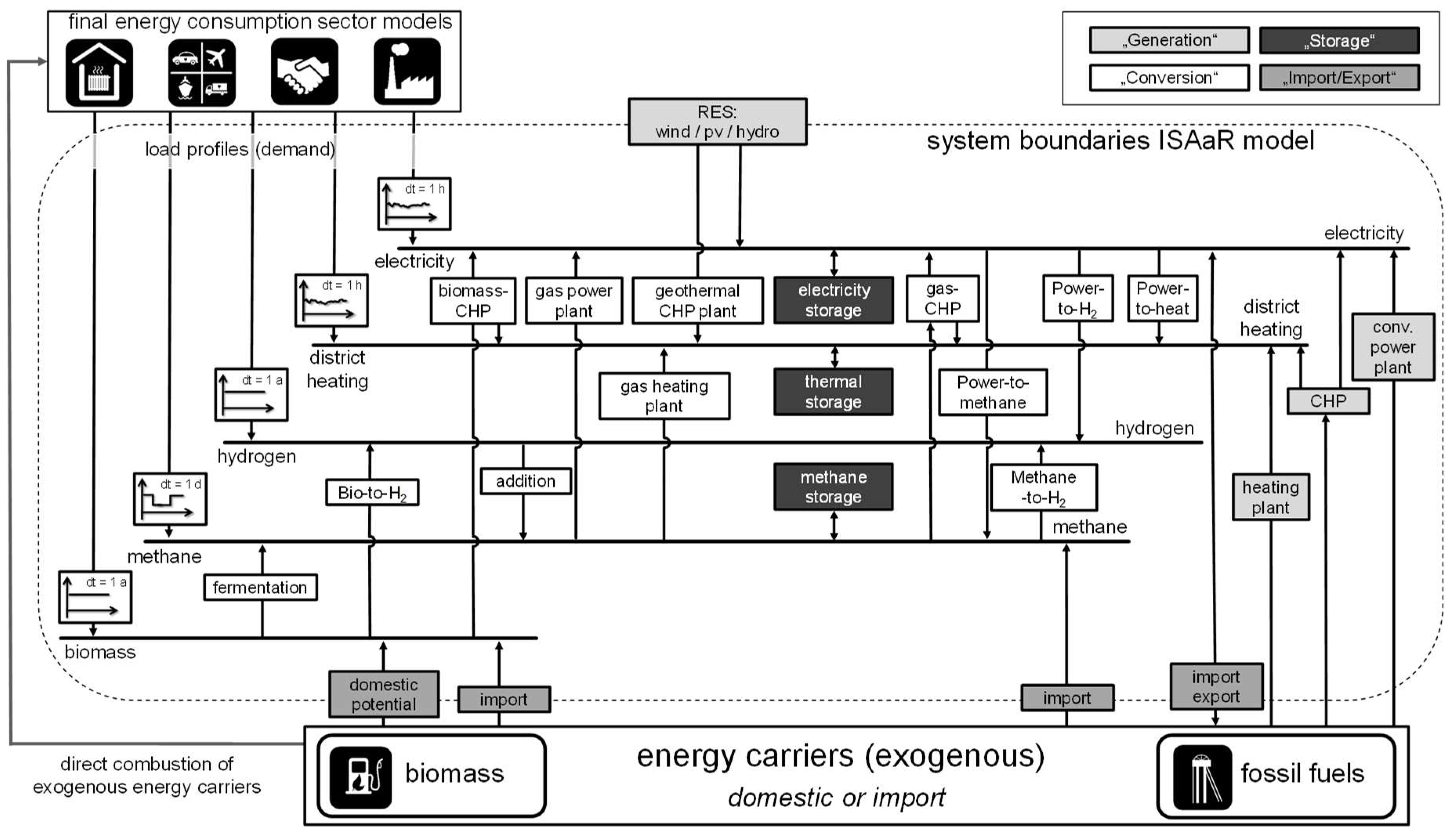
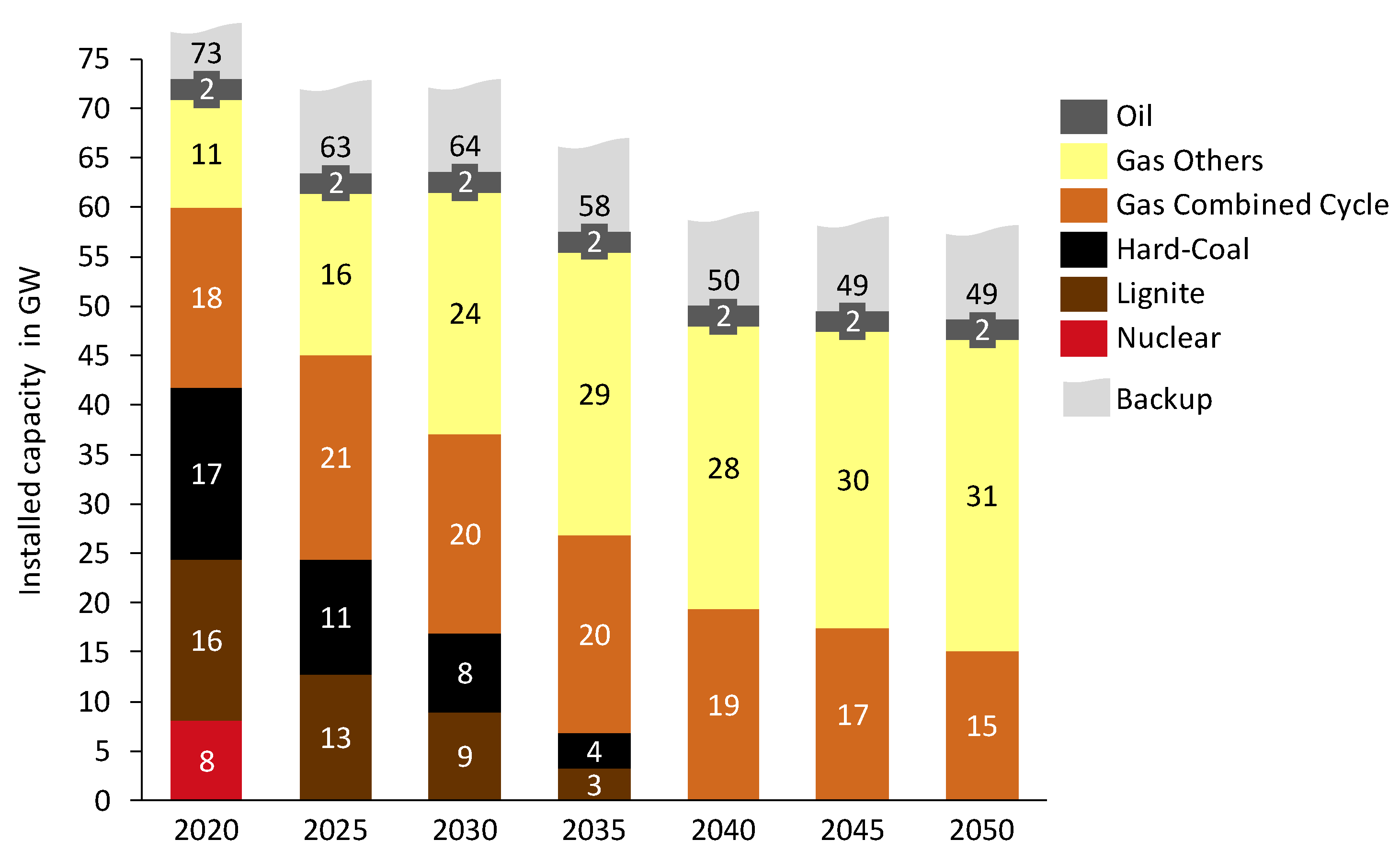
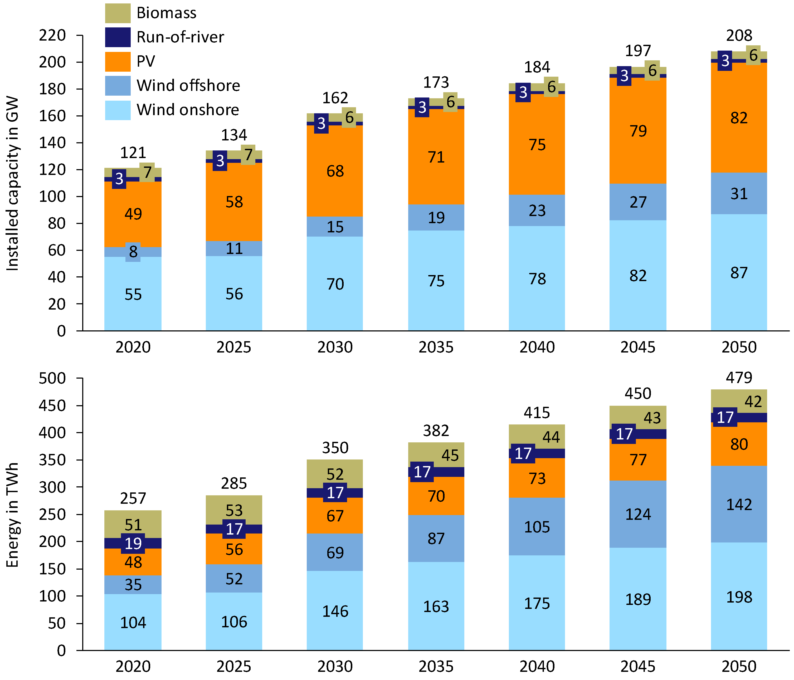
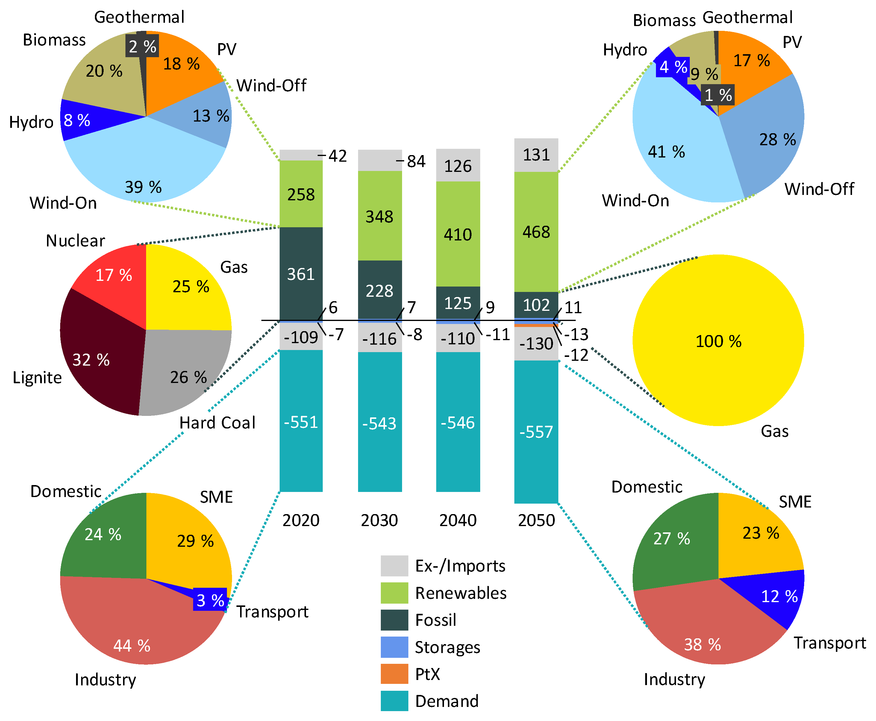
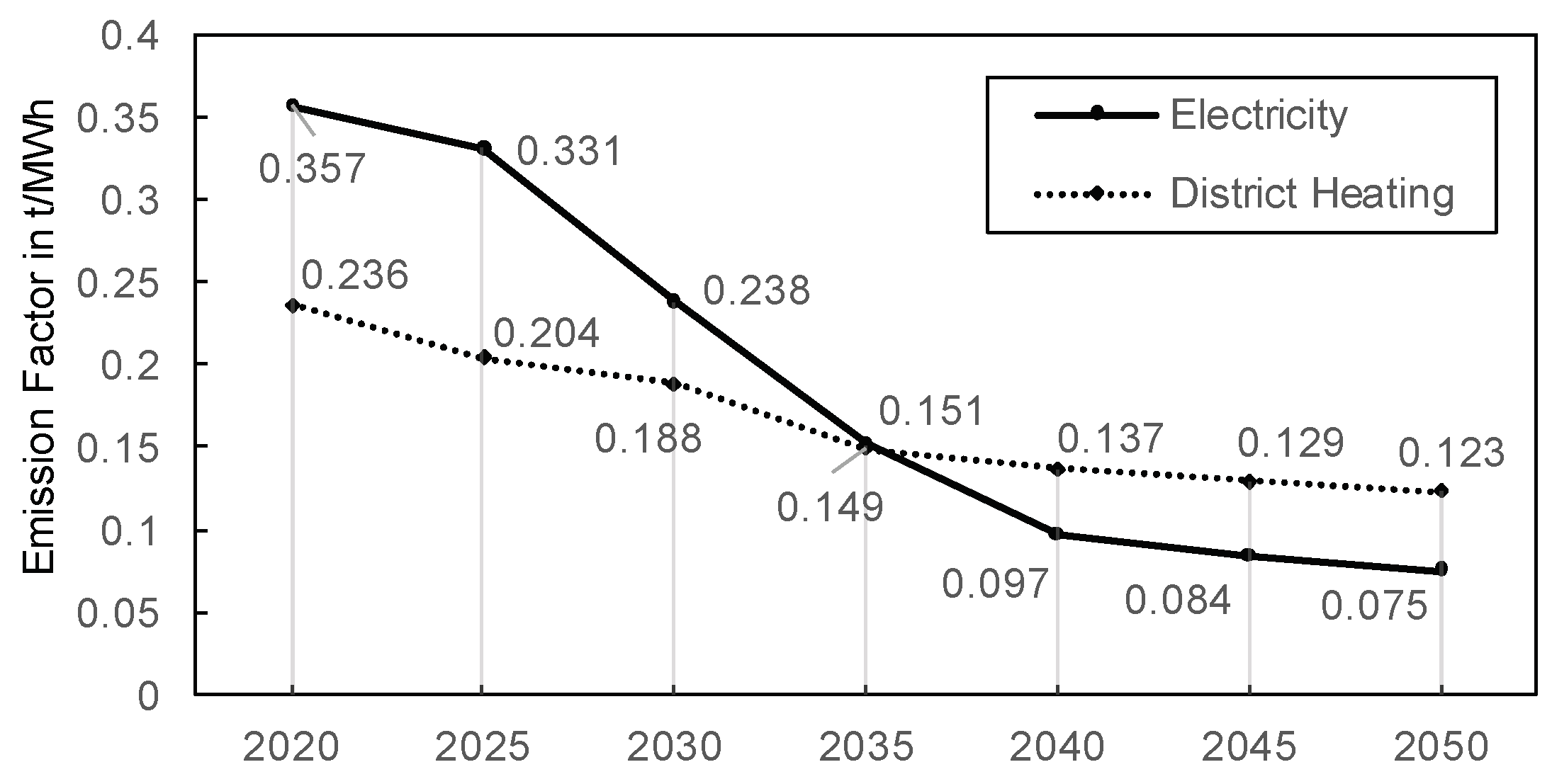
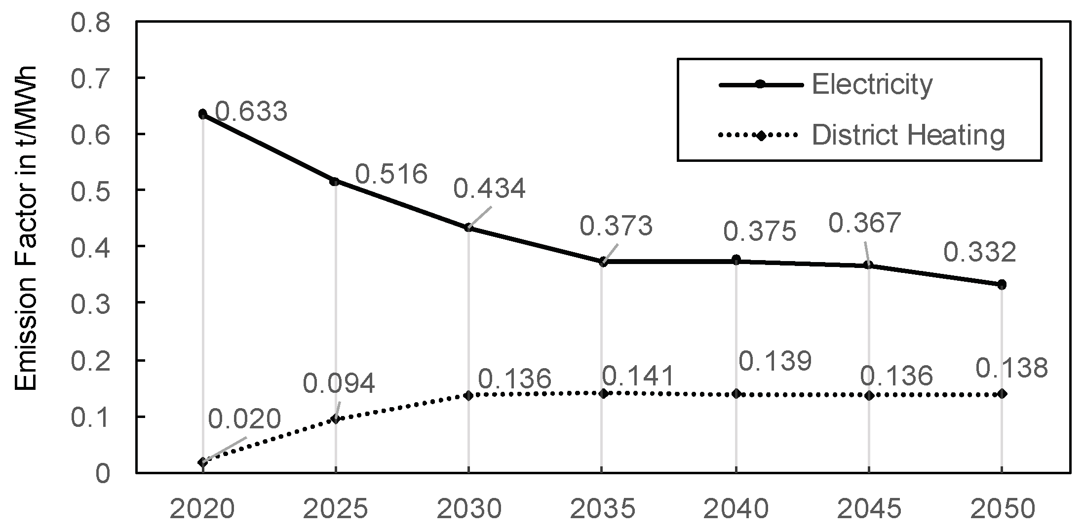
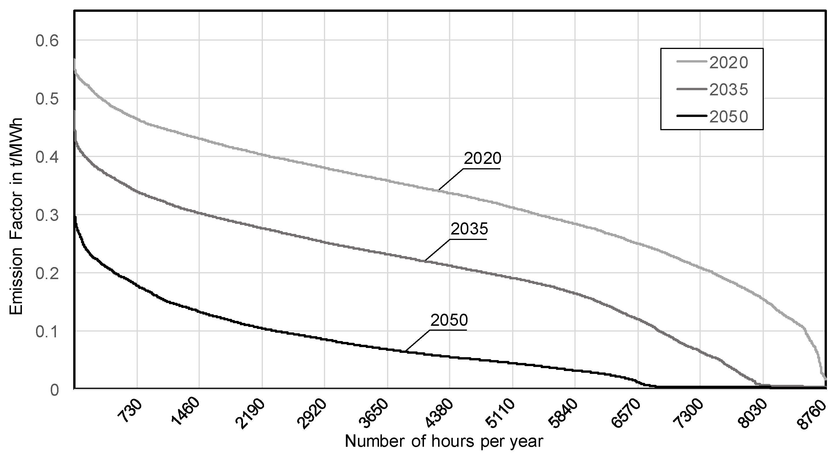
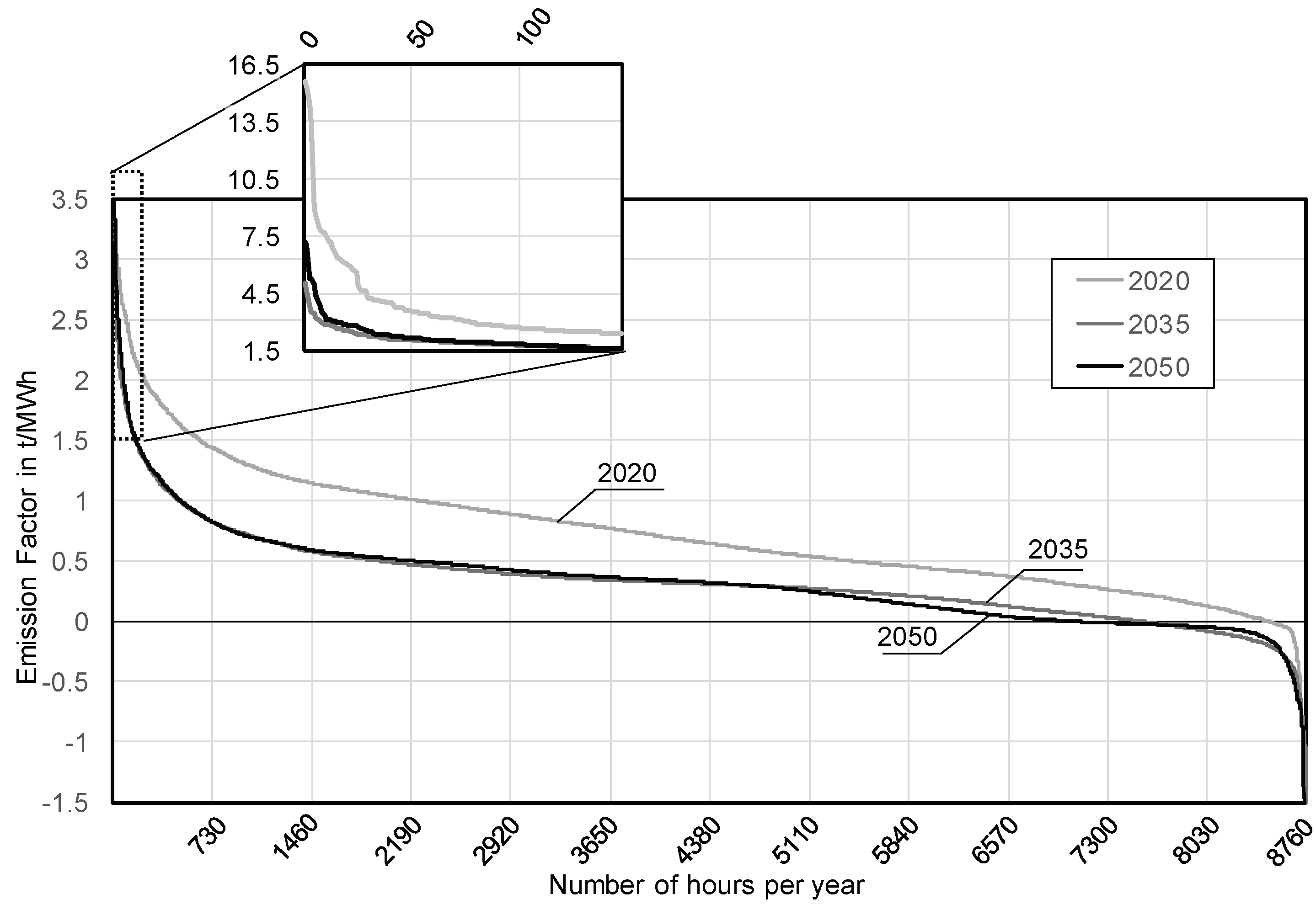
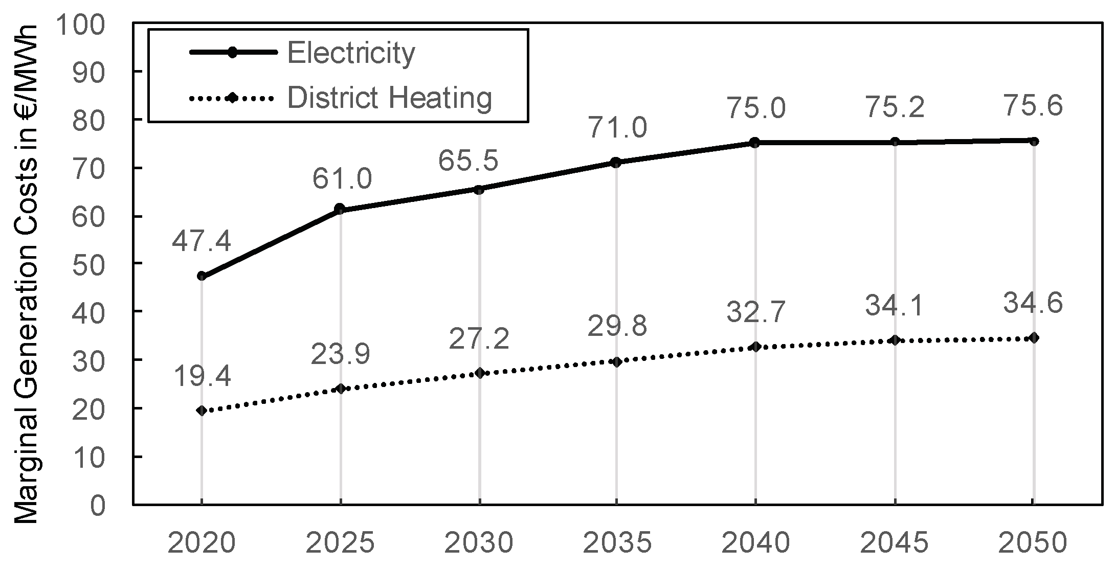
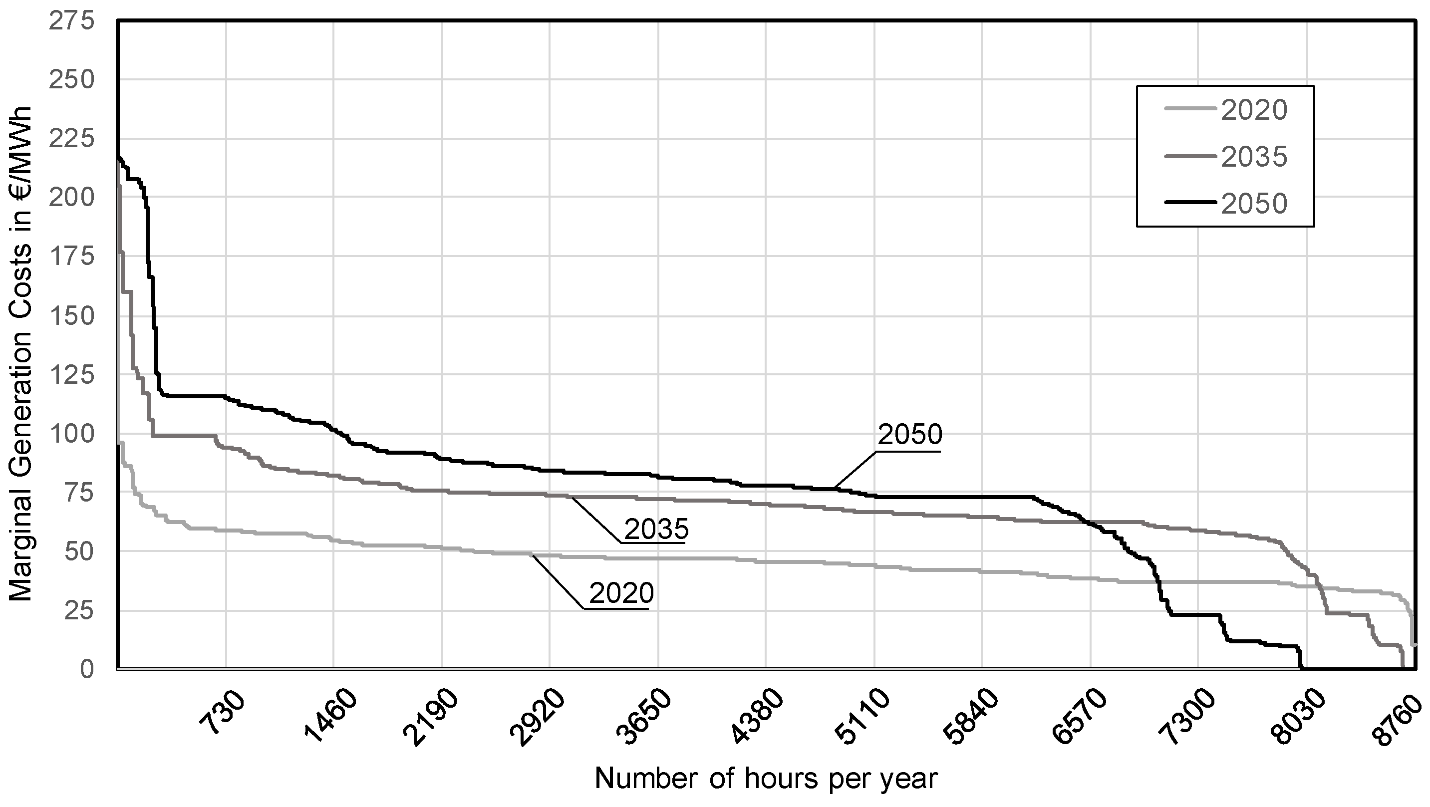
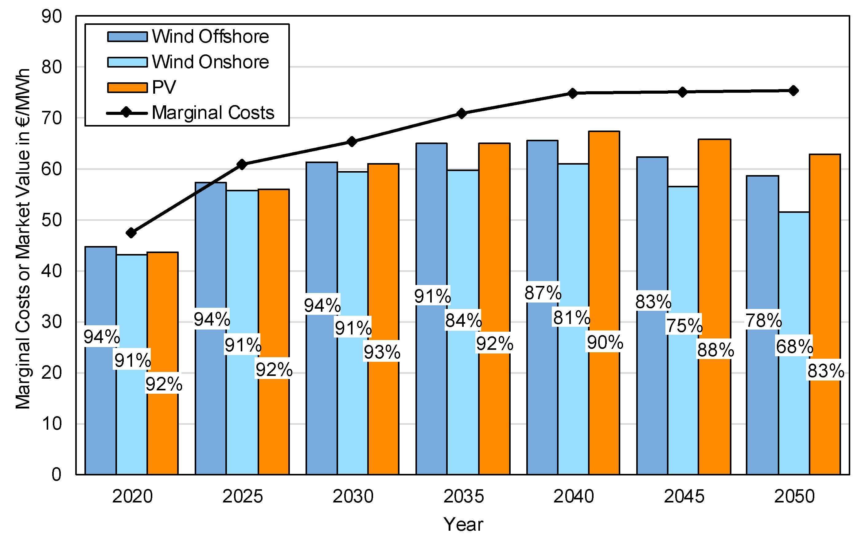
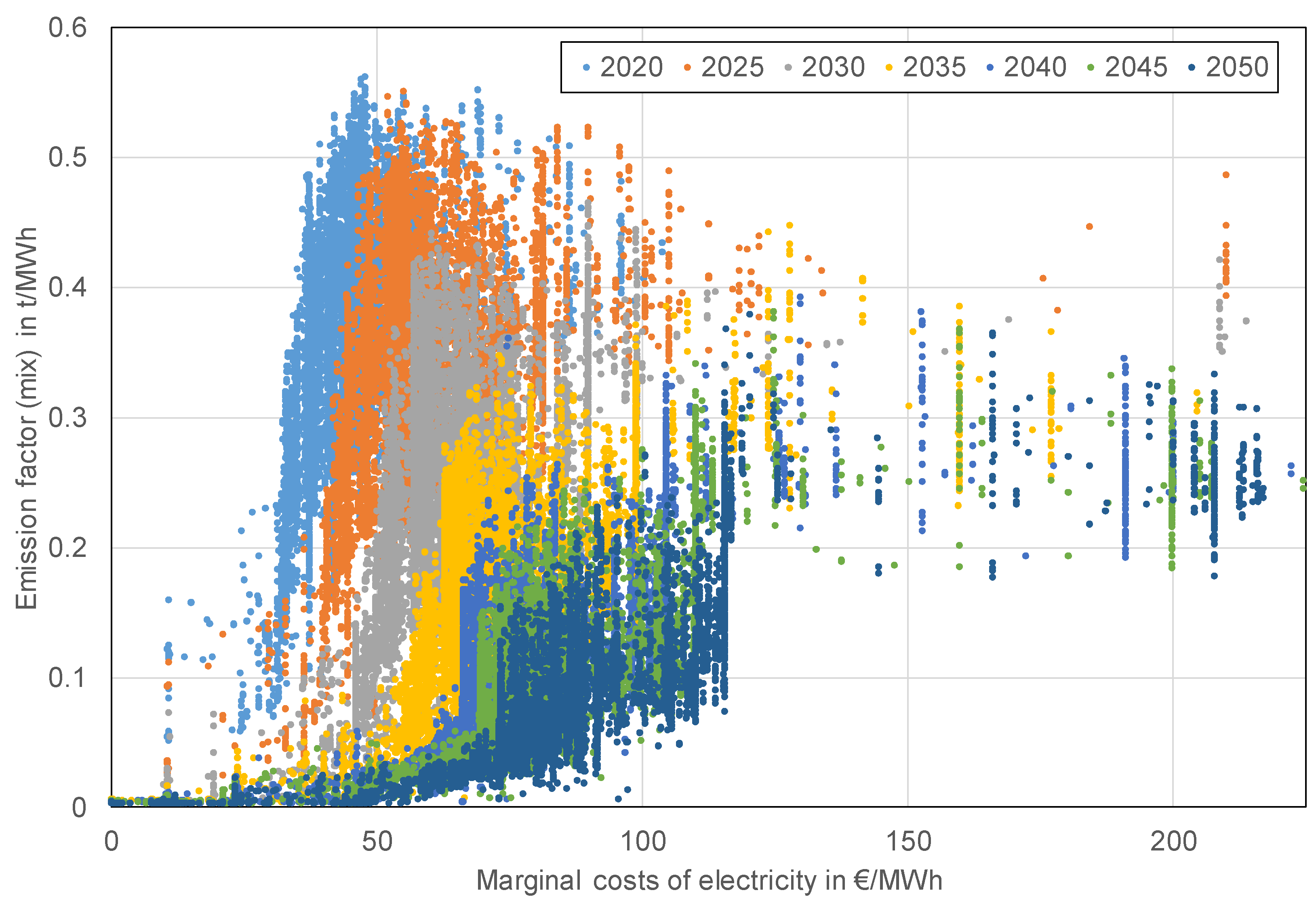
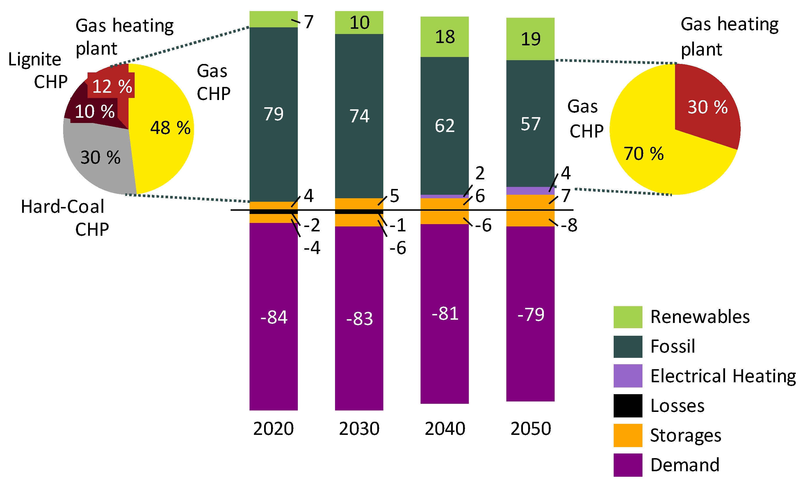
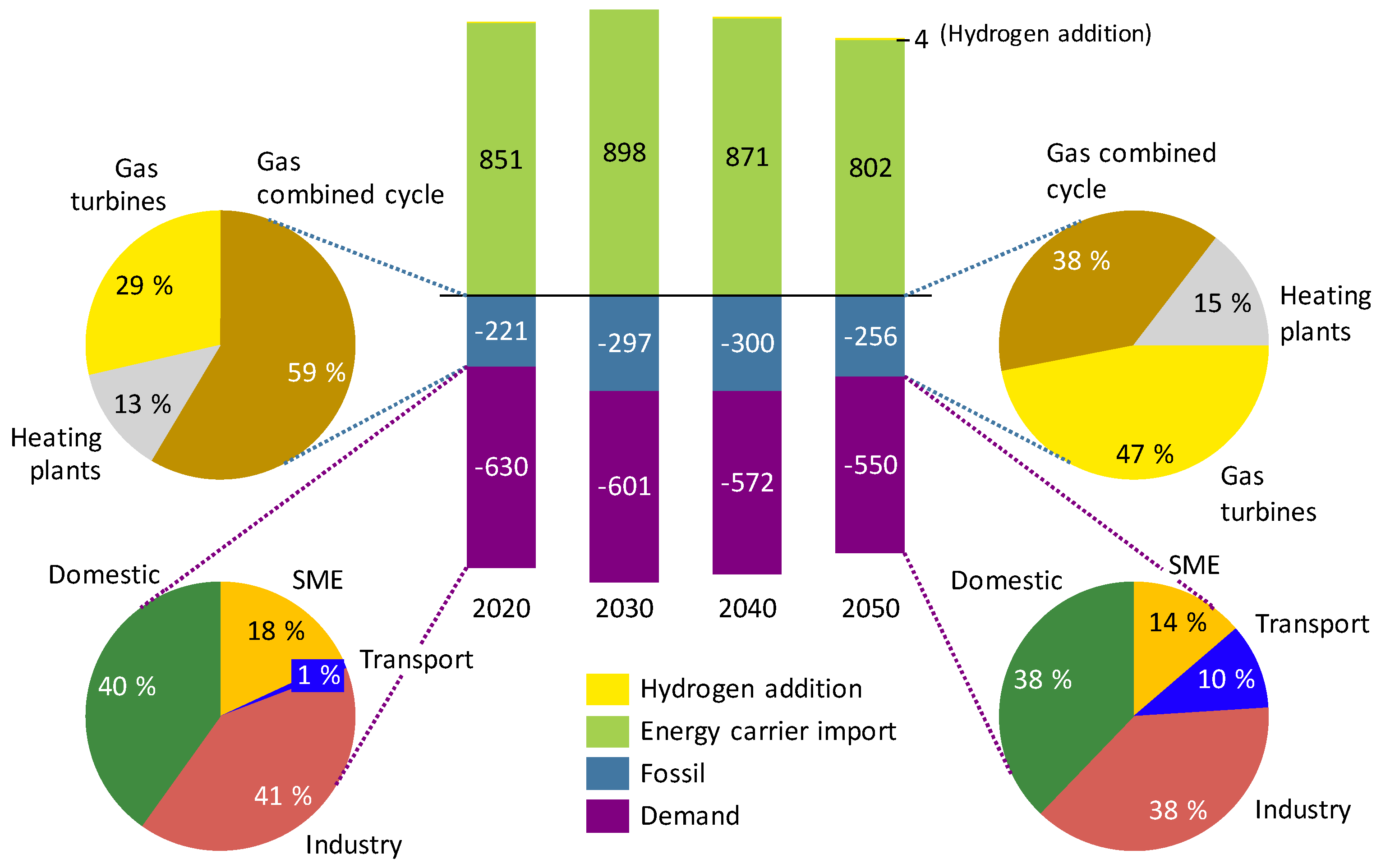
Table A1.
Costs (real) of fuels (net calorific value) and prices of CO2 certificates.
| Fuel: | Hard Coal | Lignite | Methane | Oil | Uranium | CO2 Price | |
|---|---|---|---|---|---|---|---|
| Unit: | €/MWh | €/MWh | €/MWh | €/MWh | €/MWh | €/t | |
| Costs: | 2015 | 8.3 | 3.0 | 20.2 | 30.1 | 3.6 | 5.4 |
| 2020 | 8.4 | 4.3 | 22.7 | 40.0 | 3.3 | 20.1 | |
| 2025 | 8.5 | 5.6 | 25.2 | 49.9 | 3.3 | 31.0 | |
| 2030 | 8.4 | 5.6 | 26.4 | 48.3 | 3.3 | 41.8 | |
| 2035 | 8.5 | 5.6 | 27.9 | 53.0 | 3.3 | 52.7 | |
| 2040 | 8.9 | 5.6 | 28.0 | 53.0 | 3.3 | 63.5 | |
| 2045 | 9.3 | 5.6 | 28.0 | 53.0 | 3.3 | 74.4 | |
| 2050 | 9.8 | 5.6 | 28.1 | 53.0 | 3.3 | 85.2 | |
The direct CO2 emissions resulting from the combustion of fuels, are determined based on stoichiometry for methane and from the national greenhouse gas inventory report [75] for all other fuels. Table A2 gives an overview of the resulting emission factors of fuels.
Table A2.
Direct CO2 emission factors of fuels (net calorific value).
| Fuel: | Hard Coal | Lignite | Oil | Methane |
|---|---|---|---|---|
| Unit: | t/MWh | t/MWh | t/MWh | t/MWh |
| Emission factor: | 0.337 | 0.399 | 0.264 | 0.199 |
Appendix D
1. District Heating
Figure A1.
German energy carrier balance district heating in TWh.

2. Methane
Figure A2.
German energy carrier balance of methane in TWh.

References
- Mancarella, P.; Andersson, G.; Pecas-Lopes, J.A.; Bell, K.R.W. Modeling of integrated multi-energy systems: Drivers, requirements, and opportunities. In Proceedings of the Power Systems Computation Conference (PSCC), Genua, Italy, 20–24 June 2016; IEEE: New York, NY, USA, 2016. [Google Scholar] [CrossRef]
- Bründlinger, T.; König, J.E.; Frank, O.; Gründig, D.; Jugel, C.; Kraft, P.; Krieger, O.; Mischinger, S.; Prein, P.; Seidl, H.; et al. Dena-Leitstudie Integrierte Energiewende—Impulse für die Gestaltung des Energiesystems bis 2050; Deutsche Energie-Agentur GmbH (dena), ewi Energy Research & Scenarios gGmbH: Berlin/Köln, Germany, 2018. [Google Scholar]
- Günther, J.; Lehmann, H.; Lorenz, U.; Purr, K. Den Weg zu Einem Treibhausgasneutrale Deutschland Ressourcenschonend Gestalten; Umweltbundesamt: Dessau-Roßlau, Germany, 2017. [Google Scholar]
- Gebert, P.; Herhold, P.; Burchardt, J.; Schönberger, S.; Rechenmacher, F.; Kirchner, A.; Kemmler, A.; Wünsch, M. Klimapfade für Deutschland, Studie im Auftrag des Bundesverbandes der Deutschen Industrie e.V. (BDI); The Boston Consultung Group und Prognos: München/Berlin, Germany, 2018. [Google Scholar]
- Pfluger, B.; Tersteegen, B.; Franke, B. Langfristszenarien für die Transformation des Energiesystems in Deutschland, Studie im Auftrag des Bundesministeriums für Wirtschaft und Energie (BMWi); Fraunhofer Institut für System- und Innovationsforschung (ISI): Karlsruhe, Germany; Consentec GmbH: Aachen, Germany; Insitut für Energie- und Umweltforschung GmbH (ifeu): Heidelberg, Germany, 2017. [Google Scholar]
- Capros, P.; Höglund-Isaksson, L.; Frank, S.; Witzke, H.P. EU Reference Scenario 2016; European Commission: Brussles, Belgium, 2016. [Google Scholar]
- Ryan, N.A.; Johnson, J.X.; Keoleian, G.A. Comparative assessment of models and methods to calculate grid electricity emissions. Environ. Sci. Technol. 2016, 50, 8937–8953. [Google Scholar] [CrossRef] [PubMed]
- Ripp, C.; Steinke, F. A first shot at time-dependent CO2 intensities in multi-modal energy systems. In Proceedings of the 15th International Conference on the European Energy Market (EEM), Lodz, Poland, 27–29 June 2018; IEEE: New York, NY, USA, 2018. [Google Scholar] [CrossRef]
- Regett, A.; Böing, F.; Conrad, J. Emission assessment of electricity: Mix vs. marginal power plant method. In Proceedings of the 15th International Conference on the European Energy Market (EEM), Lodz, Poland, 27–29 June 2018; IEEE: New York, NY, USA, 2018. [Google Scholar] [CrossRef]
- Böing, F.; Murmann, A.; Guminski, A. Electrification and coal phase-out in Germany: A scenario analysis. In Proceedings of the 15th International Conference on the European Energy Market (EEM), Lodz, Poland, 27–29 June 2018; IEEE: New York, NY, USA, 2018. [Google Scholar] [CrossRef]
- Böing, F.; Bruckmeier, A.; Murmann, A.; Pellinger, C.; Kern, T. Relieving the German transmission grid with regulated wind power development. In Proceedings of the 15th IAEE European Conference, Vienna, Austria, 3–6 September 2017; IAEE: Cleveland, OH, USA, 2017. [Google Scholar]
- Guminski, A.; Böing, F.; Murmann, A.; Roon, S. System effects of high demand-side electrification rates: A scenario analysis for Germany in 2030. WIREs Energy Environ. 2019, 8, e327. [Google Scholar] [CrossRef]
- Böing, F.; Murmann, A.; Pellinger, C.; Bruckmeier, A.; Kern, T.; Mongin, T. Assessment of grid optimisation measures for the German transmission grid using open source grid data. J. Phys. Conf. Ser. 2018, 977, 012002. [Google Scholar] [CrossRef]
- Pellinger, C.; Schmid, T. Merit Order der Energiespeicherung im Jahr 2030—Hauptbericht; Forschungsstelle für Energiewirtschaft (FfE): München, Germany, 2016. [Google Scholar]
- Pellinger, C. Mehrwert Funktionaler Energiespeicher aus System- und Akteurssicht. Ph.D. Thesis, Technical University Munich, Munich, Germany, July 2016. [Google Scholar]
- Boyd, S.; Vandenberghe, L. Convex Optimization; Cambridge University Press: Cambridge, UK, 2004. [Google Scholar]
- Bazaraa, M.S.; Jarvis, J.J.; Sherali, H.D. Linear Programming and Network Flows; John Wiley & Sons Inc.: Hoboken, NJ, USA, 2009. [Google Scholar] [CrossRef]
- Netzentwicklungsplan Strom. Szenariorahmen für den Netzentwicklungsplan Strom 2030 (Version 2019)—Entwurf der Übertragungsnetzbetreiber; 50Hertz Transmission GmbH: Berlin, Germany; Amprion GmbH: Dortmund, Germany; TenneT TSO GmbH: Bayreuth, Germany; TransnetBW GmbH: Stuttgart, Germany, 2018. [Google Scholar]
- Weber, C. Uncertainty in the Electric Power Industry; Springer: Berlin, Germany, 2005. [Google Scholar] [CrossRef]
- Müller-Syring, G.; Henel, M.; Köppel, W.; Mlaker, H.; Sterner, M.; Höcher, T. Entwicklung von Modularen Konzepten zur Erzeugung, Speicherung und Einspeisung von Wasserstoff und Synthetischem Methan in das Erdgasnetz, Studie im Auftrag der DVGW; DBI Gas- und Umwelttechnik GmbH: Leipzig, Germany; DVGW: Bonn, Germany; E.ON: Essen, Germany; Fraunhofer IWES: Kassel, Germany, 2013. [Google Scholar]
- Fishbone, L.; Abilock, H. Markal, a linear-programming model for energy systems analysis: Technical description of the Bnl version. Int. J. Energy Res. 1981, 5, 353–375. [Google Scholar] [CrossRef]
- ENTSO-E. TYNDP—Ten Year Net Developing Plan; ENTSO-E: Brussles, Belgium, 2018; Available online: http://tyndp.entsoe.eu/maps-data/ (accessed on 4 February 2019).
- Schlesinger, M.; Lindenberger, D.; Lutz, C. Entwicklung der Energiemärkte—Energiereferenzprognose, Studie im Bundesministeriums für Wirtschaft und Technologie (BMWi); BMWi: Berlin, Germany, 2014. [Google Scholar]
- Federal Ministry for Economic Affairs and Energy (BMWi). Final Report: Commission on Growth, Structural Change and Employment; Federal Ministry for Economic Affairs and Energy (BMWi): Berlin, Germany, 2018; Available online: https://www.bmwi.de/Redaktion/EN/Publikationen/commission-on-growth-structural-change-and-employment.pdf?__blob=publicationFile&v=3 (accessed on 4 February 2019).
- Platts. WEPP Database (Europe); Platts: Washington, DC, USA, 2018. [Google Scholar]
- Bundesnetzagentur für Elektrizität, Gas, Telekommunikation, Post und Eisenbahnen (BNetzA). Kraftwerksliste der Bundesnetzagentur—Stand November 2018; Bundesnetzagentur für Elektrizität, Gas, Telekommunikation, Post und Eisenbahnen (BNetzA): Bonn, Germany, 2018; Available online: https://www.bundesnetzagentur.de/DE/Sachgebiete/ElektrizitaetundGas/Unternehmen_Institutionen/Versorgungssicherheit/Erzeugungskapazitaeten/Kraftwerksliste/kraftwerksliste-node.html (accessed on 13 December 2018).
- Bundesnetzagentur für Elektrizität, Gas, Telekommunikation, Post und Eisenbahnen (BNetzA). Veröffentlichung Zu- und Rückbau—Kraftwerksliste der Bundesnetzagentur—Stand November 2018; Bundesnetzagentur für Elektrizität, Gas, Telekommunikation, Post und Eisenbahnen (BNetzA): Bonn, Germany, 2018; Available online: https://www.bundesnetzagentur.de/DE/Sachgebiete/ ElektrizitaetundGas/Unternehmen_Institutionen/Versorgungssicherheit/Erzeugungskapazitaeten/Kraftwerksliste/kraftwerksliste-node.html (accessed on 13 December 2018).
- Umweltbundesamt (UBA). Kraftwerke in Deutschland (ab 100 Megawatt elektrischer Leistung); Umweltbundesamt (UBA): Dessau-Roßlau, Germany, 2018; Available online: https://www.umweltbundesamt.de/dokument/datenbank-kraftwerke-in-deutschland (accessed on 13 December 2018).
- Von Roon, S.; Dossow, P.; Kern, T.; Hinterstocker, M.; Pellinger, C. Relevance and chances for industrial self-generation of electricity for high market shares of renewable energies. In Proceedings of the 11th Internationale Energiewirtschaftstagung an der TU Wien, Vienna, Austria, 13–15 February 2019; Available online: https://iewt2019.eeg.tuwien.ac.at/download/contribution/fullpaper/261/261_fullpaper_20190218_225307.pdf (accessed on 23 April 2019).
- Schluss-be-Richt. Langfristszenarien und Strategien für den Ausbau der Erneuerbaren Energien in Deutschland bei Berücksichtigung der Entwicklung in Europa und global Datenanhang II zum Schlussbericht, Studie im Auftrag des Bundesministeriums für Umwelt, Naturschutz und Reaktorsicherheit; Fraunhofer-Institut für Windenergie und Energiesystemtechnik (IWES): Stuttgart, Germany; Ingenieurbüro für neue Energien (IfnE): Kassel, Germany; Deutsches Zentrum für Luft- und Raumfahrt e. V. (DLR): Teltow, Germany, 2012; Available online: https://www.dlr.de/tt/Portaldata/41/Resources/dokumente/institut/system/publications/Leitstudie_2011_-_Tabellen_Datenanhang_II.xls (accessed on 23 April 2019).
- Henning, H.-M.; Palzer, A. Was kostet die Energiewende?—Wege zur Transformation des deutschen Energiesystems bis 2050; Fraunhofer Institut für Solare Energiesystem (ISE): Freiburg, Germany, 2015; Available online: https://www.fraunhofer.de/content/dam/zv/de/Forschungsfelder/Energie-Rohstoffe/Fraunhofer-ISE_Transformation-Energiesystem-Deutschland_final_19_11%20(1).pdf (accessed on 4 June 2014).
- ASUE. BHKW-Kenndaten 2014/2015—Module, Anbieter, Kosten; Arbeitsgemeinschaft für Sparsamen und Umweltfreundlichen Energieverbrauch e.V. (ASUE): Berlin, Germany, 2014. [Google Scholar]
- Kesicki, F.; Ekins, P. Marginal abatement cost curves: A call for caution. Clim. Policy 2012, 12, 219–236. [Google Scholar] [CrossRef]
- Schroedter-Homscheidt, M.; Hoyer-Klick, C.; Killius, N.; Lefèvre, M.; Wald, L.; Wey, E.; Saboret, L. User’s Guide to the CAMS Radiation Service—Status December 2016; ECMWF: Shinfield Park, Reading, UK, 2016. [Google Scholar]
- Schulz, J.-P.; Schättler, U. Beschreibung des Lokal-Modells Europa COSMO-EU (LME) und seiner Datenbanken auf dem Datenserver des DWD; Deutscher Wetterdienst (DWD): Offenbach, Germany, 2011. [Google Scholar]
- Müller, M.; Reinhard, J.; Ostermann, A.; Estermann, T.; Köppl, S. Regionales flexibilitäts-potenzial dezentraler anlagen—modellierung und bewertung des regionalen flexibilitäts-potenzials von dezentralen flexibilitäts-typen im verteilnetz. In Proceedings of the Konferenzband der Konferenz Zukünftige Stromnetze, Berlin, Germany, 30–31 Januar 2019; Connexio GmbH: Pforzheim, Germany, 2019. [Google Scholar]
- Figgener, J.; Haberschusz, D.; Kairies, K.-P.; Tepe, B.; Ebbert, M.; Herzog, R.; Sauer, D.U. Wissenschaftliches Mess- und Evaluierungsprogramm Solarstromspeicher 2.0—Jahresbericht 2017; Institut für Stromrichtertechnik und Elektrische Antriebe der RWTH Aachen: Aachen, Germany, 2017. [Google Scholar]
- Bundesnetzagentur für Elektrizität, Gas, Telekommunikation, Post und Eisenbahnen (BnetzA). Genehmigung des Szenariorahmens für die Netzentwicklungsplanung 2019–2030; Bundesnetzagentur für Elektrizität, Gas, Telekommunikation, Post und Eisenbahnen (BNetzA): Bonn, Germany, 2018. [Google Scholar]
- Hecker, C.; Zauner, E.; Pellinger, C.; Carr, L.; Hötzl, S. Modellierung der flexiblen Energiebereitstellung von Wasserkraftwerken in Europa. In Proceedings of the Konferenzband der 17th Internationale Energiewirtschaftstagung an der TU Wien, Vienna, Austria, 15–17 February 2015; AAEE: Sycamore, IL, USA, 2015. [Google Scholar]
- ENTSO-E. Net Transfer Capacity (NTC) and Available Transfer Capacities (ATC) in the Internal Market of Electricity in Europe (IEM); ENTSO-E: Brussles, Belgium, 2000; Available online: https://www.entsoe.eu/fileadmin/user_upload/_library/ntc/entsoe_NTCusersInformation.pdf (accessed on 24 April 2019).
- ENTSO-E. Transparency Plattform; ENTSO-E: Brussles, Belgium, 2016; Available online: https://transparency.entsoe.eu (accessed on 20 March 2016).
- Conrad, J.; Greif, S. Modeling the Private Households Sector and the Impact on the Energy System. In Proceedings of the 41st IAEE Conference, Groningen, The Netherlands, 10–13 June 2018; IAEE: Cleveland, OH, USA, 2018. [Google Scholar]
- Conrad, J.; Greif, S. Modeling load profiles of heat pumps. Energies 2019, 12, 766. [Google Scholar] [CrossRef]
- Pichlmaier, S.; Bayer, C. Modelling the transport sector in the context of a dynamic energy system. In Proceedings of the 41st IAEE Conference, Groningen, The Netherlands, 10–13 June 2018; IAEE: Cleveland, OH, USA, 2018. [Google Scholar]
- Öffentliche Nettostromerzeugung in Deutschland—Erneuerbare Energiequellen erreichen über 40 Prozent, Pressemitteilung des Fraunhofer ISE. Available online: https://www.ise.fraunhofer.de/de/presse-und-medien/news/2018/nettostromerzeugung-2018.html (accessed on 9 January 2019).
- AGFW. AGFW—Hauptbericht 2016; AGFW: Frankfurt am Main, Germany, 2017; Available online: https://www.agfw.de/index.php?eID=tx_securedownloads&p=436&u=0&g=0&t=1556182285&hash=3253fea8235754ef2787f657b4379ea4260cf62f&file=fileadmin/user_upload/Zahlen_und_Statistiken/Version_1_HB2016.pdf (accessed on 24 April 2019).
- Conrad, J.; Greif, S.; Kleinertz, B.; Pellinger, C. Flexibilisierung der Kraft-Wärme- Kopplung—Kurzgutachten im Auftrag der Übertragungsnetzbetreiber in Deutschland; Forschungsstelle für Energiewirtschaft e.V. (FfE): München, Germany, 2017; Available online: https://www.ffe.de/attachments/article/761/Flexibilisierung%20der%20Kraft-Waerme-Kopplung.pdf (accessed on 24 April 2019).
- BAFA. Zulassung von KWK-Anlagen nach dem Kraft-Wärme-Kopplungsgesetz (KWKG); Bundesamt für Wirtschaft und Ausfuhrkontrolle (BAFA): Eschborn, Germany, 2014. [Google Scholar]
- Kail, C.; Spahn, K.; Grupczynski, M. Die Brennstoff-Frage—Energieversorgungslösungen für Industrie und Kommunen. BWK 2010, 62, 58–66. [Google Scholar]
- Kail, C.; Haberberger, G. Kenngrößen zur optimalen Auslegung großer KWK-Anlagen. VDI-Berichte 2001, 1594, 99–112. [Google Scholar]
- Pehnt, M. Energieeffizienz—Ein Lehr- und Handbuch; Springer: Berlin, Germany, 2010. [Google Scholar] [CrossRef]
- Estermann, T.; Pichlmaier, S.; Guminski, A.; Pellinger, C. Kurzstudie Power-to-X—Ermittlung des Potenzials von PtX-Anwendungen im Auftrag der Übertragungsnetzbetreiber in Deutschland; Forschungsstelle für Energiewirtschaft e.V. (FfE): München, Germany, 2017; Available online: https://www.ffe.de/attachments/article/761/Kurzstudie%20Power-to-X.pdf (accessed on 24 April 2019).
- Kern, T.; Buchwitz, K.; Guminski, A.; von Roon, S. The impact of electrification on the gas sector. In Proceedings of the 15th International Conference on the European Energy Market (EEM), Lodz, Poland, 27–29 June 2018; IEEE: New York, NY, USA, 2018. [Google Scholar] [CrossRef]
- Kern, T.; Eberl, B.; Böing, F.; von Roon, S. Coupling of electricity and gas market models. In Proceedings of the 14th International Conference on the European Energy Market (EEM), Dresden, Germany, 6–9 June 2017; IEEE: New York, NY, USA, 2017. [Google Scholar] [CrossRef]
- ENTSO-G Transmission Capacity Map. Available online: https://www.entsog.eu/maps/transmission-capacity-map (accessed on 1 April 2018).
- AGSI+ Transparency Plattform. Available online: https://agsi.gie.eu/ (accessed on 5 June 2018).
- Heijungs, R.; Suh, S. The Computational Structure of Life Cycle Assessment; Springer: Amsterdam, The Netherlands, 2002. [Google Scholar] [CrossRef]
- Tereshchenko, T.; Nord, N. Uncertainty of the allocation factors of heat and electricity production of combined cycle power plant. Appl. Therm. Eng. 2015, 76, 410–422. [Google Scholar] [CrossRef] [Green Version]
- IEA Sankey Diagramm. Available online: https://www.iea.org/Sankey/#?c=Germany&s=Balance (accessed on 24 April 2019).
- Tranberg, B.; Corradi, O.; Lajoie, B.; Gibon, T.; Staffell, I.; Andresen, G.B. Real-time carbon accounting method for the European electricity markets. In Energy Strategy Reviews; Howells, M., Ed.; Elsevier: Amsterdam, The Netherlands, 2019; Available online: https://arxiv.org/abs/1812.06679 (accessed on 23 April 2019).
- Kleinertz, B.; Pellinger, C.; von Roon, S.; Hübner, T.; Kaestle, G. EU Displacement Mix—A Simplified Marginal Method to Determine Environmental Factors for Technologies Coupling Heat and Power in the European Union; Forschungsstelle für Energiewirtschaft (FfE): Munich, Germany, 2018. [Google Scholar]
- Schweppe, F.C.; Caramanis, M.C.; Tabors, R.D.; Bohn, R.E. Spot Pricing of Electricity; Springer: New York, NY, USA, 1988. [Google Scholar] [CrossRef]
- Müsgens, F. Quantifying market power in the german wholesale electricity market using a dynamic multi-regional dispatch model. J. Ind. Econ. 2006, 54, 471–498. [Google Scholar] [CrossRef]
- Mann, N.; Tsai, C.-H.; Gülen, G.; Schneider, E.; Chuevas, P.; Dyer, J.; Butler, J.; Zhang, T.; Baldick, R.; Deetjen, T.; et al. Capacity Expansion and Dispatch Modeling: Model Documentation and Results for ERCOT Scenarios; The University of Texas at Austin: Austin, TX, USA, 2017; Available online: https://energy.utexas.edu/sites/default/files/UTAustin_FCe_ERCOT_2017.pdf (accessed on 24 April 2019).
- Umweltbundesamt (UBA). Submission under the United Nations Framework Convention on Climate Change and the Kyoto Protocol 2016—National Inventory Report for the German Greenhouse Gas Inventory 1990–2014; Umweltbundesamt (UBA): Dessau-Roßlau, Germany, 2016. [Google Scholar]
- Burger, B. Stromerzeugung in Deutschland im Jahr 2016; Fraunhofer-Institut für Solare Energiesysteme (ISE): Freiburg, Germany, 2017; Available online: https://www.ise.fraunhofer.de/content/dam/ise/de/documents/publications/studies/Stromerzeugung_2016.pdf (accessed on 24 April 2019).
- Hirth, L. The market value of variable renewables. Energy Econ. 2013, 38, 218–236. [Google Scholar] [CrossRef] [Green Version]
- Phelix-DE Futures European Energy Exchange (EEX). Available online: https://www.eex.com/de/marktdaten/strom/futures/phelix-de-futures#!/2019/04/11 (accessed on 24 April 2019).
- Steurer, M.; Fahl, U.; Eberl, T.; Voß, A. Identifikation und Bewertung des intelligenten Lastmanagementpotenzials in der Industrie in Baden-Württemberg, Studie im Auftrag der EnBW Vertrieb GmbH; Institut für Energiewirtschaft und Rationelle Energieanwendung (IER): Stuttgart, Germany, 2013. [Google Scholar]
- Heilek, C. Modellgestützte Optimierung des Neubaus und Einsatzes von Erzeugungsanlagen und Speichern für elektrische und thermische Energie im deutschen Energiesystem. Ph.D.Thesis, Technical University Munich, Munich, Germany, March 2015. [Google Scholar]
- Bundesministerium für Wirtschaft und Energie (BMWi). Zahlen und Fakten Energiedaten 2016–Nationale und internationale Entwicklung; Bundesministerium für Wirtschaft und Energie (BMWi): Berlin, Germany, 2017. [Google Scholar]
- Bundesministerium für Wirtschaft und Energie (BMWi). Zahlen und Fakten Energiedaten 2017—Nationale und internationale Entwicklung; Bundesministerium für Wirtschaft und Energie (BMWi): Berlin, Germany, 2018. [Google Scholar]
- Industrie- und Handelskammer (IHK). Projektionsbericht 2017 für Deutschland—Gemäß Verordnung (EU) Nr. 525/2013; Industrie- und Handelskammer (IHK): Karlsruhe, Germany, 2017. [Google Scholar]
- Intercontinental Exchange (ICE). Market. Data; Intercontinental Exchange (ICE): Atlanta, GA, USA, 2017; Available online: https://www.theice.com/market-data (accessed on 10 September 2017).
- Energiewirtschaftliches Institut an der Universität zu Köln (EWI). Techno-ökonomische Kennwerte für den Forschungsverbund—Systemanalyse Energiespeicher; Energiewirtschaftliches Institut an der Universität zu Köln (EWI): Köln, Germany, 2014. [Google Scholar]
Figure 1.
Multi-energy carrier model “ISAaR”.

Figure 2.
Installed conventional generation capacities Germany (excluding back-up capacities).

Figure 3.
Installed variable renewable energy sources (vRES) and biomass capacities and yearly energy generation in Germany.
Figure 3.
Installed variable renewable energy sources (vRES) and biomass capacities and yearly energy generation in Germany.

Figure 4.
Resulting German energy balance for electricity in TWh.

Figure 5.
Emission factor of electricity (mix) in tons of CO2 per MWh; combined heat and power (CHP) allocation method: Carnot.
Figure 5.
Emission factor of electricity (mix) in tons of CO2 per MWh; combined heat and power (CHP) allocation method: Carnot.

Figure 6.
Emission factor of electricity and district heating (marginal) in tons of CO2 per MWh.

Figure 7.
Year duration line: hourly emission factor of electricity (mix) in tons of CO2 per MWh; CHP allocation method: Carnot.
Figure 7.
Year duration line: hourly emission factor of electricity (mix) in tons of CO2 per MWh; CHP allocation method: Carnot.

Figure 8.
Year duration line: hourly emission factor of electricity (marginal) in tons of CO2 per MWh in 2020, 2035, 2040.
Figure 8.
Year duration line: hourly emission factor of electricity (marginal) in tons of CO2 per MWh in 2020, 2035, 2040.

Figure 9.
Load weighted marginal costs of electricity and district heating generation in € per MWh.

Figure 10.
Year duration line: hourly marginal costs of electricity in € per MWh.

Figure 11.
Marginal costs of electricity and market value of vRES (wind and photovoltaic (PV)) in €/MWh.
Figure 11.
Marginal costs of electricity and market value of vRES (wind and photovoltaic (PV)) in €/MWh.

Figure 12.
Hourly emission factors of electricity (mix, Carnot) and marginal costs of electricity.

Table 1.
Selection and characterization of scenario sources.
| Source: | TYNDP 2018 1 | ERP 2 | NEP 2019 3 |
|---|---|---|---|
| Scenario Attributes ↓ Scenario Names → | “Sustainable Transition” | “Trend-Szenario” | “Szenario B” |
| Consistent representation of developments in neighboring European countries | yes | no | no |
| Sufficient level of detail for bottom-up modeling of German final energy consumption | no | yes | no |
| Scenario until 2050? | until 2040 | yes | until 2035 |
| Development of renewable energy capacities in the highest possible regional resolution | Countries/ENTSO-E-regions | Country (GER) | Federal States (GER) |
| High differentiation of electricity generation technologies | Yes | No | Yes |
| Detailed consideration of the German conventional power plant fleet | No | No | Yes |
1 TYNDP2018: Ten-Year Network Development Plan 2018 of ENTSO-E, publication: 2018 [22]. 2 ERP: “Energiereferenzprognose” (energy reference projection) publication: 2014 [23]. 3 NEP 2019: “Netzentwicklungsplan 2019” (German Network Development Plan 2019, Scenario framework draft), publication: 2018 [18].
© 2019 by the authors. Licensee MDPI, Basel, Switzerland. This article is an open access article distributed under the terms and conditions of the Creative Commons Attribution (CC BY) license (http://creativecommons.org/licenses/by/4.0/).
Share and Cite
MDPI and ACS Style
Böing, F.; Regett, A. Hourly CO2 Emission Factors and Marginal Costs of Energy Carriers in Future Multi-Energy Systems. Energies 2019, 12, 2260. https://doi.org/10.3390/en12122260
AMA Style
Böing F, Regett A. Hourly CO2 Emission Factors and Marginal Costs of Energy Carriers in Future Multi-Energy Systems. Energies. 2019; 12(12):2260. https://doi.org/10.3390/en12122260
Chicago/Turabian StyleBöing, Felix, and Anika Regett. 2019. "Hourly CO2 Emission Factors and Marginal Costs of Energy Carriers in Future Multi-Energy Systems" Energies 12, no. 12: 2260. https://doi.org/10.3390/en12122260
Note that from the first issue of 2016, this journal uses article numbers instead of page numbers. See further details here.