Accurate Expressions of Mutual Inductance and Their Calculation of Archimedean Spiral Coils

Abstract

Considering the helicity of Archimedean spiral coils, this paper proposes accurate expressions of mutual inductance and their numerical calculation methods, which can be applied in the wireless power transmission field, etc. Accurate expressions of mutual inductance are deduced respectively for two coils that are coaxial, laterally misaligned, or non-parallel, and numerical calculations are performed using Gaussian integration as well. In the case of coaxial coils, the calculation results are verified by the 3D finite element method (3D FEM) and compared with the results gained by the traditional method that approximates two spiral coils to two clusters of series-connected circular coils ignoring helicity. The comparison of the three methods shows that results achieved by the proposed expression are close to that of 3D FEM, while there is increasing error with the screw pitches of the coils when using the traditional circular coil approximation method. The influence of relative position on the mutual inductance of the two coils is also studied and it is further explained through magnetic field distribution. Finally, the validity of the proposed expressions of mutual inductance is verified by experimental results.

1. Introduction

Planar spiral coils have been widely used in high-frequency fields such as wireless power transmission [1,2], printed circuit board-based magnetic components, and on-chip coils [2,3]. In the design of the coils, mutual inductance is an important parameter [4,5]. Since Maxwell’s study, mutual inductance calculation has been considered as a basic scientific problem for all coupling coils [6]. The mutual inductance between circular filaments was first studied by Maxwell from the perspective of energy, and for the case of two coaxial coils, the mutual inductance expression containing a complete elliptic integral [7] was given. Based on the definition of mutual inductance in circuit theory and the concept of vector potential, Neumann’s formula of the mutual inductance between any two filaments was presented, and the mutual inductance between two parallel circular coils was calculated in [8,9]. By means of reciprocal distance under cylindrical coordinates, the variables in the mutual inductance expression of parallel circular coils was decoupled in [10]. The conclusion of [10] was applied in [3] to calculate the mutual inductance between coaxial coils considering the current distribution of the coils’ cross section. The mutual inductance of circular coils was studied in [11] and [12] under lateral misalignment and non-parallel occasions, respectively.

In industrial application fields like wireless power transmission, air core planar spiral coils with constant screw pitches, namely Archimedean spiral coils, are commonly used as the magnetic coupling mechanism [13,14]. In the calculation of the mutual inductance of planar spiral coils, the circular coils approximation method is commonly used in the existing literature. With this method, each of the two coils is approximately a cluster of concentric circular loops in series, and the total mutual inductance is the superposition of the mutual inductance of these loops [2,15,16,17], where the helicity of the coils is ignored. This approximation is reasonable when the coils’ screw pitches are far less than the radii, due to the destruction of axial symmetry not being evident. However, with regard to high-frequency magnetic coupling resonance wireless power transmission coils with a large transmission distance, the screw pitches are often large, which reduces the distributed capacitor and improves the Q value [18]. For helical coils, or namely solenoids, [19] figured out that helicity cannot be ignored at large pitch length, and mutual inductance between coaxial helical coils are presented analytically. Hence, the helicity of Archimedean spiral coils with large screw pitches should also be taken into account. However, unfortunately, there are few relevant studies on how helicity affects mutual inductance calculation results.

On the basis of Neumann’s formula [8] and the equation of the Archimedean spiral [1,13], accurate expressions of mutual inductance of Archimedean spiral coils applicable to arbitrary pitches are derived in this paper, and the corresponding numerical calculation methods are chosen as well. The double integral expressions of mutual inductance of a couple of Archimedean spiral coils at different relative positions are achieved with helicity taken into consideration, and these expressions are numerically solved by the Gaussian integral. When the two coils are coaxial, the calculation results are verified by the finite element software ANSYS Maxwell 3D simulation and compared with the traditional circular coils approximation method. The influence of the two coils’ relative position on mutual inductance is studied, and this is explained by magnetic field distribution analysis of a single current-carrying Archimedean spiral coil. Finally, a couple of Archimedean spiral coils are fabricated, and the experimental result verify the correctness of the analysis.

The paper is arranged as follows: Section 2 proposes the accurate expression of mutual inductance of a couple of coaxial Archimedean spiral coils, solves this expression numerically, and compares it with the traditional method; Section 3 proposes the accurate expression of mutual inductance of a couple of Archimedean spiral coils with lateral misalignment and studies the influence of distance and lateral misalignment on mutual inductance; Section 4 proposes the accurate expression of mutual inductance of a couple of Archimedean spiral coils with arbitrary relative position and studies the influence of angular misalignment on mutual inductance; Section 5 depicts the magnetic field distribution of an Archimedean spiral coil to explain the influence of relative position on mutual inductance; and Section 6 is the experimental verification.

2. Mutual Inductance between a Couple of Coaxial Archimedean Spiral Coils

2.1. Accurate Expression of Mutual Inductance of Coaxial Archimedean Spiral Coil

The mutual inductance between any coils C₁ and C₂ can be expressed by Neumann’s formula [8,9]:

$$M=\frac{{\mu }_0}{4\mathsf{\pi }}{\displaystyle \underset{{\mathrm{C}}_1}{\int }{\displaystyle \underset{{\mathrm{C}}_2}{\int }\frac{\mathrm{d}{\stackrel{\rightharpoonup }{l}}_1\cdot \mathrm{d}{\stackrel{\rightharpoonup }{l}}_2}{r}}},$$

(1)

where dl₁ and dl₂ represent tangential elements at either point on C₁ and C₂, and r is the distance between these two points.

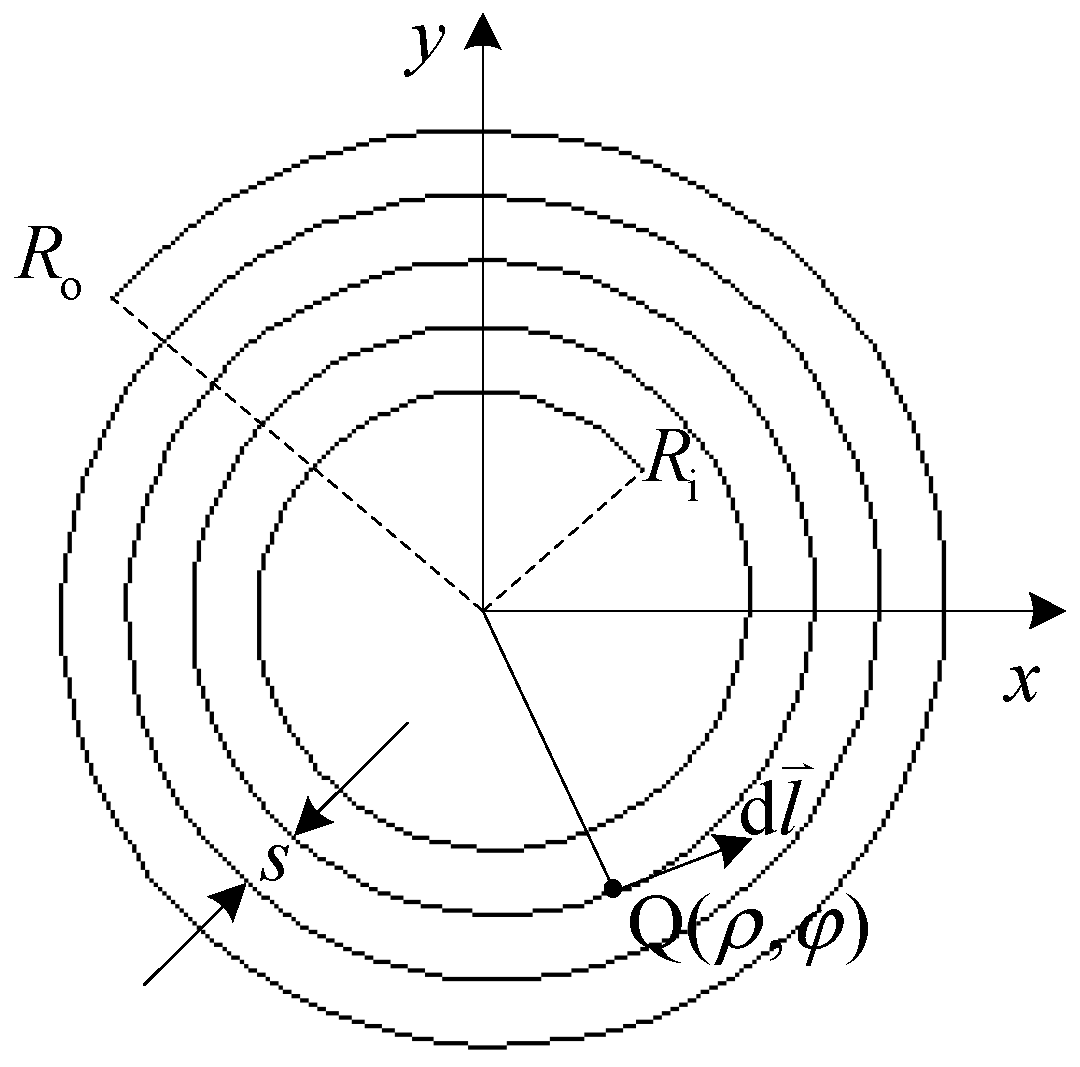
Figure 1 shows an Archimedean spiral curve, whose polar coordinate equation is [13]:

$$\rho =\frac{s}{2\pi }\phi ,{\mathsf{\Phi }}_{\mathrm{i}}\le \phi \le {\mathsf{\Phi }}_{\mathrm{o}},$$

(2)

where s is the screw pitch. Suppose R_i and R_o are the inner and outer radius of the spiral, respectively, and s/(2π) = a, so Φ_i = R_i/a; Φ_o = R_o/a.

Under the rectangular coordinate system, the equation of the spiral containing the parameter φ is:

$$\begin{array}{l}x=a\phi \cos \phi \\ y=a\phi \sin \phi \end{array}$$

(3)

Therefore, at a point Q on the spiral, the tangential vector is:

$$\begin{array}{l}\mathrm{d}\stackrel{\rightharpoonup }{l}=\mathrm{d}x\stackrel{\rightharpoonup }{\mathrm{i}}+\mathrm{d}y\stackrel{\rightharpoonup }{\mathrm{j}}=\\ a[(\cos \phi -\phi \sin \phi )\stackrel{\rightharpoonup }{\mathrm{i}}+(\sin \phi +\phi \cos \phi )\stackrel{\rightharpoonup }{\mathrm{j}}]\mathrm{d}\phi \end{array}$$

(4)

where i and j are unit vectors in the x and y direction, respectively.

A couple of coaxial Archimedean spiral coils C₁, C₂ are shown in Figure 2. The screw pitches of the spirals are s₁ and s₂, respectively, and the inner and outer radii are R_i1, R_o1, R_i2, and R_o2, respectively. The equations of C₁ and C₂ are as follows:

ρ₁ = a₁φ₁, Φ_i1 ≤ φ₁ ≤ Φ_o1, z₁ = 0;
ρ₂ = a₂φ₂, Φ_i2 ≤ φ₂ ≤ Φ_o2, z₂ = h;

where a₁ = s₁/(2π), a₂ = s₂/(2π), Φ_i1 = R_i1/a₁, Φ_o1 = R_o1/a₁, Φ_i2 = R_i2/a₂, and Φ_o2 = R_o2/a₂.

Q is taken arbitrarily from C₁, and P is taken arbitrarily from C₂. Expressing the rectangular coordinates with the cylindrical coordinates, the distance between the two points Q (ρ₁cosφ₁, ρ₁sinφ₁, 0) and P (ρ₂cosφ₂, ρ₂sinφ₂, h) is:

$$r={[{({\rho }_2\cos {\phi }_2-{\rho }_1\cos {\phi }_1)}^2+{({\rho }_2\sin {\phi }_2-{\rho }_1\sin {\phi }_1)}^2+h^2]}^{1/2}.$$

(5)

The tangential vector at points Q and P and their inner product are:

$$\mathrm{d}{\stackrel{\rightharpoonup }{l}}_1=a_1[(\cos {\phi }_1-{\phi }_1\sin {\phi }_1)\stackrel{\rightharpoonup }{\mathrm{i}}+(\sin {\phi }_1+{\phi }_1\cos {\phi }_1)\stackrel{\rightharpoonup }{\mathrm{j}}]\mathrm{d}{\phi }_1$$

$$\mathrm{d}{\stackrel{\rightharpoonup }{l}}_2=a_2[(\cos {\phi }_2-{\phi }_2\sin {\phi }_2)\stackrel{\rightharpoonup }{\mathrm{i}}+(\sin {\phi }_2+{\phi }_2\cos {\phi }_2)\stackrel{\rightharpoonup }{\mathrm{j}}]\mathrm{d}{\phi }_2$$

$$\mathrm{d}{\stackrel{\rightharpoonup }{l}}_1\cdot \mathrm{d}{\stackrel{\rightharpoonup }{l}}_2=a_1{a}_2[(1+{\phi }_1{\phi }_2)\cos ({\phi }_2-{\phi }_1)-({\phi }_2-{\phi }_1)\sin ({\phi }_2-{\phi }_1)]\mathrm{d}{\phi }_1\mathrm{d}{\phi }_2.$$

(6)

Substituting Equations (5) and (6) into Equation (1), the accurate expression of mutual inductance between coaxial Archimedean spiral coils can be obtained by:

$$M=\frac{{\mu }_0}{4\mathsf{\pi }}{a}_1{a}_2{\displaystyle {\int }_{{\mathsf{\Phi }}_{\mathrm{i}2}}^{{\mathsf{\Phi }}_{\mathrm{o}2}}{\displaystyle {\int }_{{\mathsf{\Phi }}_{\mathrm{i}1}}^{{\mathsf{\Phi }}_{\mathrm{o}1}}\frac{(1+{\phi }_1{\phi }_2)\cos ({\phi }_2-{\phi }_1)-({\phi }_2-{\phi }_1)\sin ({\phi }_2-{\phi }_1)}{\sqrt{h^2+a_1^2{\phi }_1^2+a_2^2{\phi }_2^2-2a_1{a}_2{\phi }_1{\phi }_2\cos ({\phi }_2-{\phi }_1)}}}}\mathrm{d}{\phi }_1\mathrm{d}{\phi }_2.$$

(7)

2.2. Numerical Calculation and Verification of the Accurate Expression of Mutual Inductance and Its Comparison with the Traditional Mutual Inductance Calculation Method

2.2.1. Method Proposed in This Paper

Equation (7) in this paper is a double integral, so its integrand can not be represented by an elementary function. Thus, the composite integral method combined with Gaussian quadrature formula with four points [20] is adopted to solve the double integrals numerically in the whole paper. As the integrand is a continuous function of the integral variables φ₁ and φ₂, the calculation precision of (7) can be increased through reducing the step length of the integral variables Δφ₁ and Δφ₂. The step length in this paper is set as π/16, to ensure that compared to the step size of π/32, the mutual inductance calculated in the following examples has the same first five or more significant digits. Thus, mutual inductance can be obtained for a couple of coaxial Archimedean spiral coils as shown in Figure 2 with known screw pitches, inner radii, and outer radii at different distances.

2.2.2. Conventional Circular Coils Approximation Method

In the traditional method, each planar spiral coil is approximate to a cluster of series-connected concentric circular coils. If the inner and outer radii of a spiral coil are R_i and R_o, respectively, there are N turns in the approximate cluster of concentric circular coils, so the radius of the innermost turn is R_i = R_o − (N − 1)s, and the radius of the jth turn is R_i + (j − 1)s, j = 1,2,…,N [14]. In this way, a couple of spiral coils as shown in Figure 2 is approximate to two clusters of concentric circular loops, and their number of turns are N₁ and N₂, respectively. The mutual inductance between such a couple of coils can be expressed as [2,14]:

$$M={\displaystyle \sum _{i=1}^{N_1}{\displaystyle \sum _{j=1}^{N_2}{M}_{ij}}}$$

(8)

where i and j represent the ith and jth turn of the two coils, respectively. M_ij is the mutual inductance between the ith approximate circular loop of C₁ (radius R_1i) and the jth approximate circular loop of C₂ (radius R_2j). M_ij is calculated by Maxwell’s formula [6]:

$$M_{ij}={\mu }_0\sqrt{R_{1i}{R}_{2j}}[(\frac{2}{m}-m)K(m)-\frac{2}{m}E(m)],$$

(9)

where $m=2\sqrt{\frac{R_{1i}{R}_{2j}}{h^2+{(R_{1i}+R_{2j})}^2}}$, K(m), and E(m) are complete elliptic integrals of the first and second kind [7]. The complete elliptic integral in (9) is approximated by the series expansion method.

2.2.3. Verification of the Method Proposed in This Paper and Its Comparison with the Traditional Methods

Equation (7) is an exact expression expressed by a double integral, which is concise in form and convenient to use. However, the traditional method is an approximation approach, which needs to calculate the radius of each circle of these two clusters of concentric coils, then through series expansion calculation and finally double summation, mutual inductance can be obtained.

The calculation results of Equation (7) are verified by the 3D finite element method (FEM). Their differences with the traditional method can be compared through the specific examples below, and the influences of coil parameters on mutual inductance can be studied. For a couple of coaxial spiral coils with five turns each, the solution type of the 3D FEM model is chosen as “Magnetostatic”, the current is uniformly distributed on the coil’s cross section, the mesh is assigned as “length based”, and the maximum length of elements is set as the default value.

(a) Variation of the distance

Table 1. Mutual inductance at different distances.

Distance h (m)	M3D (μH)	MS (μH)	ES (%)	MT (μH)	ET (%)
0.01	3.5665	3.6051	1.07	3.2244	10.6
0.03	2.1676	2.2125	2.03	1.9388	11.8
0.05	1.3932	1.4397	3.23	1.2373	12.6

shows the mutual inductance calculation results at three different distances for a couple of coaxial spiral coils with outer radii R_o1 = R_o2 = 0.1 m and screw pitches s₁ = s₂ = 0.01 m. M_3D stands for 3D FEM results; M_S represents the results of Equation (7) and E_S represents their errors relative to M_3D; M_T represents the results of the traditional circular coils approximation method and E_T represents their errors relative to M_3D.

(b) Variation of the screw pitches

Table 2. Mutual inductance at different screw pitches.

Screw Pitches s (m)	M3D (μH)	MS (μH)	ES (%)	MT (μH)	ET (%)
0.005	4.0277	4.0983	1.72	3.9093	3.03
0.010	2.7551	2.7974	1.51	2.4764	11.3
0.015	1.7232	1.7652	2.38	1.3824	24.7

shows the mutual inductance calculation results at three different screw pitches for a couple of coaxial spiral coils with R_o1 = R_o2 = 0.1 m and distances h = 0.02 m.

(c) Variation of the external radius

Table 3. Mutual inductance at different external radii.

External Radii Ro (m)	M3D (μH)	MS (μH)	ES (%)	MT (μH)	ET (%)
0.1	2.7551	2.7974	1.51	2.4764	11.3
0.2	10.776	10.912	1.25	10.452	3.10
0.3	20.625	20.984	1.71	20.453	0.843

shows mutual inductance calculation results at three different outer radii for a couple of coaxial spiral coils with h = 0.02 m and s₁ = s₂ = 0.01 m.

It can be seen from Table 1, Table 2 and Table 3 that:

(a) The calculation results of Equation (7) in this paper are close to that from Maxwell 3D with little difference. The test shows that the larger the 3D region of the simulation setting is, the smaller the differences are, but the simulation time will be longer.

(b) The relative errors between the traditional circular coils approximation method and the 3D FEM results are obvious. For the traditional method, the error increases with distances when outer radii and screw pitches are fixed; the error increases with screw pitches when outer radii and distances are fixed; the error decreases with outer radii when distances and screw pitches are fixed.

(c) The mutual inductance decreases with distances at fixed outer radii and screw pitches, decreases with screw pitches at fixed outer radii and distances, and increases with outer radii at fixed distances and screw pitches.

In terms of computational efficiency, for the above example, the calculation time of the proposed method is in the level of 10⁻¹ s, while the traditional method is in the level of 10⁻² s. However, it takes more than 10 h to simulate a 3D model established by ANSYS Maxwell considering the helicity.

3. Mutual Inductance between a Couple of Archimedean Spiral Coils with Lateral Misalignment

3.1. Accurate Expression of Mutual Inductance between Archimedean Spiral Coils with Lateral Misalignment

The relative position relationship of a couple of Archimedean spiral coils with lateral misalignment and with a distance h is shown in Figure 3.

C₁ is in the plane xoy and its axis passes through the origin; C₂ is in the plane z = h; d is the lateral misalignment, i.e., the distance between the axes of C₁ and C₂; O′′ is the projection of O′ on the xoy plane; and the angle between OO′′ and the x axis is α.

In this case, by adding the bases of the three terms in Equation (5) to the axial lateral shifting coordinate of C₂ (dcosα, dsinα, 0) and replacing the denominator of the integrand in Equation (7), exact expression of mutual inductance between Archimedean spiral coils C₁ and C₂ with lateral misalignment can be obtained by:

$$M=\frac{{\mu }_0}{4\mathsf{\pi }}{a}_1{a}_2{\displaystyle {\int }_{{\mathsf{\Phi }}_{\mathrm{i}2}}^{{\mathsf{\Phi }}_{\mathrm{o}2}}{\displaystyle {\int }_{{\mathsf{\Phi }}_{\mathrm{i}1}}^{{\mathsf{\Phi }}_{\mathrm{o}1}}\frac{(1+{\phi }_1{\phi }_2)\cos ({\phi }_2-{\phi }_1)-({\phi }_2-{\phi }_1)\sin ({\phi }_2-{\phi }_1)}{\sqrt{h^2+{(d\cos \alpha +a_2{\phi }_2\cos {\phi }_2-a_1{\phi }_1\cos {\phi }_1)}^2+{(d\sin \alpha +a_2{\phi }_2\sin {\phi }_2-a_1{\phi }_1\sin {\phi }_1)}^2}}}}\mathrm{d}{\phi }_1\mathrm{d}{\phi }_2.$$

(10)

If setting d = 0, Equation (10) will be simplified to Equation (7), i.e., Equation (7) is a special case of Equation (10).

3.2. The Influence of Distance and Lateral Misalignment on Mutual Inductance

The parameters of two parallel spiral coils C₁ and C₂ are given in

Table 4. Parameter of the spiral coils.

	Turns N	Screw Pitches s (mm)	Outer Radii Ro (mm)	Inner Radii Ri (mm)
C1	34	2.3529	105	25
C2	22	3.6364	105	25

. Equation (10) is solved numerically under different conditions.

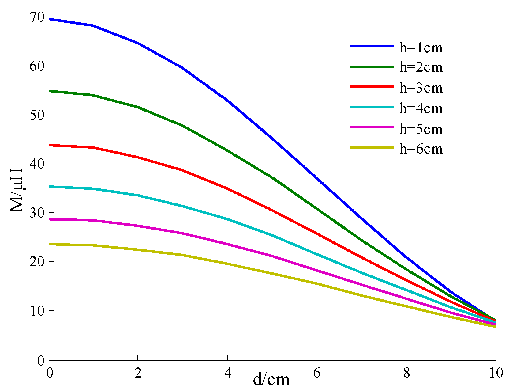
At a fixed distance h = 20 mm, the influence of lateral misalignment d and the azimuth angle α on mutual inductance M between the two spiral coils is shown in Figure 4.

It can be seen that M decreases obviously with d, while α has little influence on M.

At a fixed azimuth angle α = 0°, the influence of h and d on M is shown in Figure 5.

It can be seen that with the increase of h, M decreases, while the influence of d on M declines. Similarly, with the increase of d, M decreases, while the influence of h on M declines.

4. Mutual Inductance of Archimedean Spiral Coils with Arbitrary Relative Position

4.1. Mutual Inductance Expression of a Couple of Non-Parallel Archimedean Spiral Coils

The spatial position of a rigid body can be described by three translational degrees of freedom and three rotational degrees of freedom, and rotational degrees of freedom can be expressed by the Euler angle [21]. The Euler angle includes the precession angle, nutation angle, and spin angle. As can be seen from Figure 4, the precession angle and spin angle have little influence on the mutual inductance between spiral coils. Hence, only the case shown in Figure 6 needs to be studied: C₁ is in the plane xoy and its axis passes through the origin, O′(x₀,y₀,z₀) is the center of C₂, the axis of C₂ maintains parallel position to the plane xoz, and the nutation angle between its axis and the z axis is θ.

Under the rectangular coordinate system, the equation of C₁ containing the parameter φ₁ is:

x₁ = a₁φ₁cosφ₁, y₁ = a₁φ₁sinφ₁, z₁ = 0;

the equation of C₂ containing the parameter φ₂ is:

x₂ = x₀ + a₂φ₂cosφ₂cosθ, y₂ = y₀ + a₂φ₂sinφ₂, z₂ = z₀ − a₂φ₂cosφ₂sinθ,

thus:

$$\begin{array}{l}\mathrm{d}{\stackrel{\rightharpoonup }{l}}_1=a_1[(\cos {\phi }_1-{\phi }_1\sin {\phi }_1)\stackrel{\rightharpoonup }{\mathrm{i}}+(\sin {\phi }_1+{\phi }_1\cos {\phi }_1)\stackrel{\rightharpoonup }{\mathrm{j}}]\mathrm{d}{\phi }_1\\ \mathrm{d}{\stackrel{\rightharpoonup }{l}}_2=a_2[\cos \theta (\cos {\phi }_2-{\phi }_2\sin {\phi }_2)\stackrel{\rightharpoonup }{\mathrm{i}}+(\sin {\phi }_2+{\phi }_2\cos {\phi }_2)\stackrel{\rightharpoonup }{\mathrm{j}}-\sin \theta (\cos {\phi }_2-{\phi }_2\sin {\phi }_2)\stackrel{\rightharpoonup }{\mathrm{k}}]\mathrm{d}{\phi }_2\end{array}.$$

(11)

Combining Equation (1), the exact expression of mutual inductance in the case of Figure 6 can be obtained by:

$$M=\frac{{\mu }_0}{4\mathsf{\pi }}{a}_1{a}_2{\displaystyle {\int }_{{\mathsf{\Phi }}_{\mathrm{i}2}}^{{\mathsf{\Phi }}_{\mathrm{o}2}}{\displaystyle {\int }_{{\mathsf{\Phi }}_{\mathrm{i}1}}^{{\mathsf{\Phi }}_{\mathrm{o}1}}\frac{\cos \theta (\cos {\phi }_1-{\phi }_1\sin {\phi }_1)(\cos {\phi }_2-{\phi }_2\sin {\phi }_2)+(\sin {\phi }_1+{\phi }_1\cos {\phi }_1)(\sin {\phi }_2+{\phi }_2\cos {\phi }_2)}{\sqrt{{(x_0+a_2{\phi }_2\cos {\phi }_2\cos \theta -a_1{\phi }_1\cos {\phi }_1)}^2+{(y_0+a_2{\phi }_2\sin {\phi }_2-a_1{\phi }_1\sin {\phi }_1)}^2+{(z_0-a_2{\phi }_2\cos {\phi }_2\sin \theta )}^2}}\mathrm{d}{\phi }_1\mathrm{d}{\phi }_2}}$$

(12)

If θ = 0, and (x₀,y₀,z₀) in rectangular coordinates are expressed as (dcosα, dsinα, h) in cylindrical coordinates, Equation (12) will be simplified to Equation (10), i.e., Equations (7) and (10) are two special cases of Equation (12).

4.2. The Influence of Relative Rotational Angle on the Mutual Inductance of the Coils

The parameters of the two spiral coils C₁ and C₂ are given in Table 4. The values of x₀, y₀, z₀, and θ are selected properly to ensure that the two spiral coils do not cross. Equation (12) is solved numerically under different conditions.

Taking x₀ = y₀ = 0, the trend of M changing with θ at different values of z₀ is shown in Figure 7.

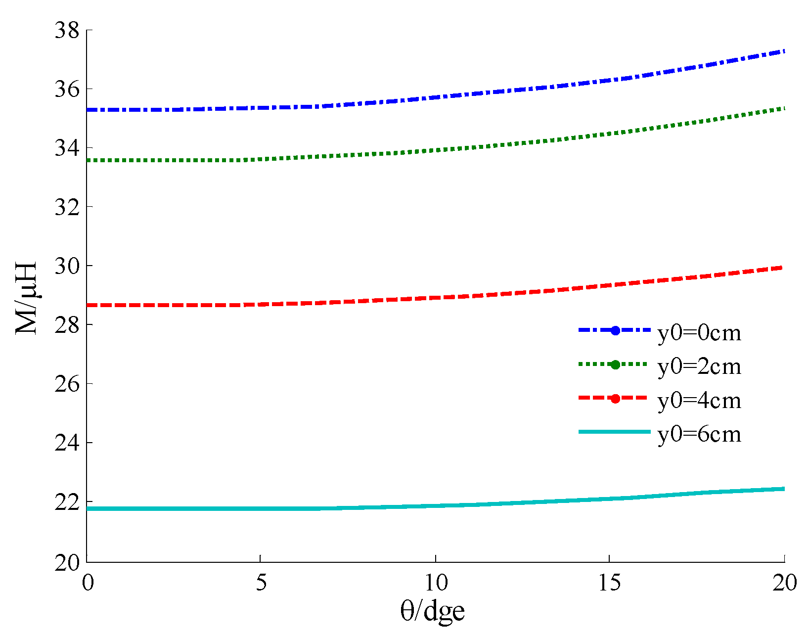
Taking x₀ = 0 and z₀ = 40 mm, the trend of M changing with θ at different values of y₀ is shown in Figure 8.

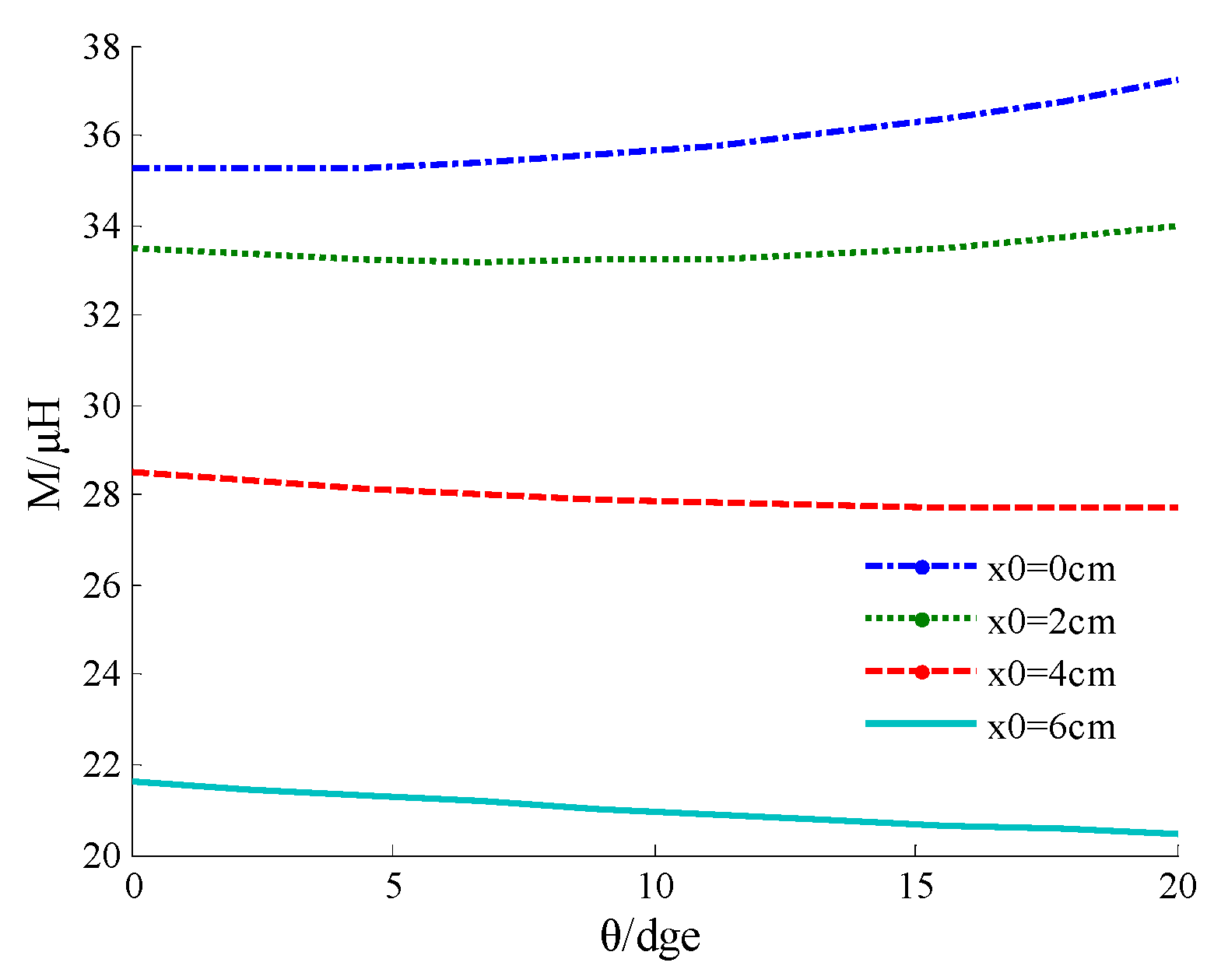
Taking y₀ = 0 and z₀ = 40 mm, the trend of M changing with θ at different values of x₀ is shown in Figure 9.

It can be seen that under smaller θ, in Figure 7, Figure 8 and Figure 9 with smaller x₀, M increases with θ, yet in Figure 9 with larger x₀, M decreases with θ.

5. Interpretation of the Relationship between Mutual Inductance and Relative Position of Archimedean Spiral Coils from the Perspective of Magnetic Field Distribution

In order to further explain the relationship between the relative position of a couple of Archimedean spiral coils and their mutual inductance, it is necessary to analyze the magnetic field spatial distribution of a single current-carrying Archimedean spiral coil. Let us assume that a spiral coil C₁ carrying current I is located in the plane xoy and its axis is the z axis. The coordinate of the detecting point P is (x,y,z). According to the Biot–Savart law, the magnetic induction intensity at point P can be expressed as:

$$\stackrel{\rightharpoonup }{B}=\frac{{\mu }_{0}I}{4\mathsf{\pi }}{\displaystyle \int \frac{\mathrm{d}\stackrel{\rightharpoonup }{l}\times \stackrel{\rightharpoonup }{r}}{r^3}},$$

(13)

where:

$$\begin{array}{l}\stackrel{\rightharpoonup }{r}=(x-a\phi \cos \phi )\stackrel{\rightharpoonup }{\mathrm{i}}+(y-a\phi \sin \phi )\stackrel{\rightharpoonup }{\mathrm{j}}+z\stackrel{\rightharpoonup }{\mathrm{k}}\\ r^2={(x-a\phi \cos \phi )}^2+{(y-a\phi \sin \phi )}^2+z^2\\ \mathrm{d}\stackrel{\rightharpoonup }{l}=a[(\cos \phi -\phi \sin \phi )\stackrel{\rightharpoonup }{\mathrm{i}}+(\sin \phi +\phi \cos \phi )\stackrel{\rightharpoonup }{\mathrm{j}}]\mathrm{d}\phi \end{array}.$$

Each component of $\stackrel{\rightharpoonup }{B}$ can be expressed as:

$$B_x=\frac{{\mu }_{0}I}{4\mathsf{\pi }}az{\displaystyle {\int }_{{\mathsf{\Phi }}_{\mathrm{i}}}^{{\mathsf{\Phi }}_{\mathrm{o}}}\frac{(\sin \phi +\phi \cos \phi )}{r^3}\mathrm{d}\phi }$$

(14)

$$B_y=\frac{{\mu }_{0}I}{4\mathsf{\pi }}az{\displaystyle {\int }_{{\mathsf{\Phi }}_{\mathrm{i}}}^{{\mathsf{\Phi }}_{\mathrm{o}}}\frac{(\phi \sin \phi -\cos \phi )}{r^3}\mathrm{d}\phi }$$

(15)

$$B_z=\frac{{\mu }_{0}I}{4\mathsf{\pi }}a{\displaystyle {\int }_{{\mathsf{\Phi }}_{\mathrm{i}}}^{{\mathsf{\Phi }}_{\mathrm{o}}}\frac{(y-x\phi )\cos \phi -(x+y\phi )\sin \phi +a{\phi }^2}{r^3}\mathrm{d}\phi }$$

(16)

It can be seen from Equations (14)–(16) that B_x(–z) = –B_x(z), B_y(–z) = –B_y(z), B_z(–z) = B_z(z), and B_x = B_y = 0 on the plane xoy where the spiral coil is located. This indicates that the magnetic field distribution has symmetry with respect to the plane xoy.

The parameters of C₁ are given in Table 4, which carries the current of 6A. The contour map of B_z on the plane y = 0 is drawn according to the numerical calculation of Equation (16), as shown in Figure 10.

The contour map of B_z on the plane z = 2 cm is drawn as shown in Figure 11.

The influence of relative position on the mutual inductance of a couple of parallel Archimedean spiral coils in Figure 4 and Figure 5 can be explained by Figure 10 and Figure 11. The farther away the two coils are, the weaker the magnetic field is, and thus the smaller the mutual inductance will be. The distribution of B_z in Figure 11 is almost axial symmetric, hence α has little influence on M in Figure 4.

The distribution of the tangential magnetic field $B_x\stackrel{\rightharpoonup }{\mathrm{i}}+B_z\stackrel{\rightharpoonup }{\mathrm{k}}$ module (contour map) and direction (arrow) on the plane y = 0 is shown in Figure 12.

Supposing that above the coil C₁, there is another coil C₂ with a fixed center O′ and tilted axis as shown in Figure 6, when the axis of C₂ is parallel to the plane xoz and its tilt angle θ is small, Figure 7, Figure 8 and Figure 9 can be explained as follows:

When O′ is on the z axis (as shown in Figure 7) or directly above the y axis (as shown in Figure 8), it can be seen by combining Figure 6 with Figure 12 that the magnetic flux of the lower part of C₂ increases with θ due to the normal magnetic field increases, yet the flux of the upper part decreases with θ. As the lower part of C₂ is closer to C₁, it has a greater contribution to the flux than the upper part, i.e., the mutual inductance between C₁ and C₂ increases with θ.

For the case that O′ is directly above the x axis as shown in Figure 9, while x₀ is smaller, similar to the case in Figure 7 when O′ is on the z axis, M increases with θ; however, while x₀ is larger, as the upper part of C₂ is closer to C₁, its contribution to the flux is greater than the lower part, and M decreases with θ.

6. Experimental Verification

In order to verify the correctness of the mutual inductance calculation method proposed in this paper, a couple of Archimedean spiral coils C₁ and C₂ (their parameters are shown in Table 4) were fabricated with Litz wire (the diameter of each strand of wire was 0.1 mm, so the skin effect could be ignored under the testing frequency of 100 kHz), as shown in Figure 13.

These two spiral coils were fixed on the square insulating hardboard, and the lateral misalignment d, i.e., the distance between the axes of the two parallel coils could be adjusted conveniently by the scales on the insulating board. The distance h between two parallel coils could also be conveniently adjusted by placing a hard insulating block of known thickness between the two insulating hardboards (considering the thickness of the coils, h started from the horizontal cross-section of each coil). The method for measuring mutual inductance was as follows: First measure the inductance values when the two coils are in the same directional series and in reverse directional series, respectively, then subtract the two values and divide them by 4 [22]. The measuring instrument was a type 3250 transformer tester produced by Chroma, and the testing frequency was selected as 100 kHz.

First, the mutual inductance of the two spiral coils in Figure 13 was measured in parallel state, under conditions of different d and h, and compared with the mutual inductance calculated by Equation (10), the results were sorted out as shown in Figure 14.

The calculation results in Figure 14 are equivalent to that in Figure 7 (observing some special points with the same h and d). As can be seen from Figure 14, similar to the simulation results in Table 1, the relative error between the measurement result and the calculation result increased with h.

Then, a wedge with a 20° angle of gradient was machined using easy cutting insulation materials such as hard foam, C₁ and θ = 20° were fixed according to Figure 6, and x₀, y₀, z₀ were adjusted.

Taking x₀ = y₀ = 0, the mutual inductance measurement results and calculation results according to Equation (12) at different values of z₀ are listed in

Table 5. Mutual inductance when θ = 20° and x₀ = y₀ = 0.

z0 (mm)	M (μH) Measured	M (μH) Calculated	Relative Error (%)
40	37.33	37.35	0.05
50	30.50	30.08	1.40
60	23.84	24.46	2.53

.

The calculation results in Table 5 are three special points taken from Figure 7.

Taking y₀ = 0, z₀ = 40 mm, the mutual inductance measurement results and calculation results according to Equation (12) at different values of x₀ are listed in

Table 6. Mutual inductance when θ = 20°, y₀ = 0, and z₀ = 40 mm.

x0 (mm)	M (μH) Measured	M (μH) Calculated	Relative Error (%)
20	34.02	34.08	0.18
40	27.70	27.80	0.36
60	20.32	20.54	1.07

.

The calculation results in Table 6 are three special points taken from Figure 9.

Taking x₀ = 0, z₀ = 40 mm, the mutual inductance measurement results and calculation results according to Equation (12) at different values of y₀ are listed in

Table 7. Mutual inductance when θ = 20°, x₀ = 0, and z₀ = 40 mm.

y0 (mm)	M (μH) Measured	M (μH) Calculated	Relative Error (%)
20	35.23	35.45	0.64
40	30.16	30.06	0.33
60	22.45	22.59	0.62

.

The calculation results in Table 7 are three special points taken from Figure 8.

As can be seen from Figure 14 and Table 5, Table 6 and Table 7, the calculation results by the accurate expressions were in good agreement with the experimental results. Their relative error was within 3 %, and it increases obviously with h, d and z₀.

7. Conclusions

Aiming at improving the calculation accuracy of the mutual inductance of Archimedean spiral coils, this paper proposed accurate expressions of mutual inductance that considered the helicity of the coils and corresponding numerical calculation methods. The expressions of mutual inductance when the two coils are in different relative positions were given in the form of a double integral, and Gaussian integral method was used to solve these expressions numerically. For the coaxial case, 3D FEM results were taken as reference values, and the proposed method was compared with the traditional method. The simulation results showed that the traditional method without considering the helicity of the coils had a larger error, especially when the pitches were wider. The influence of the relative position of the two coils on mutual inductance was also studied and explained by magnetic field distribution. Finally, a couple of Archimedean spiral coils were fabricated to verify the theoretical formula. The experimental results showed that the relative error of the mutual inductance calculation method proposed in this paper was within 3 %, which confirms the correctness of the theoretical formula.

References

- Nguyen, M.Q.; Hughes, Z.; Woods, P.; Seo, Y.S.; Rao, S.; Chiao, J.C. Field Distribution Models of Spiral Coil for Misalignment Analysis in Wireless Power Transfer Systems. IEEE Trans. Microw. Theory Tech. 2014, 62, 920–930. [Google Scholar] [CrossRef]
- Raju, S.; Wu, R.; Chan, M.; Yue, C.P. Modeling of Mutual Coupling Between Planar Inductors in Wireless Power Applications. IEEE Trans. Power Electron. 2014, 29, 481–490. [Google Scholar] [CrossRef]
- Hurley, W.G.; Duffy, M.C. Calculation of Self and Mutual Impedances in Planar Magnetic structures. IEEE Trans. Magn. 1995, 31, 2416–2422. [Google Scholar] [CrossRef]
- Rana, M.; Xiang, W. IoT Communications Network for Wireless Power Transfer System State Estimation and Stabilization. IEEE Internet Things J. 2018, 5, 4142–4150. [Google Scholar] [CrossRef]
- Rana, M.; Xiang, W.; Wang, E.; Li, X.; Choi, B.J. Internet of Things Infrastructure for Wireless Power Transfer Systems. IEEE Access 2018, 6, 19295–19303. [Google Scholar] [CrossRef]
- Maxwell, J.C. A Treatise on Electricity and Magnetism; Oxford Clarendon Press: Oxford, UK, 1873. [Google Scholar]
- Good, R.H. Elliptic integrals, the forgotten functions. Eur. J. Phys. 2001, 22, 119–126. [Google Scholar] [CrossRef]
- Kalantarov, P.L. Inductance Calculations; National Power Press: Moscow, Russia, 1955. [Google Scholar]
- Ramo, S.; Whinnery, J.R.; Duzer, T.V. Fields and Waves in Communication Electronics; John Wiley & Sons Inc.: Hoboken, NJ, USA, 1994. [Google Scholar]
- Havelock, T.H. On Certain Bessel Integrals and the Coefficients of Mutual Induction of Coaxial Coils. Lond. Edinb. Dublin Philos. Mag. J. Sci. 1908, 15, 332–345. [Google Scholar] [CrossRef]
- Babic, S.I.; Sirois, F.; Akyel, C. Validity Check of Mutual Inductance Formulas for Circular Filaments with Lateral and Angular Misalignments. Prog. Electromagn. Res. 2009, 8, 15–26. [Google Scholar] [CrossRef]
- Babic, S.; Sirois, F.; Akyel, C.; Girardi, C. Mutual Inductance Calculation Between Circular Filaments Arbitrarily Positioned in Space: Alternative to Grover’s Formula. IEEE Trans. Magn. 2010, 46, 3591–3600. [Google Scholar] [CrossRef]
- Lockwood, E.H. A Book of Curves; Cambridge University Press: Cambridge, MA, USA, 2007. [Google Scholar]
- Khan, S.R.; Pavuluri, S.K.; Desmulliez, M.P.Y. Accurate Modeling of Coil Inductance for Near-Field Wireless Power Transfer. IEEE Trans. Microw. Theory Tech. 2018, 66, 4158–4169. [Google Scholar] [CrossRef]
- Luo, Z.; Wei, X. Analysis of Square and Circular Planar Spiral Coils in Wireless Power Transfer System for Electric Vehicles. IEEE Trans. Ind. Electron. 2018, 65, 331–341. [Google Scholar] [CrossRef]
- Raju, S.; Wu, R.; Chan, M. Modeling of Mutual Inductance for Planar Inductors Used in Inductive Link Applications. In Proceedings of the 2012 IEEE International Conference on Electron Devices and Solid State Circuit (EDSSC 2012), Bangkok, Thailand, 3–5 December 2012; pp. 1–2. [Google Scholar]
- Zierhofer, C.M.; Hochmair, E.S. Geometric approach for coupling enhancement of magnetically coupled coils. IEEE Trans. Biomed. Eng. 1996, 43, 708–714. [Google Scholar] [CrossRef] [PubMed]
- Covic, G.A.; Boys, J.T. Modern Trends in Inductive Power Transfer for Transportation Applications. IEEE J. Emerg. Sel. Top. Power Electron. 2013, 1, 28–41. [Google Scholar] [CrossRef]
- Zhou, X.; Chen, B.; Luo, Y.; Zhu, R. Analytical Calculation of Mutual Inductance of Finite-Length Coaxial Helical Filaments and Tape Coils. Energies 2019, 12, 566. [Google Scholar] [CrossRef]
- Jacques, I.; Judd, C. Numerical Analysis; Chapman and Hall: London, UK, 2011. [Google Scholar]
- Mondal, C.R. Classical Mechanics; Phi Learning Pvt Ltd.: New Delhi, India, 2008. [Google Scholar]
- Su, Y.P.; Liu, X.; Ronhui, S.Y. Mutual Inductance Calculation of Movable Planar Coils on Parallel Surfaces. IEEE Trans. Power Electron. 2009, 24, 1115–1124. [Google Scholar] [CrossRef]
Figure 1.
An Archimedean spiral curve.
Figure 2.
Coaxial Archimedean spiral coils.
Figure 3.
Archimedean spiral coils with lateral misalignment.
Figure 4.
Influence of horizontal relative position on mutual inductance.
Figure 5.
Influence of distance and lateral misalignment on mutual inductance.
Figure 6.
A couple of non-parallel Archimedean spiral coils.
Figure 7.
Relationship between M and θ under different values of z0.
Figure 8.
Relationship between M and θ under different values of y0.
Figure 9.
Relationship between M and θ under different values of x0.
Figure 10.
Bz distribution on the y = 0 plane.
Figure 11.
Bz distribution on the z = 2 plane.
Figure 12.
Module and direction distribution of the tangential magnetic field on the y = 0 plane.
Figure 13.
Archimedean spiral coils sample.
Figure 14.
Comparison of mutual inductance measurement results and calculation results of a couple of spiral coils with lateral misalignment.