Experimental and Numerical Investigation of Bubble–Bubble Interactions during the Process of Free Ascension

Fundamental Science on Nuclear Safety and Simulation Technology Laboratory, Harbin Engineering University, Harbin 150001, China
*
Author to whom correspondence should be addressed.
Energies 2019, 12(10), 1977; https://doi.org/10.3390/en12101977
Submission received: 10 March 2019
/
Revised: 13 May 2019
/
Accepted: 14 May 2019
/
Published: 23 May 2019
Abstract
:The shape and rising behavior of the horizontally arranged twin bubbles in a steady liquid are experimentally studied employing high-speed photography and digital image processing, and numerically studied by the Volume-Of-Fluid (VOF) method, in combination with a momentum equation coupled with a surface tension model. The movement trajectory and the velocity variation in horizontal and vertical directions of the horizontally arranged twin bubbles rising side by side, as observed in experiments, are described. According to the results, when two bubbles rise side by side, their horizontal velocity changes by the simple harmonic law; there is a cyclical process of two bubbles repeatedly attracted to and bounced against each other, rather than at constant distance between each other, and the bubbles swing up and down periodically in the water. The mathematical model and its numerical implementation are presented in detail. The validation of the model is confirmed by comparing the numerical and experimental results, which are in good agreement with each other; the numerical simulation can accurately reproduce the deformation, attraction, and repulsion of the bubble pairs. The phenomenon of attraction and repulsion is comprehensively analyzed from the viewpoint of a flow field. It is considered that the interaction between the bubbles is mainly influenced by the changes of the flow field due to vortex counteraction and wake merging effects.
1. Introduction
The gas–liquid two-phase flow phenomenon exists widely in the chemical, petroleum, nuclear power, and new energy industries, such as solar energy and biogas energy, and many other fields [1,2,3,4]. It is important to gain a more fundamental understanding of the interaction mechanism between the bubble and its surrounding flow field in two-phase flow. Bubble dynamics has been recognized as an important topic, and many investigators focus on the study of bubble dynamics [5,6,7,8,9]. Wittke and Chao [10] studied the collapse of a spherical bubble when it was in transitory motion. Choi et al. [11] studied single bubble behavior characteristics and the flow field distribution in gas–liquid two-phase flow. Zhu et al. [12] discussed bubble formation, motion, and the evolution of the bubbling features, including bubble size, shape, and velocity.
In actual industrial processes, a lot of bubbles with different shapes, sizes, and velocity influence each other in equipment. The engineering application effect lies largely on the bubble behavior characteristics and the interaction between the continuous phase and dispersed phase [13,14]. Furthermore, the motion of multiple bubbles is different from that of single bubbles because of the complexity of their motion characteristics. Therefore, research on bubble movement characteristics and their interaction are of great value and academic significance for many engineering fields [15,16,17,18].
According to the experimental study on the interaction between two continuous bubbles in a vertical pipe, Talvy et al. [19] believed that the movement characteristics of the two bubbles were mainly determined by the forward bubble. Rzehak et al. [20] carried out theoretical analysis of the forces acting on two bubbles with different positions, proposing a new model of bubble coalescence and fragmentation. Karapantsios et al. [21] conducted experimental research on the collision process of two bubbles and established a theoretical model of the velocity and trajectory of a small bubble when it approaches a large bubble. Rodrigo [22] studied the interaction of two bubbles rising in shear-thinning inelastic fluids. Hallez and Legendre [23] studied the interaction between two bubbles for medium Reynolds numbers, and obtained a simple model based on physical parameters for the drag and lift of each bubble.
At present, the main testing methods are probe technology and high-speed photography technology. As the probe techniques [24] require direct contact with the gas phase to measure bubble size and gas hold-up in the system, the measurement of bubble behavior characteristics based on high-speed photography has become increasingly important due to its merits of non-contact, instantaneous, and full-field measurement [25].
Based on visual experimental studies of the generation characteristics of underwater single-porosity bubbles, Muller et al. [26] found that the bubble size increased with the increase of gas velocity in the case of large gas velocity. Monica et al [27] designed a photogrammetric 3D-PTV system to lengthen the trajectories and improve the statistical accuracy. Xue et al. [28] established a virtual binocular stereo vision system based on dual perspective imaging and studied the behavior characteristics of bubbles in gas–liquid two-phase flow. Belden et al. [29] developed an imaging system comprised of nine high-speed cameras, to record the bubbly flows induced by a turbulent circular plunging jet. Stewart [30], using a video camera, conducted experimental research on freely rising ellipsoidal bubbles approaching each other. Brucker [31] used digital particle image velocimetry and high-speed recording technology to study the wake flow of a single bubble and two interacting bubbles rising freely in water and found that the wake dynamics strongly triggered the bubble interaction by releasing two bubbles at the same time.
Although the phenomenon of bubble motion alongside growth can be explained qualitatively as demonstrated in some experimental investigations, the main difficulty in quantitative prediction is that the studies of multiphase flows present very complicated problems [32]. With the advancements in numerical technique and computing power over the last few decades, computational fluid dynamics (CFD) has become a very effective means of studying bubble behavior [33,34,35,36]. Yong Li et al. [37,38,39,40] simulated the deformation of a single bubble rising under high pressure using the volume-of-fluid (VOF) method. Furthermore, Hua et al. [41] presented a robust algorithm for direct numerical simulation of three-dimensional incompressible two-phase flow. The method described was applied to simulate three-dimensional bubbles rising in viscous liquids, and the interaction between two bubbles in liquids was simulated using the model. Chen et al. [42] simulated the rise of a single bubble in still water and its interaction with the gas–water interface by means of the VOF method.
Under actual working condition, bubbles often exist in the form of bubble groups, and bubble–bubble interactions have a unique effect on bubble behavior. Therefore, the research on the laws of the interaction between bubbles and mutual influences is quite significant. Previous studies on double bubbles have almost focused on bubble coalescence, less research has been done on the phenomenon of bubbles rising side by side, especially the effect of double inlet-orifice characteristics on bubbling performance. In this paper, visual experiments were conducted to study the influence of orifice spacing and orifice diameter on the bubbling performance. We also wanted to study the motion characters of two bubbles rising side by side, so we employed numerical simulation to analyze bubbles’ trajectories and the time dependencies of the relative location of the bubbles and of the flow velocity around them to explain the behavior observed in the experiments, which was not yet done in the literature. Then, we compared the results of numerical and experimental studies; the comparison shows good agreement between them.
2. Mathematical Model
2.1. Geometric Model
In this paper, the two bubbles rising side by side were numerically simulated. The simulated working condition was a rectangular channel (the working medium was water) of 40 mm × 100 mm. Two spherical bubbles with diameters of 5 mm were horizontally distributed side by side from the bottom of the container at 5 mm, and the initial horizontal distance between the two bubbles was 8 mm. The boundary conditions of inlet and outlet are velocity inlet and outflow. In this paper, the static water condition is simulated, so the inlet velocity is set to 0. The dimensionless Morton number (Mo) is defined by Equation (1). Physical parameters of liquid and gas in the simulation are listed in Table 1 [43].
where g, are water density, air density, water viscosity, gravity acceleration, surface tension coefficient, respectively.
The effect of mesh size on simulation results was tested by simulating the rise of a single bubble with a diameter of 5 mm in stationary water. The grid resolutions tested were 0.05 mm, 0.1 mm, 0.2 mm, and 0.4 mm, respectively. The simulation results of bubble rising velocity with different mesh sizes are shown in Figure 1. It can be seen from the figure that the final stabilization velocity of bubbles was approximately the same with mesh sizes of 0.05 mm and 0.1 mm. Considering the accuracy and computing time, the mesh size of 0.1 mm and grid number of 4 × 10⁵ were adopted in this study.
2.2. Governing Equations and Models
2.2.1. Gas Volume Fraction Equation
The liquid volume fraction equation has the same form as the gas volume fraction equation, and they satisfy the following condition:
where , t, x, y are water density, air density, water viscosity, air viscosity, water volume fraction, air volume fraction, time, Cartesian coordinates in x-axis and y-axis, respectively.
2.2.2. Momentum Conservation Equation
In Equation (4), F represents the surface tension force per unit volume which is considered by applying the continuum surface force model proposed by Brackbill et al. [44].
2.2.3. Surface Tension Model
The surface tension model in ANSYS Fluent software is the continuum surface force model. Consider the effect of surface tension on a fluid interface. The surface stress boundary condition at an interface between water and air (labeled l and g) is
where and is the pressure in water and air, respectively, is the fluid surface tension coefficient (in units of force per unit length), is the viscous stress tensor, is the unit normal (into air phase) at the interface, and is the local surface curvature.
In this paper, assuming that the surface tension coefficient is constant, each phase of the fluid is incompressible, and the effect of the viscosity at the interface is neglected. Based on this condition, Equation (6) can be simplified to Equation (7). Under the action of surface tension, the interfacial pressure difference between two-phase fluids is:
Surface pressure is therefore proportional to the curvature () of the interface. The higher pressure is in the fluid medium on the concave side of the interface, since surface tension results in a net normal force directed toward the center of the curvature of the interface.
In its standard form, surface tension contributes a surface pressure (Equation (7)) that is the normal force per unit interfacial area A at points xs on A, , where is the normal force component of the total surface force, Here, we consider interfaces between inviscid fluids having a constant surface tension coefficient, where . The surface force per unit interfacial area then can be written as
Consider a volume force, FSV (x), which gives the correct surface tension force per unit interfacial area, FSV (x), as h → 0:
where h is the thickness of the gas-liquid interface, its length comparable to the resolution afforded by a computational mesh with spacing ∆x.
Using Gauss’ theorem and Laplace transform method and noting that is constant within each fluid, one can convert the volume integral to an integral over the interface A; we find that
As h → 0, the corresponding limit of the integral of across the interface is given by
where is the jump in , . Thus, the limit h → 0 of can be written
This delta function can be used to rewrite FSA (x) as a volume integral for h = 0:
Upon substituting Equation (11) into Equation (12), we found that
By comparing Equation (9) with Equation (13), we identify the volume force, as
One can multiply the integrand on the right side of Equation (14) by the function without changing the value of the integral in the limit , since at the interface, x = xs and j(xs) = 1. If, for incompressible flow, j(x) is given by Equation (15) [44].
where , and the volume force in Equation (14), when multiplied by j(x), becomes
In the transition region, where the varies smoothly from to , the volume force is designed to simulate the surface pressure on the interface between the fluids. Thus, the line integral of across the transition region:
where ; with this model, the addition of surface tension to the VOF calculation results in a source term in the momentum equation (Equation (4)); the in Equation (4), has the following form:
The properties appearing in the transport equations are determined by the presence of the component phases in each control volume:
2.3. Interaction of Bubbles Model Description
Kok proposed the theoretical model of double bubble motion [45,46]. Vries simplified the model to study the interaction between bubbles and a wall surface [47]. Furthermore, Sanada believed that the simplified model was still applicable to the study of double bubble motion [48]. Therefore, the simplified model is used in this paper to analyze the movement of side-by-side bubbles,
In Equations (21) and (22), x denotes the distance between the two bubbles’ centers and the axis of the two bubbles; y is the height of the bubble’s center of mass; VB is the volume of the bubble; Mx and My are accessory mass coefficients; and Fx and Fy are external force terms. In the Kok model, external force terms are generated by buoyancy and viscosity. Dx and Dy are the drag forces.
where is the equivalent radius of the spherical bubble.
According to the Kok model, bubbles are always spherical. However, bubbles will be deformed in the rising process, and the lift force generated by bubble deformation will affect the movement of bubbles. Therefore, lift force needs to be added into the model. In the Vries model, the external force term is expressed as follows, where 2Lcosβ is the lift force generated by bubble deformation.
where is the angle made by the path with the horizontal.
3. Experimental Apparatus and Procedure
3.1. Experimental Apparatus
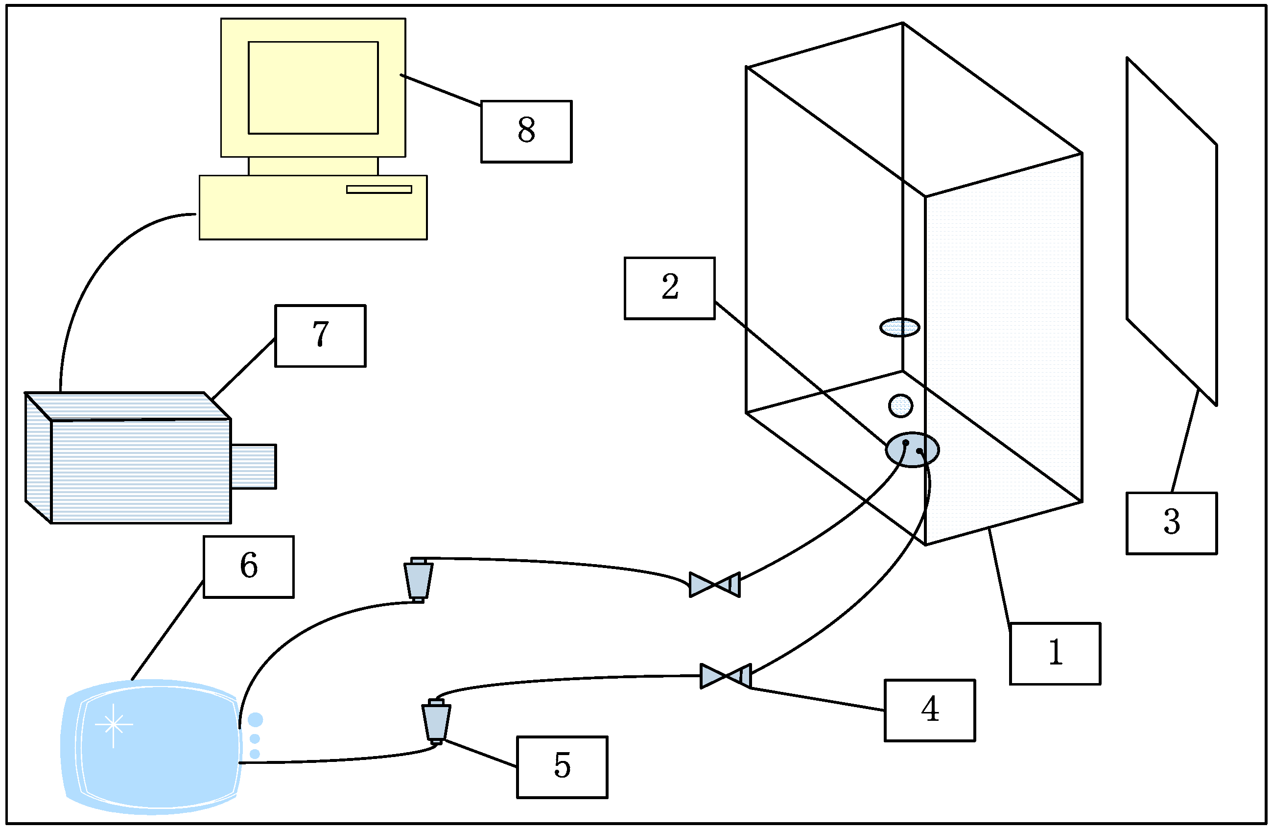
Figure 2 is a schematic diagram of the experimental system. The experimental device is composed of a water tank, bracket, float flow meter, LED plane light source, bubble generation module, check valve, air pump, high-speed camera, and computer. The visual water tank was a transparent container, which was made of organic glass. Its size was 300 mm × 300 mm × 300 mm, and the shoot direction size was 300 mm × 500 mm. It contained pure water with the height of 300 mm; inside orifices at the bottom of the tank were used to install the bubble generation component. Two orifices of the same diameter were drilled into the bubble generation component, as seen in Figure 3. The aperture outer diameter was 2 mm, and the distance, d, between two holes was 8 mm. The gas was provided by an electromagnetic vibrating air flow pump; in the experiment, a tiny flow glass rotor flow meter with a range of 16–160 mL/min was selected to control the gas flow into the gas orifice by adjusting the float flow meter. The formation process of bubbles was captured by a high-speed camera instrument.
3.2. Image Processing and Parameter Measurement
3.2.1. Image Processing Method
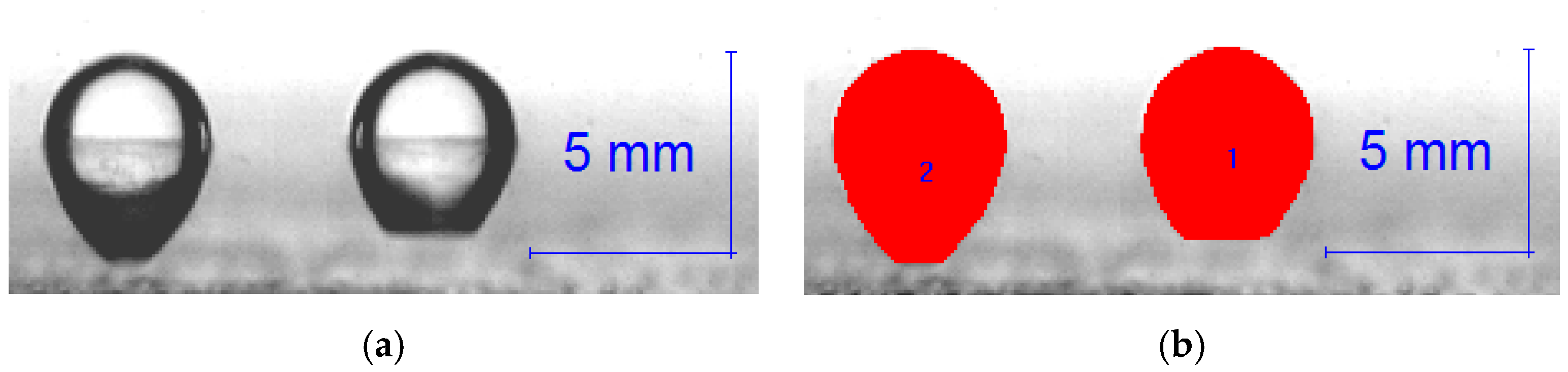
In the experiment, IPP (Image-Pro Plus) software was used to process the video shots frame by frame. Bubbles were approximately spherical when they escaped but showed irregular shapes in the subsequent movement process. Image edge area could be automatically identified and separated through IPP software. AOI (Area of Interest) was selected for measurement. In the case of very serious background interference, AOI could also be manually selected for measurement, with the measurement parameters including coordinates, distance, and area. As shown in Figure 4, the ruler and the fitting boundary of bubbles were obtained by using IPP.
3.2.2. Calculation of Bubble Parameters
The size, velocity, and position of bubbles are key feature parameters in the transport process. During the experiment, the shooting speed of the high-speed camera was certain, and the time difference of each frame image was known. Therefore, the characteristic parameters of the bubbles could be obtained by comparing the position and size differences of bubbles in the two frames of images, and then the rising trajectories, detachment size, and velocity change regulation could be tracked.
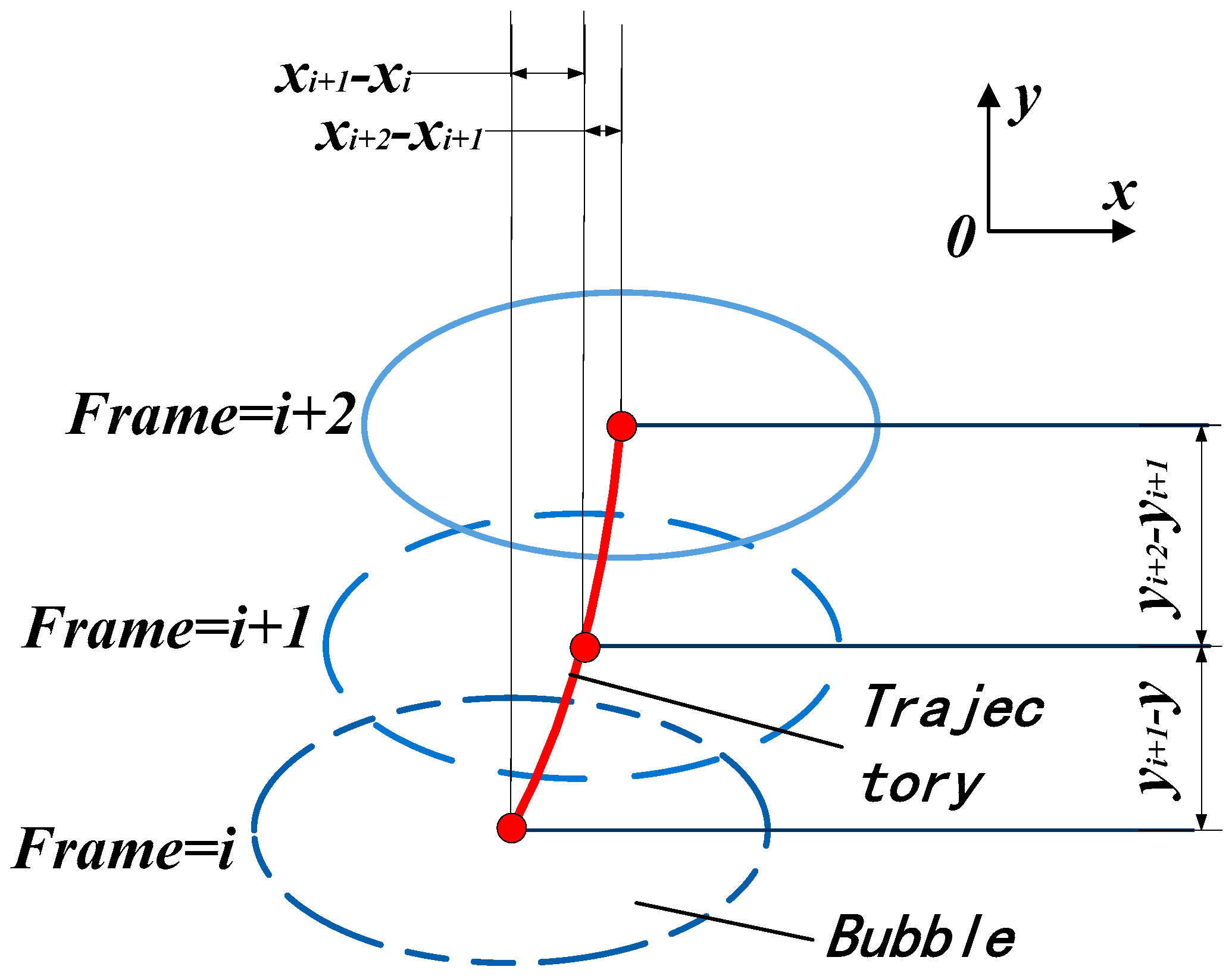
The profiles of a bubble in three adjacent images are shown in Figure 5. Its velocity was calculated in term of its centroid positions at two adjacent frames and the time interval:
where and are the velocity component in x and y directions, respectively, and δt is the time interval with a fixed value of 1 ms in current experiments.
3.2.3. Uncertainty Analysis
The measurement accuracies of bubble parameters are crucial for the reliability of the subsequent analysis. When flow rate of gas is directly measured, uncertainties are usually determined by the characteristics of measurement instruments themselves. The uncertainty of flow measurement is 2.5% without considering the accuracy of operation and reading error.
Besides, for experimental measurement errors, image resolution also induces uncertainties during detection of the bubble edge by digital image analysis in the measurements of bubble size and motion parameters, the uncertainties of these parameters are determined by using the error transfer principle, and calculated by Equation (34)
where N is an indirect measurement parameter, A, B, C are direct measurement parameters,
In the experiment, the filming frame rate was set to 5000 fps, that is, the shooting time interval is t = 0.2 ms, and the shutter time is ∆t = 1us, Save 1 picture every 10 frames, The time interval between the two saved pictures is ∆T = 10t, so the uncertainty of time is
Into the data, it can be obtained
In the experiment, the filming resolution is 1240 × 1240 pixels, the corresponding physical scale of the view window was about 100 × 180 mm2. Since the uncertainty for locating the position was within ±0.5 pixels, the maximum error of bubble location in the x direction was limited to ±0.049 mm, and the maximum error of bubble location in the y direction was limited to ±0.09 mm. The maximum error of bubble diameter was limited to ±0.09 × 2 = ±0.18 mm. In the experiment, the diameter of the bubbles was more than 4.3 mm. The uncertainty of bubble diameter was: 0.18 ÷ 4.3 × 100% = 4.18%.
Bubble velocity error is affected by both bubble size error and time error, the maximum error of displacement in the x direction was limited to ±0.049 × 2 = ±0.098 mm, the maximum error of displacement in the y direction was limited to ±0.09 × 2 = ±0.18 mm, in the experiment, the horizontal displacement of bubbles between two frames is about 1mm, and vertical displacement is about 3mm. The horizontal and vertical velocities of bubble are
According to Equation (34),
Into the data, the uncertainty of horizontal velocity can be obtained
And the uncertainty of vertical velocity is
4. Results and Discussion
4.1. Analysis of Experimental Results
4.1.1. Characteristics of Bubble Motion in Rising Process
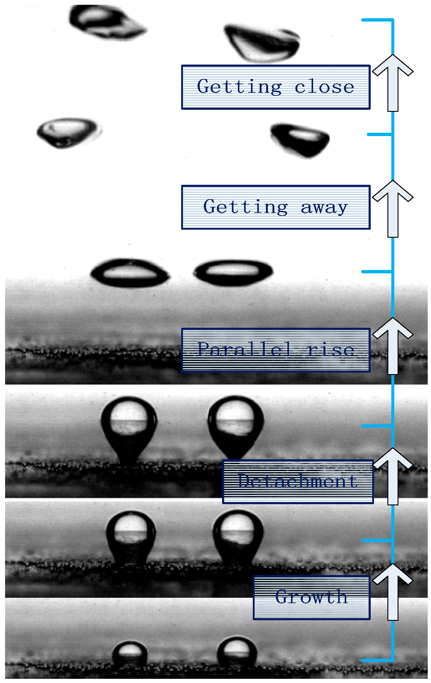
Under the condition that the orifice diameter was 2 mm, gas flow rate was 40 mL/min, and the orifice spacing was d = 8 mm; the rising process of bubbles was shot and tracked. Based on the change law of bubbles, the formation and movement process was divided into five stages (growth, detachment, parallel rise, getting away, and getting close), as shown in Figure 6.
At the growth stage, the bubble radius increased rapidly based on orifice size. The bubble mainly grew along the Y-axis direction and was stretched lengthwise due to the impact of the gas. Under the action of surface tension, the bubble gradually grew into a smooth ellipsoid shape. When the bubbles grew, the abscissa of bubbles’ centers of mass remained unchanged, and the velocity of the bubble in the horizontal direction was approximately zero. Since the volume of the bubble increased, however, the position of the center of mass of the bubble moved up, resulting in a small upward velocity of the center of mass, as shown in Figure 7.
At the separation stage, the bubble necks and the contact area with the wall gradually decreased and the abscissa of the bubble center of mass still remained unchanged. However, the longitudinal velocity increased rapidly, and the bubble reached about 50% of the final stable velocity at the moment of separation. After the bubbles left the wall, two bubbles rose in parallel form. Due to the separation of bubble and porosity, the impact of the gas disappeared; bubbles needed to change shape to meet the new force equilibrium, and the energy for the bubble deformation was from the previous kinetic energy of bubbles, as shown in Figure 7, the considerable deformation of bubbles made the velocity of rising bubbles sharply and significantly decrease, and finally, bubbles became spheroid, as shown in Figure 6. The bubbles maintained the same distance between the center of mass, but the minimum distance between bubbles decreased obviously.
Figure 8 shows the lateral velocity variation law with time. As can be seen, the transverse velocity of the bubbles approximately represents simple harmonic oscillation: the bubbles always moved in the opposite direction. When the distance between the bubbles became smaller, they attempted to repel and move away from each other. The two bubbles changed their movement direction and velocity, and they approached after reaching the farthest distance.
After the parallel rising stage, the rising trajectory of bubbles was not linear, but there was oscillation to left and right at the same time. A cycle of approaching, leaving, and then approaching occurred. Figure 9 shows the rising trajectory of the two bubbles.
4.1.2. Effect of Different Intake Conditions on Bubble Characteristics
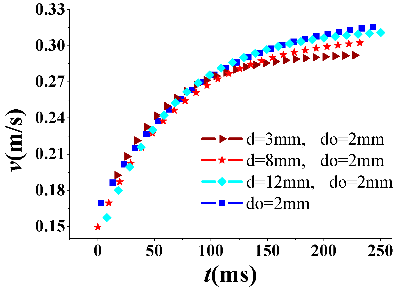
When the diameter of the orifice was 2 mm, the bubble characteristics of different flow rates under four conditions (orifice spacing of d = 3 mm, 8 mm and 12 mm, and single orifice) were studied throughout the experiment. Figure 10 shows the change regulation of bubble velocity over time under different orifice spacing condition. It can be found that bubble velocity variation showed almost the same change trend; The final stable velocity of bubbles under different orifice spacing was slightly different, and they still showed a certain regularity: when the gas flow rate and orifice size remained the same, the smaller the orifice spacing was, the smaller final stable velocity bubbles had.
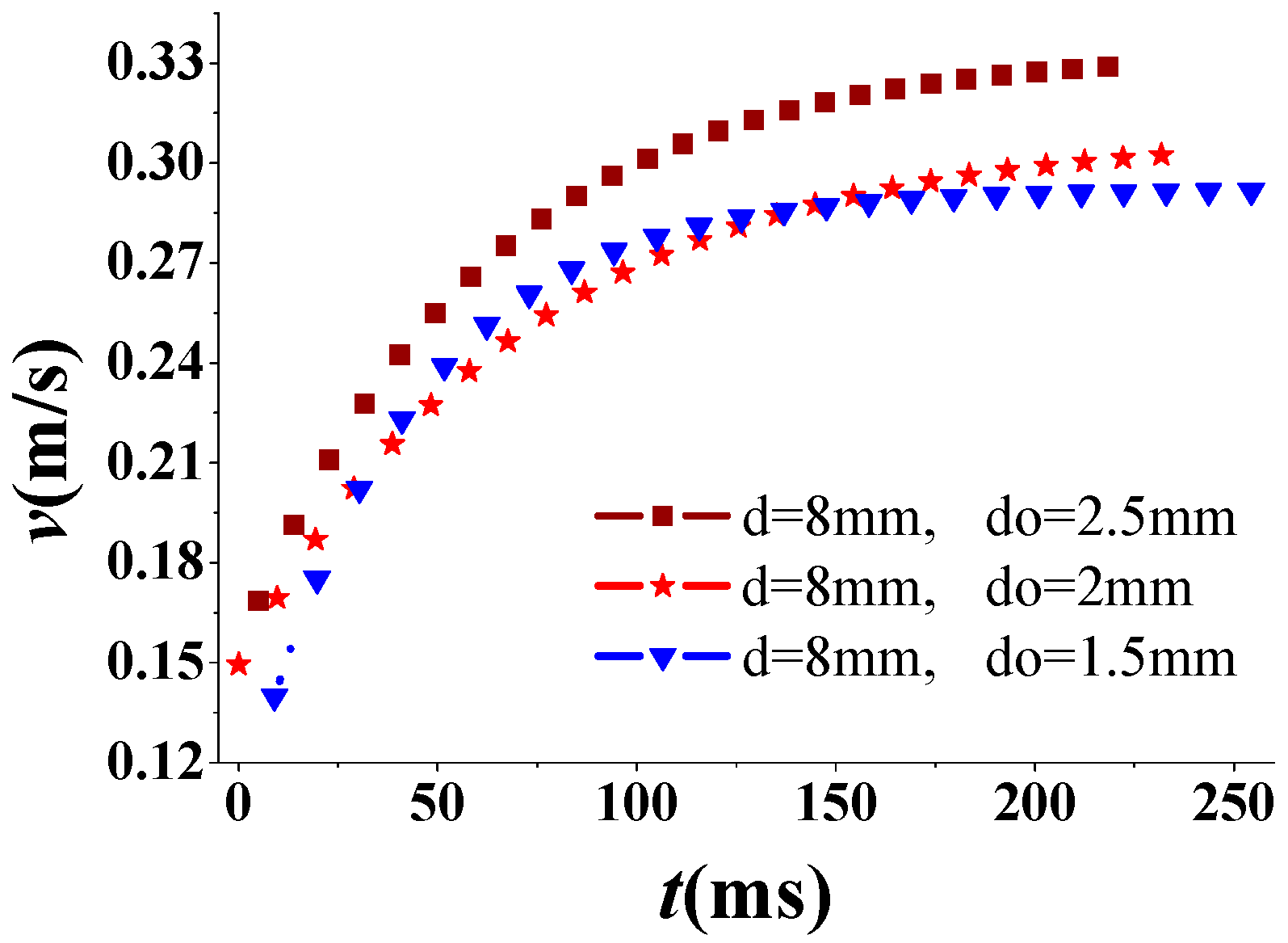
When orifice spacing was 8 mm, the bubble characteristics of different flow rates under three conditions (diameter of orifice: d = 3 mm, 8 mm and 12 mm) were studied through experiment. Moreover, the bubble size at detachment under the three conditions were extracted. Figure 11 shows the change law of bubble rising velocity with time under different hole sizes. It was found that the change trend of bubble velocity was the same as that described above, and when the gas flow rate and orifice spacing remained the same, the smaller the orifice size was, the smaller final stable velocity bubbles had. According to the Stokes’s theory, it can be seen that the final velocity of the bubble was related to the size of the bubble, the smaller the orifice size was, the smaller the bubble size would be, which would slow down the final velocity of the bubble.
4.2. Experimental Validation of the Numerical Model
Figure 12 shows the rising trajectory of bubbles obtained from simulation. As can be seen, the simulation results were in good agreement with bubbles’ movement tracks throughout the experiment, and there was a cycle of approaching, leaving, and then approaching. Furthermore, according to Figure 12, the minimum distance that bubbles reached at the approaching stage was greater than the previous one, and the maximum distance was larger than the previous one. Thereby, the bubbles were gradually separated when they were accompanied by a cycle of approaching, leaving, and then approaching.
Figure 13a shows the change process of the relationship between the positions of the two bubbles obtained by simulation. The eight groups of data from bottom to top are the positions of the bubbles at time t = 0.05 s, 0.09 s, 0.13 s, 0.17 s, 0.21 s, 0.25 s, 0.29 s, and 0.33 s. Figure 13b shows the data of the shot image, and it shows the changes rule of the relative position and shape of two bubbles separated at the same time, with time in the rising process. It was found that the simulation results framed by solid line were consistent with the results observed in the experiment. The two bubbles presented the cycling phenomenon of “V” shape and inverted “V” shape in the rising process.
4.3. Numerical Simulation Results
Bubbles have certain effects on water disturbance range. When two bubbles move together, interaction is produced only when the bubble is located in the influence range of another bubble, causing the change of the surrounding flow field structure. Then, the shape and upward trajectory change, and even collision and aggregation phenomena appear. This paper only studied the movement characteristics of two bubbles in view of the horizontal distribution rising side by side in quiescent water and did not consider the collision and aggregation process.
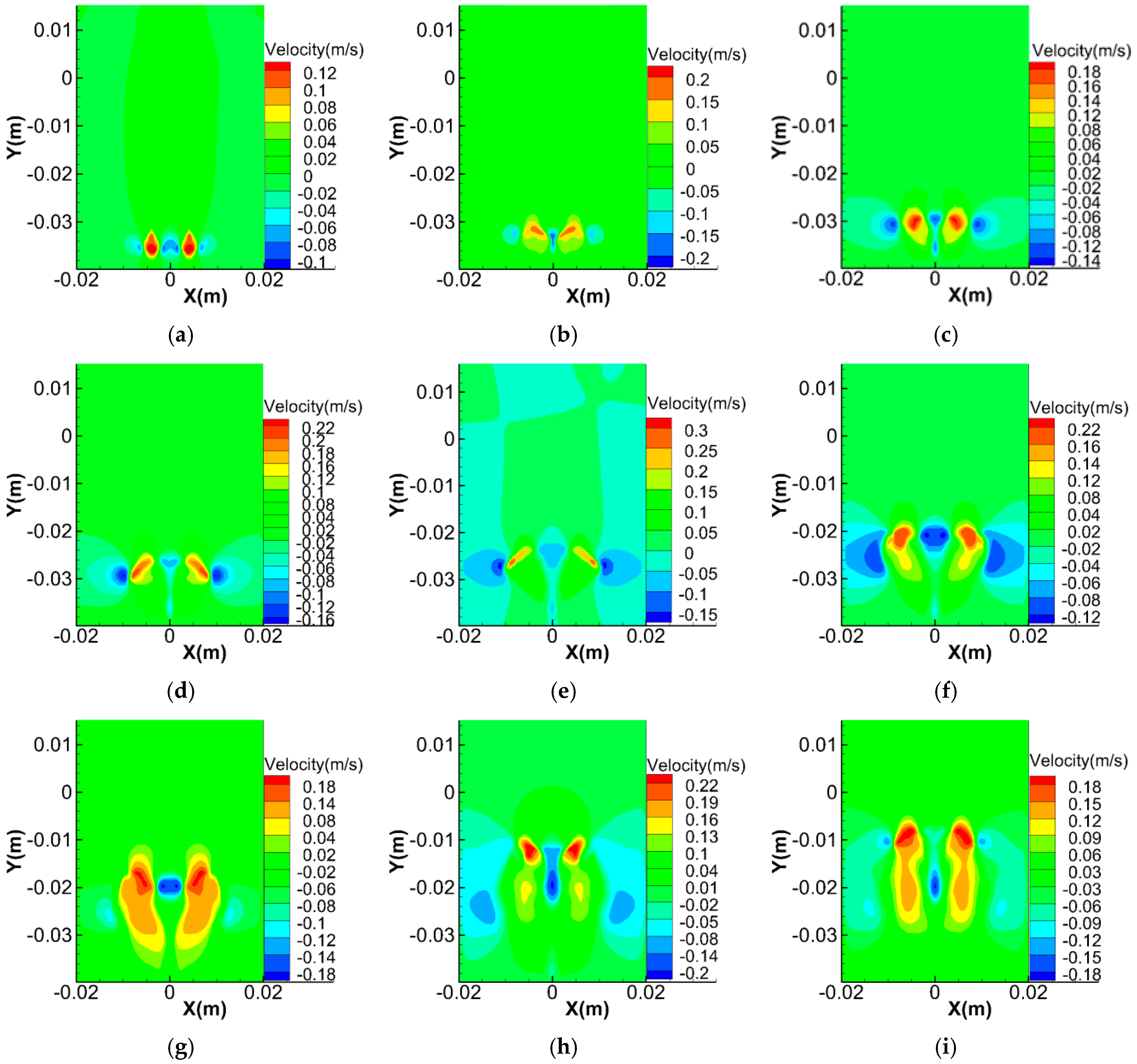
Figure 14 shows the deformation process and the flow field structure of the two bubbles. As can be observed, the two bubbles formed the flow fields with symmetrical distribution in the process of movement, which was characterized by a jet at the bottom of each bubble and a similar circular flow field structure on both sides of each bubble. Furthermore, both sides of the flow field rotated in opposite directions. To be specific, the flow field around the left side of bubbles rotated counterclockwise, while that around the right side rotated clockwise.
Bubbles had weak mutual influence at the initial stage. As the bubbles gradually became flat, there was less distance between them, and mutual influence became stronger. A layer of liquid membrane formed between the bubbles and the flow inside the liquid membrane was under the influence of two bubbles at the same time. The flow field of the liquid membrane region can be thought of as superposition of the two-flow field generated by the bubble disturbance around, as shown in Figure 15. It was found that the fluid in the liquid membrane dropped faster than the other two sides. A low-pressure area was produced, and the two bubbles attracted each other when rising, as shown in Figure 14b.
At the same time, because the horizontal velocity of the flow field generated by the two bubbles in the liquid membrane region was opposite, the action point of the jet generated by the flow field at the bottom of the two bubbles moved towards the liquid membrane region. The part of the bubbles located at the side of the liquid membrane was subjected to large jet thrust and rose relatively quickly. The two bubbles rotated due to unbalanced forces on both sides, and they were distributed in an inverted “V” shape (Figure 14d). The impelling effect of the jet on the bubbles was greater than that of the middle low-pressure area. The bubbles gradually moved away from each other, and their influence on each other became smaller. The horizontal velocity offset effect of the flow field generated by the two bubbles in the liquid membrane region became smaller. The action point of the jet on the bubbles moved towards the center of the bubbles, as shown in Figure 14e.
At the same time, the part of the two bubbles near the wall surface moved behind, were at the deeper water level position, and had greater pressure. Thus, the air here moved towards the low-pressure area (i.e., the position of the shallow water level) inside the bubbles. The shape and position of the two bubbles were in an approximately horizontal state after a period of time, as shown in Figure 14f. As a result of the movement of air in bubbles to the middle area and a smaller distance between the bubbles, the drop velocity of fluid in the middle became larger, and a low-pressure area formed. Thus, the two bubbles noticeably attracted each other. As seen from Figure 15e, when the two bubbles left, the liquid membrane thickened; when the two bubbles approached again, they entered the liquid membrane region and the liquid membrane fluid flowed downward to the inside. The bubbles were distributed in a “V” shape when they approached each other (Figure 14g).
Due to the small distance between the bubbles, the liquid flow field superposition effect generated by the two bubbles in the membrane region was obvious; the action point of the bubble tail jet on bubbles moved to the liquid membrane region once again. Due to the thrust effect of water flow, the velocity of the part of bubbles in the liquid membrane region increased gradually and the bubble shape and position were in a horizontal state again. Then, the two bubbles got close, got away, and got close, and such a movement process was accompanied by the circulation phenomenon of two bubbles distributed in a “V” shape and inverted “V” shape.
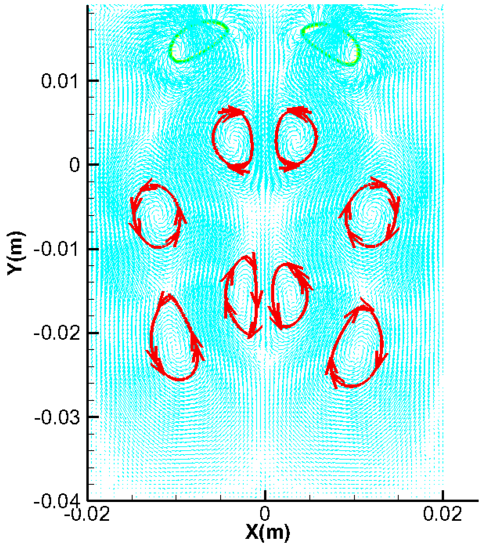
The unbalanced forces on the left and right part of the two bubbles in the rising process caused whirlpools in the surrounding fluid after bubble disturbance. Figure 16 shows the flow field structure in the pipeline when t = 0.4 s. The position relationship of bubbles went through two cycles within the period of 0.4 s, and two pairs of whirlpools were generated in each cycle.
5. Conclusions
In this paper, numerical simulation and visualization experiments are carried out on the motion characteristics of two bubbles rising side by side. After analyzing the movement trajectory, shape change, and horizontal and vertical velocity change rules of bubbles, the following conclusions are drawn:
- (1)
- When two bubbles rose side by side, their rising trajectory was not vertical, moved laterally, and showed a cycle process of approaching, leaving, and then approaching. In addition, in this cycle process, the horizontal velocity of the bubbles changed in a simple harmonic law, and the movement direction of the left bubble and right bubble was always opposite.
- (2)
- In the case of the same orifice spacing and gas flow rate, the greater the orifice size was, the greater final stable velocity bubbles had, and in the case of the same orifice size and gas flow rate, the smaller the orifice spacing was, the smaller final stable velocity bubbles had.
- (3)
- Both numerical and experimental studies have found that in the process of rising, the relative location of the two bubbles is present cycle changes of “V” shape and inverted “V” shape, the simulation results are quite consistent with the phenomenon observed through experiment, so the proposed mathematical model is compatible with the experiment.
- (4)
- From the numerical results, it is concluded that when two bubbles rise side by side, each bubble rises in the form of an up and down swing, which causes whirlpools in the surrounding water. During a period when the bubble position relationship changes, there are two pairs of whirlpools at the tail of the two bubbles.
By employing visual experiments and numerical simulation, we attempt here to study the motion of two bubbles rising side by side; the calculated values have good consistency with the experimental results. However, the bubbles would not stay in a vertical plane the entire time during the experiment, so in the future work, more simulations in 3D are planned in order to improve the accuracy and reliability of numerical model. An insight into the physics of the process also will be carried out in the future, such as the variation to the number of Reynolds for bubble wake area, and the variation to the numbers Eötvös and Tadaki in the process of bubble deformation.
Author Contributions
This work was done by all of the authors. The manuscript was written by the first author.
Funding
This research was funded by National Natural Science Foundation of China (No.11605033) and the LLOYD’S REGISTER FOUNDATION.
Acknowledgements
The authors greatly appreciate the support of Fundamental Science on Nuclear Safety and Simulation Technology Laboratory, Harbin Engineering University, College of Nuclear Science and Technology, China. The authors wish to thank the National Natural Science Foundation of China (No.11605033) and the LLOYD’S REGISTER FOUNDATION for financial support. The LLOYD’S REGISTER FOUNDATION is an independent charity, working to achieve advances in transportation, science, engineering, and technology education, and training and research worldwide for the benefit of all.
Conflicts of Interest
The authors declare no conflict of interest.
References
- Xie, Y.B.; Liu, D.P.; Yang, L.; Yang, M. Experimental study on the growth characteristics of natural gas hydrate formation on suspended gas bubbles in distilled water and tap water. Chem. Ind. Eng. Prog. 2017, 36, 129–135. [Google Scholar]
- Yang, H.; Zhu, C.Y.; Ma, Y.G.; Gao, X.Q. Continuous formation and coalescence of bubbles through double-nozzle in non-Newtonian fluid. Chem. Eng. 2016, 44, 37–41. [Google Scholar]
- Painmanakul, P.; Loubiere, K.; Hebrard, G.; Buffière, P. Study of different membrane spargers used in waste water treatment: Characterisation and performance. Chem. Eng. Process. 2004, 43, 1347–1359. [Google Scholar] [CrossRef]
- Gnyloskurenko, S.V.; Byakova, A.V.; Raychenko, O.I.; Nakamura, T. Influence of wetting conditions on bubble formation at orifice in an inviscidliquid. Physicochem. Eng. Asp. 2003, 218, 73–87. [Google Scholar] [CrossRef]
- Chen, D.Q.; Pan, L.M.; Ren, S. Prediction of bubble detachment diameter in flow boiling based on force analysis. Nucl. Eng. Des. 2012, 243, 263–271. [Google Scholar] [CrossRef]
- Peter, M.W.; Antoinet, V.S.; Josette, P.M.S. The influence of gas density and liquid properties on bubble breakup. Chem. Eng. Sci. 2012, 48, 1213–1226. [Google Scholar]
- Pan, L.M.; Tan, Z.W.; Chen, D.Q.; Xue, L.C. Numerical investigation of vapor bubble condensation characteristics of subcooled flow boiling in vertical rectangular channel. Nucl. Eng. Des. 2012, 248, 126–136. [Google Scholar] [CrossRef]
- Zhang, L.; Yang, C.; Mao, Z.S. Numerical simulation of a bubble rising in shear-thinning fluids. J. Non-Newton. Fluid Mech. 2010, 165, 555–567. [Google Scholar] [CrossRef] [Green Version]
- David, F.F.; Brian, S.H. Validation of a CFD model of Taylor flow hydrodynamics and heat transfer. Chem. Eng. Sci. 2012, 69, 541–552. [Google Scholar]
- Wittke, D.D.; Chao, T.B. Collapse of vapor bubbles with translatory motion. J. Heat Transf. 1967, 89, 17–24. [Google Scholar] [CrossRef]
- Choi, H.M.; Terauchi, T.; Monji, H.; Matsui, G. Visualization of bubble-fluid interaction by a moving object flow image analyzer system. Ann. N. Y. Acad. Sci. 2002, 972, 235–241. [Google Scholar] [CrossRef]
- Zhu, X.; Xie, J.; Liao, Q. Dynamic bubbling behaviors on a micro-orifice submerged in stagnant liquid. Int. J. Heat Mass Transf. 2014, 68, 324–331. [Google Scholar] [CrossRef]
- Ngoh, J.; Lim, E.W.C. Effects of particle size and bubbling behavior on heat transfer in gas fluidized beds. Appl. Ther. Eng. 2016, 105, 225–242. [Google Scholar] [CrossRef]
- Cano-Pleite, E.; Hernández-Jiménez, F.; de Vega, M.; Acosta-Iborra, A. Experimental study on the motion of isolated bubbles in a vertically vibrated fluidized bed. Chem. Eng. J. 2014, 255, 114–125. [Google Scholar] [CrossRef]
- Gnyloskurenko, S.; Byakova, A.; Nakamura, T.; Raychenko, O. Influence of wettability on bubble formation in liquid. J. Mater. Sci. 2005, 40, 2437–2441. [Google Scholar] [CrossRef]
- Sagert, N.H.; Quinn, M.J. Influence of high- pressure gases on the stability of thin aqueous films. J. Colloid Interface Sci. 1977, 61, 279–286. [Google Scholar] [CrossRef]
- Lau, R.; Mo, R.; Beverly, W.S. Bubble characteristics in shallow bubble column reactors. Chem. Eng. Res. Des. 2010, 88, 197–203. [Google Scholar] [CrossRef]
- Ribeiro Jr, C.P.; Lage, P.L.C. Experimental study on bubble size distributions in a direct-contact evaporator. Braz. J. Chem. Eng. 2004, 21, 69–81. [Google Scholar] [CrossRef] [Green Version]
- Aladjem, T.C.; Shemer, L.; Barnea, D. On the interaction between two consecutive elongated bubbles in a vertical pipe. Int. J. Multiph. Flow 2000, 26, 1905–1923. [Google Scholar] [Green Version]
- Liao, Y.X.; Roland, R.; Dirk, L. Baseline closure model for dispersed bubbly flow: Bubble coalescence and breakup. Chem. Eng. Sci. 2015, 122, 336–349. [Google Scholar] [CrossRef]
- Zuzana, B.; Thodoris, K.; Margaritis, K. Bubble–particle collision interaction in flotation systems. Colloids Surf. A Physicochem. Eng. Asp. 2015, 473, 95–103. [Google Scholar]
- Vélez-Cordero, J.R.; Sámano, D.; Yue, P.; Feng, J.J.; Zenit, R. Hydrodynamic interaction between a pair of bubbles ascending in shear-thinning inelastic fluids. J. Non-Newton. Fluid Mech. 2011, 166, 118–132. [Google Scholar] [CrossRef]
- Hallez, Y.; Legendre, D. Interaction between two spherical bubbles rising in a viscous liquid. J. Fluid Mech. 2011, 673, 406–431. [Google Scholar] [CrossRef] [Green Version]
- Costigan, G.; Whalley, P.B. Measurements of the speed of sound in air-water flows. Chem. Eng. J. 1997, 66, 131–135. [Google Scholar] [CrossRef]
- Thoroddsen, S.T.; Etoh, T.G.; Takehara, K. High-speed imaging of drops and bubbles. Annu. Rev. Fluid Mech. 2008, 40, 257–285. [Google Scholar] [CrossRef]
- Muller, R.L.; Prince, R.G.H. Regimes of bubbling and jetting from submerged orifices. Chem. Eng. Sci. 1972, 27, 1583–1592. [Google Scholar] [CrossRef]
- Monica, M.; Cushman, J.H.; Cenedese, A. Application of photogrammetric 3D-PTV Technique to track particles in porous media. Transp. Porous Media 2009, 79, 43–65. [Google Scholar] [CrossRef]
- Xue, T.; Xu, L.S.; Zhang, S.Z. Bubble behavior characteristics based on virtual binocular stereo vision. Optoelectron. Lett. 2018, 14, 95–103. [Google Scholar] [CrossRef]
- Belden, J.; Ravela, S.; Truscott, T.T.; Techet, A.H. Three-dimensional bubble field resolution using synthetic aperture imaging: Application to a plunging jet. Exp. Fluids 2012, 53, 839–869. [Google Scholar] [CrossRef]
- Stewart, C.W. Bubble interaction in low-viscosity liquids. Int. J. Multiph. Flow 1995, 21, 1037–1046. [Google Scholar] [CrossRef]
- Brucker, C. Structure and dynamics of the wake of bubbles and its relevance for bubble interaction. Phys. Fluids 1995, 11, 1781–1796. [Google Scholar] [CrossRef]
- Dong, Z.; Li, W.; Song, Y. A numerical investigation of bubble growth on and departure from a superheated wall by lattice Boltzmann method. Int. J. Heat Mass Transf. 2010, 53, 4908–4916. [Google Scholar] [CrossRef]
- Zhang, Z.Y.; Jin, L.A.; He, S.Y.; Yuan, Z.J. Study on coupling models for bubble floatation accompanied with heat and mass transfer. J. Chem. Eng. Chin. Univ. 2018, 32, 358–367. [Google Scholar]
- Yoo, D.H.; Tsuge, H.; Terasaka, K.; Mizutani, K. Behavior of bubble formation in suspended solution for an elevated pressure system. Chem. Eng. Sci. 1997, 52, 3701–3707. [Google Scholar] [CrossRef]
- Ding, Y.D.; Liao, Q.; Zhu, X.; Wang, H.; Liu, Z.H. Characteristics of bubble growth and water invasion at the permeable sidewall in rectangular liquid flow channel. J. Mech. Eng. 2013, 49, 119–124. [Google Scholar] [CrossRef]
- Du, Y.H.; Xiong, K.W.; Zhang, Y.; Nie, X.T.; Zhou, M.; Li, C.B. Analysis of numerical simulation on horizontal arrangement equal bubbles rising. Chin. J. Comput. Mech. 2016, 33, 889–894. [Google Scholar]
- Li, Y.; Zhang, J.P.; Fan, L.S. Discrete-phase simulation of single bubble rise behavior at elevated pressures in a bubble column. Chem. Eng. Sci. 2000, 55, 4597–4609. [Google Scholar] [CrossRef]
- Li, Y.; Zhang, J.P.; Fan, L.S. Numerical studies of bubble dynamics in gas-liquid-solid fluidization at high pressures. Power Technol. 2001, 116, 246–260. [Google Scholar] [CrossRef]
- Yang, G.Q.; Du, B.; Fan, L.S. Bubble formation and dynamics in gas-liquid-solid fluidization—A review. Chem. Eng. Sci. 2007, 62, 2–27. [Google Scholar] [CrossRef]
- Zhang, J.P.; Li, Y.; Fan, L.S. Numerical studies of bubble and particle dynamics in a three-phase fluidized bed at elevated pressures. Powder Technol. 2000, 112, 46–56. [Google Scholar] [CrossRef]
- Hua, J.S.; Lin, P.; Jan, F.S. Numerical simulation of gas bubbles rising in viscous liquids at high Reynolds number. Contemp. Math. 2008, 466, 1–18. [Google Scholar]
- Chen, L.; Li, Y. A numerical method for two-phase flows with an interface. Environ. Model Softw. 1998, 13, 247–255. [Google Scholar] [CrossRef]
- Yang, S.M.; Tao, W.Q. Heat Transfer, 4th ed.; Higher Education Press: Beijing, China, 2007; pp. 559–563. [Google Scholar]
- Brackbill, J.U.; Kothe, D.B.; Zemach, C. A contiuum method for modeling surface tension. J. Comput. Phys. 1992, 100, 335–354. [Google Scholar] [CrossRef]
- Kok, J.B.W. Dynamics of gas bubbles moving through liquid: Part I: Theory. Eur. J. Mech. 1993, B12, 515–540. [Google Scholar]
- Kok, J.B.W. Dynamics of gas bubbles moving through liquid: Part II: Experiments. Eur. J. Mech. 1993, B12, 541–560. [Google Scholar]
- Vries, A.W.G.; Biesheuvel, A.; Wijingaarden, L. Notes on the path and wake of a gas bubble rising in pure water. Int. J. Multiph. Flow 2002, 28, 1823–1835. [Google Scholar] [CrossRef]
- Sanada, T.; Sato, A.; Shirota, M.; Watanabe, M. Motion and coalescence of a pair of bubbles rising side by side. Chem. Eng. Sci. 2009, 64, 2659–2671. [Google Scholar] [CrossRef] [Green Version]
Figure 1.
Study of grid independence on the simulated bubble.

Figure 2.
Experimental device and system: (1) water tank; (2) bubble generation module; (3) LED plane light source; (4) check valve; (5) float flow meter; (6) air pump; (7) high-speed camera; (8) computer.
Figure 2.
Experimental device and system: (1) water tank; (2) bubble generation module; (3) LED plane light source; (4) check valve; (5) float flow meter; (6) air pump; (7) high-speed camera; (8) computer.

Figure 3.
Bubble generation module.

Figure 4.
Area of interest (AOI) of bubble: (a) Photograph taken by high speed camera; (b) Image processed by Image-Pro Plus (IPP) software.
Figure 4.
Area of interest (AOI) of bubble: (a) Photograph taken by high speed camera; (b) Image processed by Image-Pro Plus (IPP) software.

Figure 5.
Bubble parameter calculation method.

Figure 6.
Five stages of two bubbles’ formation and movement.

Figure 7.
Longitudinal velocity versus time.
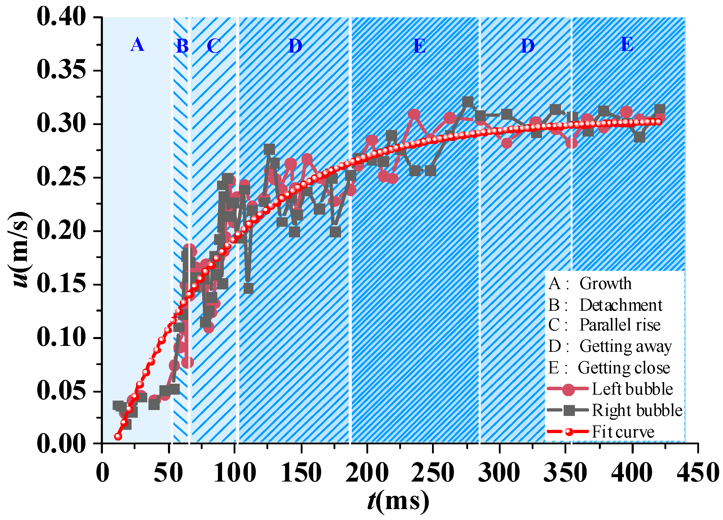
Figure 8.
Lateral velocity versus time.

Figure 9.
Bubble rising trajectory.
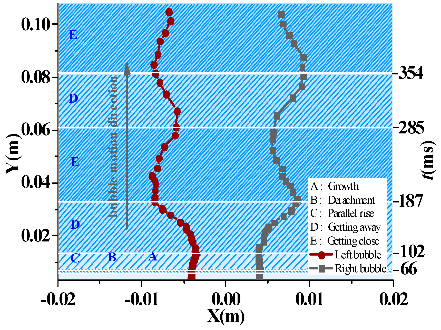
Figure 10.
Velocity variation with time under different conditions.

Figure 11.
Velocity variation with time under different conditions.

Figure 12.
Bubble rising trajectory obtained from simulation.
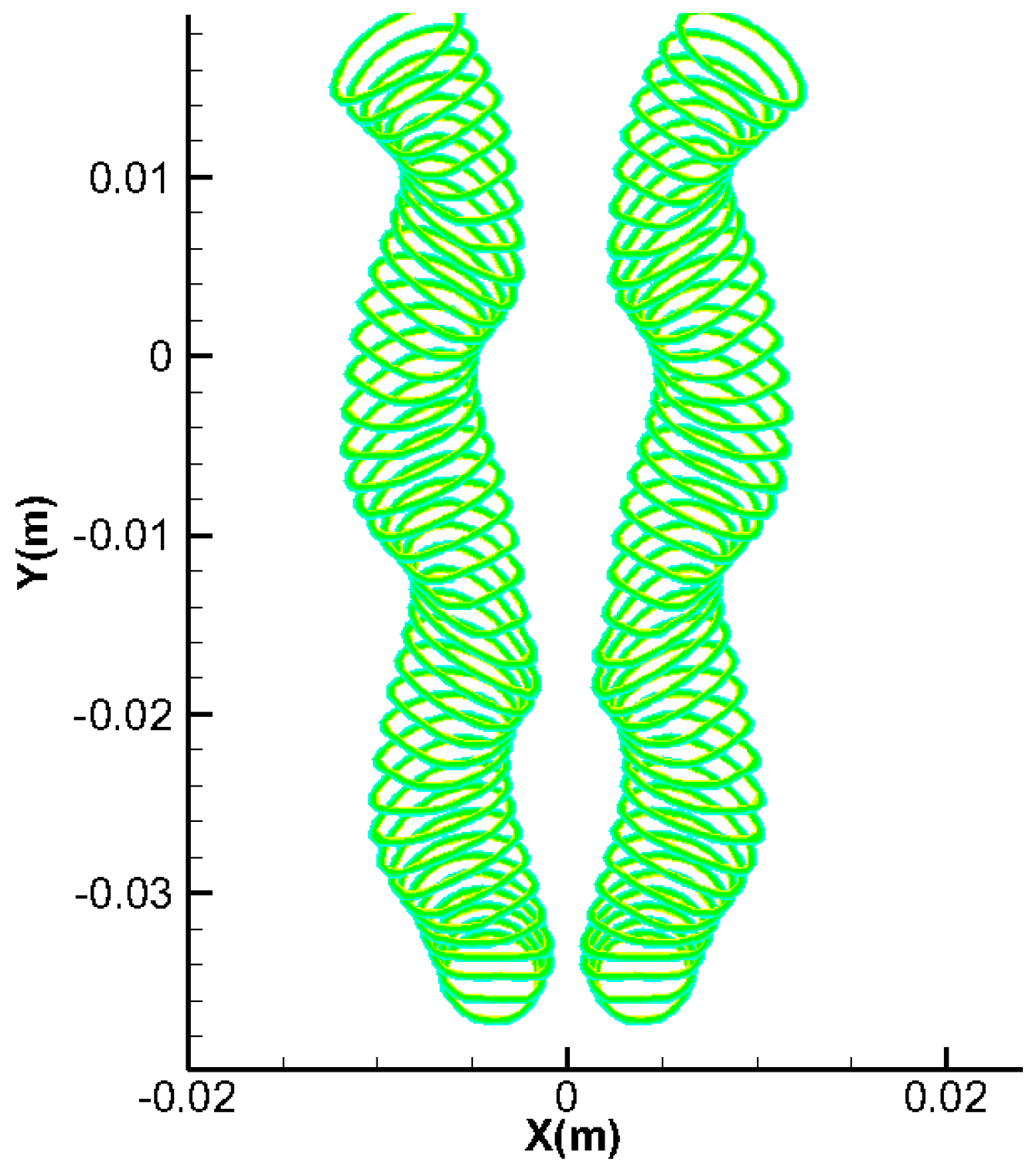
Figure 13.
The cyclicity of position relations between two rising bubbles: (a) Result obtained by simulation; (b) Result obtained by experiment.
Figure 13.
The cyclicity of position relations between two rising bubbles: (a) Result obtained by simulation; (b) Result obtained by experiment.
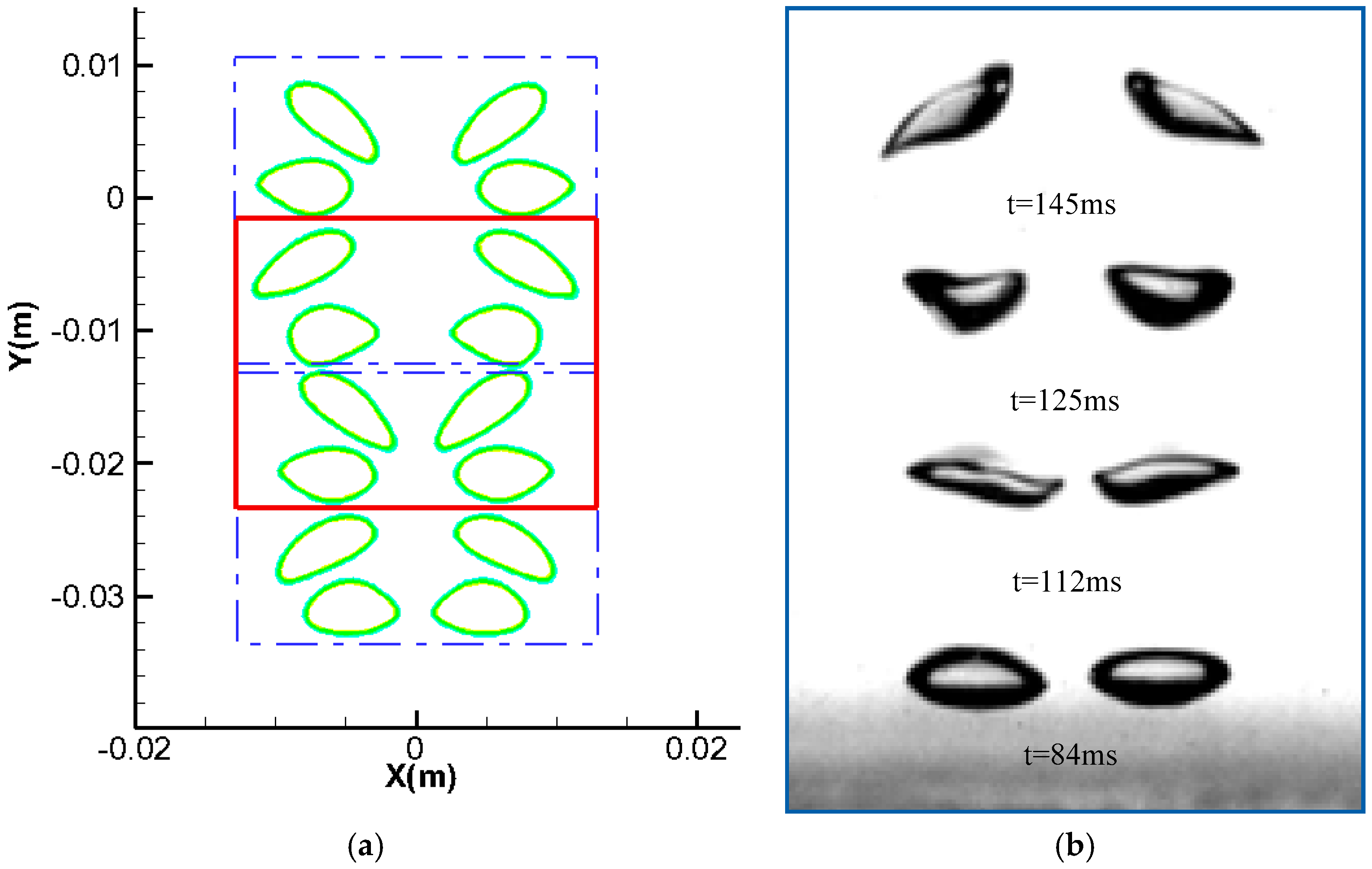
Figure 14.
The Streamline shape and deformation process of two rising bubble. (a) t = 0.01 s; (b) t = 0.04 s; (c) t = 0.06 s; (d) t = 0.08 s; (e) t = 0.1 s; (f) t = 0.13 s; (g) t = 0.15 s; (h) t = 0.20 s; (i) t = 0.22 s.
Figure 14.
The Streamline shape and deformation process of two rising bubble. (a) t = 0.01 s; (b) t = 0.04 s; (c) t = 0.06 s; (d) t = 0.08 s; (e) t = 0.1 s; (f) t = 0.13 s; (g) t = 0.15 s; (h) t = 0.20 s; (i) t = 0.22 s.
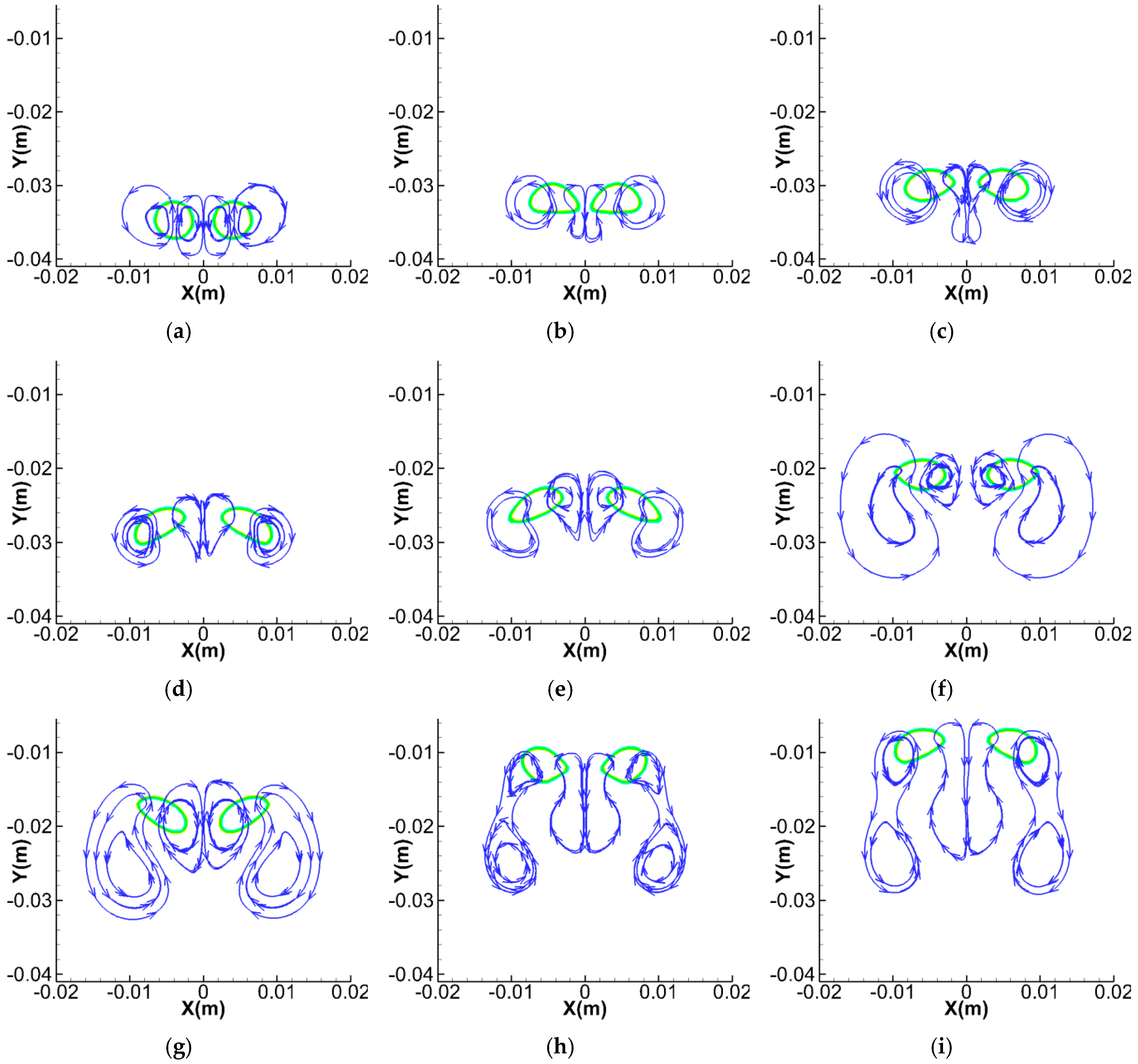
Figure 15.
The velocity distribution of two rising bubbles. (a) t = 0.01 s; (b) t = 0.04 s; (c) t = 0.06 s; (d) t = 0.08 s; (e) t = 0.1 s; (f) t = 0.13 s; (g) t = 0.15 s; (h) t = 0.20 s; (i) t = 0.22 s.
Figure 15.
The velocity distribution of two rising bubbles. (a) t = 0.01 s; (b) t = 0.04 s; (c) t = 0.06 s; (d) t = 0.08 s; (e) t = 0.1 s; (f) t = 0.13 s; (g) t = 0.15 s; (h) t = 0.20 s; (i) t = 0.22 s.

Figure 16.
The vortex generated by a rising bubble.


Table 1.
The physical parameters.
| Air Density | Water Density | Air Viscosity | Water Viscosity | Surface Tension | Morton Number |
|---|---|---|---|---|---|
| (kg/m3) | (kg/m3) | (Pa·s) | (Pa·s) | (N/m) | Mo |
| 1.225 | 988.2 | 1.7894 × 10⁻⁵ | 0.001 | 0.074 | 3.14 × 10⁻¹¹ |
© 2019 by the authors. Licensee MDPI, Basel, Switzerland. This article is an open access article distributed under the terms and conditions of the Creative Commons Attribution (CC BY) license (http://creativecommons.org/licenses/by/4.0/).
Share and Cite
MDPI and ACS Style
Ying, H.; Puzhen, G.; Chaoqun, W. Experimental and Numerical Investigation of Bubble–Bubble Interactions during the Process of Free Ascension. Energies 2019, 12, 1977. https://doi.org/10.3390/en12101977
AMA Style
Ying H, Puzhen G, Chaoqun W. Experimental and Numerical Investigation of Bubble–Bubble Interactions during the Process of Free Ascension. Energies. 2019; 12(10):1977. https://doi.org/10.3390/en12101977
Chicago/Turabian StyleYing, Huang, Gao Puzhen, and Wang Chaoqun. 2019. "Experimental and Numerical Investigation of Bubble–Bubble Interactions during the Process of Free Ascension" Energies 12, no. 10: 1977. https://doi.org/10.3390/en12101977
Note that from the first issue of 2016, this journal uses article numbers instead of page numbers. See further details here.