An Analytical Model for Capturing the Decline of Fracture Conductivity in the Tuscaloosa Marine Shale Trend from Production Data


Department of Petroleum Engineering, University of Louisiana at Lafayette, Lafayette, LA 70504, USA
*
Authors to whom correspondence should be addressed.
Energies 2019, 12(10), 1938; https://doi.org/10.3390/en12101938
Submission received: 26 February 2019
/
Revised: 9 May 2019
/
Accepted: 17 May 2019
/
Published: 21 May 2019
(This article belongs to the Section L: Energy Sources)
Abstract
:Fracture conductivity decline is a concern in the Tuscaloosa Marine Shale (TMS) wells due to the high content of clay in the shale. An analytical well productivity model was developed in this study considering the pressure-dependent conductivity of hydraulic fractures. The log-log diagnostic approach was used to identify the boundary-dominated flow regime rather than the linear flow regime. Case studies of seven TMS wells indicated that the proposed model allows approximation of the field data with good accuracy. Production data analyses with the model revealed that the pressure-dependent fracture conductivity in the TMS in the Mississippi section declines following a logarithmic mode, with dimensionless coefficient χ varying between 0.116 and 0.130. The pressure-dependent decline of fracture conductivity in the transient flow period is more significant than that in the boundary-dominated flow period.
1. Introduction
The Tuscaloosa Marine Shale (TMS) across Louisiana and Mississippi has been an attractive unconventional shale oil reservoir since 2012 [1]. The TMS is a sedimentary formation that consists of organic-rich fine-grained sediments deposited during the Upper Cretaceous [2]. The TMS is one part of the Tuscaloosa group consisting of Upper Tuscaloosa, Middle Marine Shale, and Lower Tuscaloosa [3]. The thickness of TMS ranges from 500 ft in the southwestern Mississippi to more than 800 ft in southeastern Louisiana, within a depth range of 11,000 to more than 15,000 ft [4]. Middle Tuscaloosa is composed of a dark grey, fissile, and sandy marine shale. Experimental results indicated that the permeability ranges from less than 0.01 to 0.06 md, and porosity ranges from 2.3% to 8.0% [4].
More than 80 multi-fractured horizontal wells were drilled in the TMS between 2012 and 2014 [2]. Several TMS wells were recorded to have appealing initial oil production rates exceeding 1000 stb/d. Although such significant high production rates were observed, drilling activities stopped in 2014 due to the high cost of drilling and low price of oil. Previous studies estimated an unproven recoverable oil of seven billion barrels [4], but the real production potential from TMS is still poorly understood. It is of significance to assess the TMS well performance through production decline analysis and identify key factors controlling the productivity of TMS wells.
Mathematical modeling plays an important role in analyzing well behavior and identifying factors that affected well performance in the past. The available models for predicting shale oil well long-term productivity include (1) analytical transient flow models [5,6,7], (2) numerical computer models [8,9,10], and (3) empirical production decline models [11,12,13,14,15]. The analytical transient flow models are utilized in pressure transient test analysis rather than in production data analysis. Although numerical computer models are flexible in handling systems with non-symmetrical fractures and multiphase flow, applications of these models are limited owing to the low efficiency of their numerical nature, especially the numerical treatment of local grid refinement near the fractures. Uncertainty in locations of natural fractures is another concern regarding the accuracy of the computer simulation result. The empirical production decline models were not derived based on engineering principles. They are mainly utilized for evaluating field development projects on the basis curve fitting to the production history data [16]. Besides, empirical production decline models are mostly applicable to boundary-dominated flow conditions that are often the case for conventional reservoirs. Wells in unconventional reservoirs are characterized by long-term transient flow owing to ultra-low reservoir permeability [17,18]. These models are not suitable for evaluating the real potential and identifying factors controlling the potential of TMS wells.
Hydraulic fracture conductivity plays an essential role in well performance [19,20,21,22,23,24]. It can decline significantly during production owing to proppant embedment and blockage of debris [25,26]. Experimental investigations have indicated that hydraulic fracture conductivity declines logarithmically or exponentially with time [27,28]. Sun et al. [28] demonstrated that the decrease in fracture conductivity could reduce the production decline curve value and lead to a significant production drop. Production decline analysis failing to take time-dependent fracture conductivity into account will lead to significant errors in production prediction of multi-fractured wells in unconventional shale reservoirs.
Fracture conductivity declines exponentially in the Haynesville Shale, which is very close to the TMS [29]. The decline in TMS is of particular concern because of the high level of clay materials in TMS [2]. Clay minerals are water-sensitive, making the fracture face soft and vulnerable to the embedment of fracture proppant, leading to a fracture conductivity drop due to partial closure of the fracture. This study focuses on capturing the pressure-dependent decline rate of fracture conductivity in TMS wells under the boundary-dominated flow conditions using production data. An analytical well productivity model was developed in this study considering time-dependent fracture conductivity. Case studies of seven TMS wells indicate that the production rates calculated by the analytical model agree with field data very well. Production data analyses with the model revealed that fracture conductivity in the TMS in the Mississippi section declines following a logarithmic mode.
2. Mathematical Model
An analytical model was developed in this work for capturing the decline of pressure-dependent fracture conductivity of multi-fractured shale oil wells under boundary-dominated flow conditions. The assumptions on the analytical model include the following,
- The oil formation is isotropic.
- Boundary-dominated flow has been reached within the fracture drainage area.
- Linear flow prevails from the shale matrix to the fractures.
- Fracture and formation damages are negligible.
- No change in fluid composition during production.
- Hydraulic fractures have the same geometry.
- Reservoir pressure is above the bubble point pressure.
Derivation of the analytical model considering the pressure-dependent decline of fracture conductivity is shown in Appendix A. The analytical model for predicting the productivity of multi-fractured shale oil wells is,
where
where qo is the oil production rate, nf is the number of hydraulic fractures, km is the matrix permeability, h is the reservoir thickness, pi is the initial formation pressure, pw is the wellbore pressure, Bo is the oil formation volume factor, μo is the oil viscosity, Sf is the hydraulic fracture spacing, xf is the fracture half-length, αb is the Biot coefficient, ν is the Poisson’s ratio, Np is the cumulative oil production, Ni is the original oil in place within the well drainage area, ct is the total compressibility, Cf0 is the initial fracture conductivity, and cp is the compressibility of the proppant pack.
The analytical model for capturing time-dependent fracture conductivity of shale wells during the boundary-dominate flow period is,
where Cf is the fracture conductivity.
From Equation (4) we can see that fracture conductivity can be predicted if the cumulative oil production data are known.
3. Flow Regime Diagnosis
3.1. Flow Regime Diagnosis Method
As stated earlier, the proposed model is only applicable to the wells that have reached the boundary-dominated flow over the production time. Therefore, preliminary analysis of production data should be performed to make sure that the candidate wells are in the boundary-dominated flow regime.
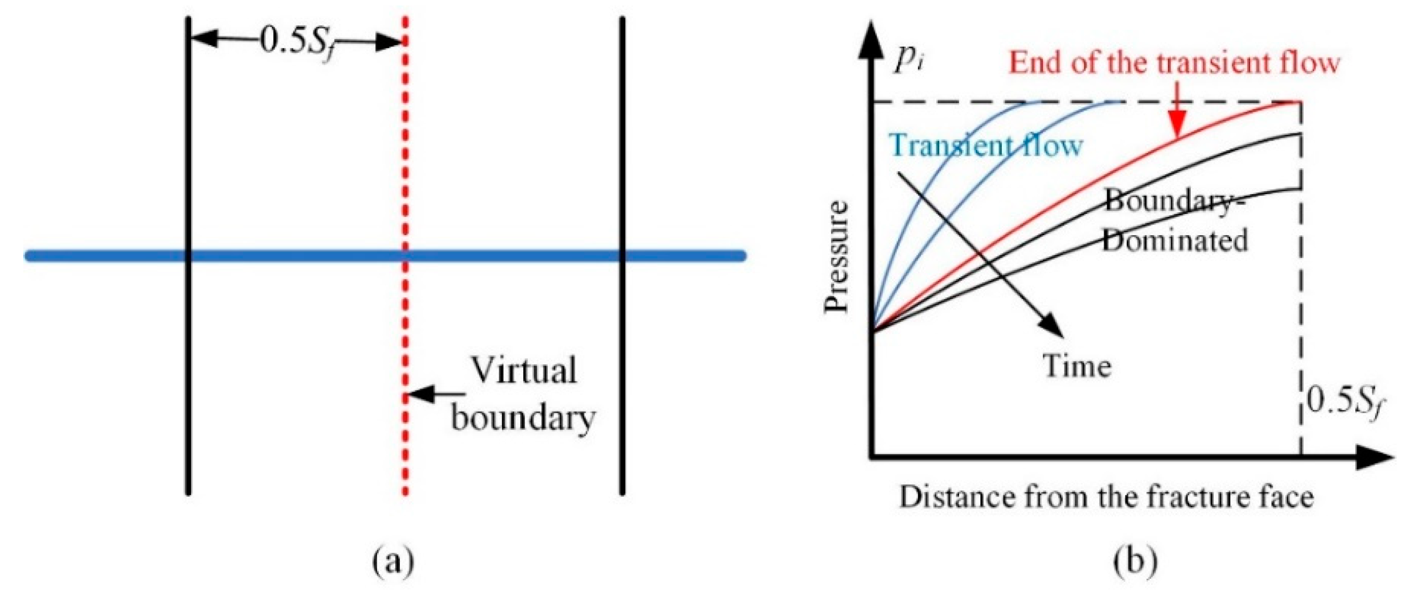
Four flow regimes may exist in multi-fractured reservoirs: (1) early time reservoir linear flow (transient flow), (2) mid-time boundary-dominated flow, (3) late time reservoir radial flow, and (4) very late time bounded flow. For wells in shale plays the third and fourth flow regimes usually are not seen due to the ultralow permeability of shale matrix. To fully understand the performance of multi-fractured horizontal wells, we identify the first two flow regimes between fractures. Figure 1a presents two fractures with an assumption of a virtual boundary between these two fractures. In the transient flow period, pressure propagates outward from the fracture face without encountering the virtual boundary. In the boundary-dominated flow period, the pressure transient has reached the virtual boundary, and the static pressure is declining at the boundary, as shown in Figure 1b.
In this section, the log-log diagnostic plots of production rate versus real production time as well as material balance time (MBT) are constructed to identify the flow regime of TMS wells. The procedure for identifying the flow regime is as follows [30].
Construct the production rate versus real production time curve (i.e., PT curve) and production rate versus material balance curve (i.e., MBT curve) on the same log-log plot. Then plot a tangent line LMBT using the end of MBT curve. If the slope kMBT of the tangent line LMBT is close to −1, then we have confidence that the boundary-dominated flow regime has been reached. If the slope kMBT is greater than -1, one can move the line LMBT onto the PT curve and get an approximately tangent point P. We draw another tangent line LPT using data between point P and the end of production data. If the slope kPT of this line is less than or equal to −1, it is believed that the well has reached the boundary-dominated regime, and the real production time corresponding to point P is the estimated switching time from transient flow to the boundary-dominated flow. However, if it is difficult to draw a tangent line LPT with slope kPT less than or equal to −1 owing to few points after point P, then one failed to obtain the conclusion that the well has reached boundary-dominated flow.
3.2. TMS Well Description
The study area in Mississippi is presented in Figure 2. The shapes for Louisiana and Mississippi counties were downloaded from the website (https://www2.census.gov). The production data as of May 2018 were gathered from 55 TMS wells in Mississippi from the Alfred C. Moore, Pearl River, and Henry Fields. These data were downloaded from the Mississippi Automated Resource Information System (MARIS) website (www.maris.state.ms.us).
Quality control of the production data was performed to validate the compliance of the field data with the assumptions used in the analysis. Those wells that had abrupt changes in monthly oil production rate during the production history were removed. This helps minimize the influence of changes in the production operations that would have a great effect on the production history. Following this, seven TMS wells that had reached the boundary-dominated flow regime were analyzed. Other wells could not be analyzed because of absence of a definite trend in the reported production data, most likely dictated by the used production strategy for which no details are available.
It should be stated that other wells may also have reached the boundary-dominated flow regime. However, we did not analyze these wells due to lack of completion data and also abrupt changes in production data of these wells over time. Seven TMS wells used in this study are shown as blue dots in Figure 2. The wells’ labels and their locations are listed in Table 1. Proppant has a major impact on fracture conductivity. Unfortunately, the type of proppant used in these seven TMS wells could not be identified due to the lack of completion data. The average fracture spacing can be estimated by using the stages.
3.3. Flow Regimes of TMS Wells
Figure 3 shows the log-log diagnostic plot of the seven TMS wells. Well 1 has a horizontal length of 9102 ft and an effective lateral length of 8442 ft with 29 stages, and each stage has four clusters. We drew a tangent line of MBT curve and found that the production data at the end of material balance time lies on the tangent line LMBT with a slope of −0.779. As kMBT is less than −1, the tangent line, LMBT, was moved onto the PT curve, and it showed tangency to this curve. If we draw a tangent line LPT using production data vs. real production time. The slope kPT is found to be −1.085, indicating a typical behavior of boundary-dominated flow over 16 months of production.
Well 2 was drilled and completed with an effective lateral length of 6757 ft and a 22 stage hydraulic fracturing operation. We can see from Figure 3b that the slopes of MBT curve (kMBT) and PT curve (kPT) are −0.688 and −1.002, respectively, indicating that well 2 should be in the boundary-dominated flow regime with an estimated switching time of 9.5 months.
Well 3 was drilled and completed with a 4,508 ft lateral and a ten stage hydraulic fracturing operation. From this plot, we can see that kMBT and kPT are −0.845 and −1.295, respectively. Therefore, we have confidence that well 3 switched from the transient flow to the boundary-dominated flow over 27 months of production. Figure 3c also shows that well 3 experienced a long-term transient flow for over two years.
Well 4 has a true vertical depth of 11,489 ft and an effective lateral length of 6451 ft with 26 stages. We can see from Figure 3d that well 4 has reached the boundary-dominated flow regime as the slope kPT is less than −1. The estimated switching time from the transient flow to the boundary-dominated flow is 12 months.
Well 5 has a true vertical depth of 12,245 ft and an effective lateral length of 5601 with 24 stages. It can be seen from Figure 3e that the diagnostic plot that the slope kMBT and kPT are −0.733 and −1.123, indicating a boundary-dominated flow regime.
Well 6 has a true vertical depth of 12,016 ft and an effective lateral length of 6,681 ft with 25 stages. From the diagnostic plot Figure 3f, we can see that kMBT and kPT are −0.787 and −1.173, indicating it reached the boundary-dominated flow regime in over 13 months of production.
The true vertical depth and effective lateral length of well 7 are 11,841 and 5681 ft, respectively. Slope kMBT and kPT are found to be −0.714 and −0.988, respectively. As kPT is approximately close to −1, well 7 should be in the boundary-dominated flow regime in over 13 months from its first production month.
4. Model Verification
4.1. Verification of the Model on Simulated Production Dataset
To verify the proposed model, we compared the model-predicted production rates with simulation results calculated by COMSOL Multiphysics. Figure 4 shows the grid of the model. Fluid flow in the half fracture (xf) and half spacing (0.5Sf) area is modeled for convenience. In this case, Darcy’s law in the subsurface flow module was used to model fluid flow within the porous medium. The hydraulic fracture was represented by a boundary layer with a thickness of 0.5 w (i.e., line AB). The decline of fracture conductivity is modeled using equation (A3). The following assumptions were made in this section: the fracture half-length was 300 ft, the fracture spacing was 60 ft, the initial reservoir pressure was 6,200 psia, the bottom hole pressure was 4,000 psia (at point A), the fracture height was 100 ft, the matrix permeability was 0.0002 md, the number of clusters was 120, the porosity was 8%, the oil formation factor was 1.5 rb/stb, the oil viscosity was 0.5 cp. We compared six cases, case 1: Cf0 = 2 md-ft, and cp = 0.0005 psia−1; case 2: Cf0 = 2 md-ft, and cp = 0.001 psia−1; case 3: Cf0 = 5 md-ft, and cp = 0.0005 psia−1; case 4: Cf0 = 5 md-ft, and cp = 0.001 psia−1; case 5: Cf0 = 10 md-ft, and cp = 0.0005 psia−1; case 6: Cf0 = 10 md-ft, and cp = 0.001 psia−1.
If the predicted production rates match the simulation results, the variation of fracture conductivity can be captured using the proposed analytical model based on the production data under boundary-dominated flow conditions. R-square (R2) and average absolute relative error percentage (AAREP) were utilized to estimate the proposed model. AAREP is defined as [31,32],
where N is the number of data points; Oi is the observed data; Ei is the predicted data.
The fracture compressibility can be obtained by fitting the proposed model to the production rate calculated by COMSOL. Figure 5 compares the oil production rate calculated by the proposed model and that of COMSOL Multiphysics software. After 40 months of production, the fracture conductivity was reduced by 53% and 69% for case 1 and case 2, respectively. The comparison between the prescribed fracture conductivity and the predicted value is presented in Table 2. Besides, there is good agreement between the prescribed fracture compressibility and the model-predicted value, with relative differences of fracture compressibility of less than 10%.
4.2. Analysis of TMS Well Data
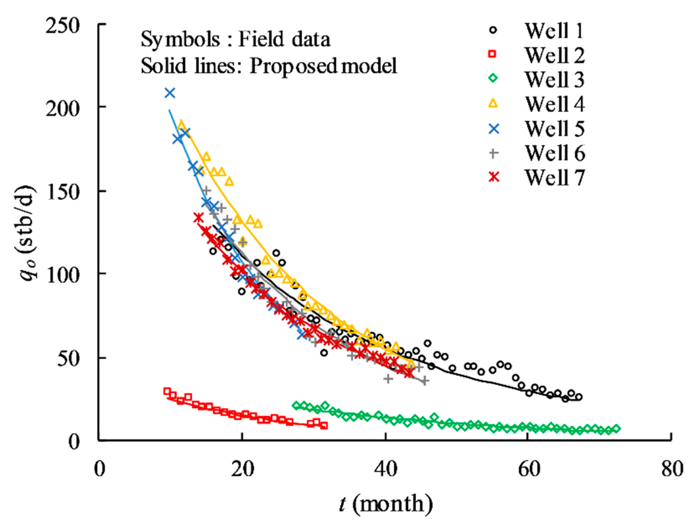
Figure 6 shows the comparison of field data and predicted values for the seven TMS wells studied in this paper. The calculated R2 and AAREP values are listed in Table 3. For example, well 1 produced 1072 barrels of oil equivalent per day during the first 30 days of production. Even though this well produced considerable amounts of hydrocarbons, its production rate decreased to 120 stb/d over 16 months of production. After 16 months, the cumulative oil production was 148,762 bbl. The R2 and AAREP are 0.925 and 10.38%, respectively. In general, relatively high R2 and low AAREP values were observed, indicating a good agreement between the field data and predicted results.
5. Variation of Fracture Conductivity
Figure 7 presents the variation of the predicted fracture conductivity with time for the seven TMS wells. The fitted fracture compressibility is listed in Table 3. The numerical method used to calculate the fracture conductivity is demonstrated in Appendix A. The fracture conductivity changes over time owing to depletion of pressure in the hydraulic fractures. Previous studies found that time-dependent fracture conductivity changes in logarithmic or exponential types [28]. It is evident from Figure 7 that the fracture conductivity for these TMS wells varies logarithmically with the production time. Take well 1 as an example. The fracture conductivity at the switching time is about 0.63 times its initial value, which gives an average decline rate of 27.3% per year in the transient flow period. The fracture conductivity was reduced by 52% over 65 months of production. We can see that the variation of fracture conductivity in the transient flow period is more significant than that in the boundary-dominated flow period.
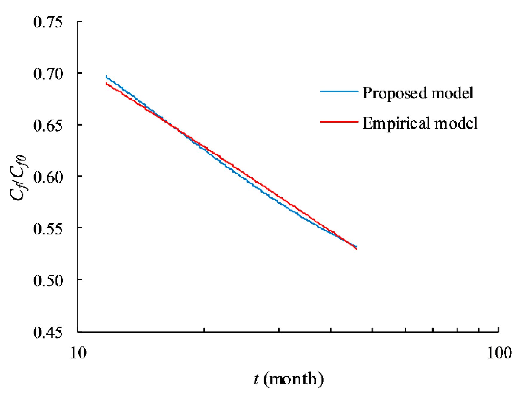
We also compared the time-dependent fracture conductivity with the empirical model expressed by [28],
where t is the production time in months, χ is the dimensionless coefficient describing the time-dependent fracture conductivity.
Figure 8 shows the comparison of fracture conductivity of well 4 between our proposed model and the empirical equation. A summary of R2 and AAREP values for the seven TMS wells is listed in Table 4. From Figure 8 we can see that the empirical equation exhibits a linear trend on the semi-log plot. Our proposed model predicts an S-type decline curve. The dimensionless coefficient χ has been found in the range of 0.116~0.130 with an average of 0.123 for the seven wells. Very high values of R2 and extremely low AAREP values have been observed, indicating excellent goodness of fit between our proposed model and the empirical equation.
6. Discussion
A mathematical model was developed in this study to capture the pressure-dependent decline of fracture conductivity from production data. As stated previously, the newly proposed model is suitable for wells with production in the boundary-dominated flow period. It has been recognized that the production rate declines with material balance time with slopes of −1/2 and −1 during the linear flow and boundary-dominated flow periods, respectively, in the log-log plot when there is no skin effect [33]. Many multi-fractured horizontal wells producing from shale reservoirs have been reported to experience a long-term linear flow (transient flow) period. The presence of decline of fracture conductivity and formation damage is usually interpreted as skin factor, which may change the shape of the diagnostic plot [22]. Nobakht and Mattar [34] stated that the linear flow is no longer a straight line with a slope of −1/2 other than the late-time data. They suggested using the square-root-of-time plot to identify the linear flow. Sun et al. [28] investigated the influence of time-dependent fracture conductivity on the production decline curves. Their study indicated that both formation damage and time-dependent fracture conductivity could not delay the time that the reservoir entered the boundary-dominated flow. Their influences on production decline are mainly seen at the early stage. Therefore, the log-log diagnostic method proposed by Zhou et al. [30] was used to identify the boundary-dominated flow regime rather than the linear flow regime in the present study. The log-log diagnostic approach is an effective method to avoid misinterpretation and to estimate the switching point.
The switching time from the transient flow to the boundary-dominated flow can also be estimated using the concept of radius-of-investigation [35],
where telf is the switching time in hours, ϕ is the porosity, ct is the total compressibility in psia−1.
From Equation (7) we can see that the switching time is highly related to the fracture spacing and the matrix permeability. A decrease in fracture spacing will reduce the switching time, provided that the matrix permeability is held constant. As the matrix permeability decreases, the expected switching time increases. Therefore, the long-term transient flow period may be attributed to either the ultralow permeability of the TMS or large fracture spacing.
Besides, it is assumed that the matrix permeability is constant. Besov et al. [2] hold the opinion that the TMS is different from other shale reservoirs because its pores cannot store hydrocarbons. Their experiments showed that the porosity of TMS formation is contained within its inorganic pores. They also indicated that hydrocarbons are more likely to be stored and produced from microfractures of TMS. It is well known that the permeability of microfractures exhibits stress sensitivity, which may delay the switching time from the transient flow to the boundary-dominated flow [28]. To simulate the fluid transport capacity of fractures during the whole life of hydrocarbon production where formation pressure declines and thus effective stress increases, the variation of microfracture permeability values need to be predicted. Our future work will focus on the conductivity of natural fracture and its influence on the production decline behavior of TMS.
Another limitation in our current study is that the proposed model can only estimate the pressure-dependent decline of fracture conductivity in the boundary-dominated flow period. Equation (A3) was developed for fractures filled with different materials such as clay (relatively mechanically unstable) and silica (mechanically stable). In the present study, we modified this equation to predict the conductivity of propped fractures. It is understood that hydraulic fracture conductivity is highly related to the closure stress, formation hardness, and proppant properties, etc. Once pumping is stopped, the fracture conductivity diminishes owing to proppant pack compaction and embedment of proppant particles during the production stage [22]. This means the compressibility of the proppant pack defined in equation (4) may change with production. In this case, the following equation can be used to describe the variation of the compressibility of the proppant pack [36],
where α is the decline rate of the propped fracture compressibility with increased effective stress, cp0 is the initial compressibility of the proppant pack, σe is the effective stress, σe0 is the initial effective stress.
As we stated in Appendix A, the propped fracture compressibility is assumed to be constant to simplify the solution. Results observed from the current study will be checked and further improved.
7. Conclusions
An analytical model was developed for capturing the pressure-dependent decline of fracture conductivity in the TMS fields from production data. The following conclusions are drawn:
- (1)
- The log-log diagnostic approach was used to identify the boundary-dominated flow regime of seven TMS wells. The results indicated that these seven wells exhibited a long-term transient flow period.
- (2)
- The R-square and AAREP were utilized in this study to estimate the performance of the proposed analytical well productivity model considering time-dependent fracture conductivity. The results indicated that the proposed model allows approximation of the real production data of the project wells in TMS formation with good accuracy.
- (3)
- The proposed fracture conductivity model was verified against simulated production data for a wide range of fracture conductivities/compressibilities. The results indicated that the predicted fracture compressibilities agree well with the prescribed values, with relative differences of fracture compressibility that were less than 10%.
- (4)
- The revealed average fracture conductivity decreases over time in the range of 100%-48% of the initial fracture conductivity. The pressure-dependent decline of fracture conductivity can be approximated using a logarithmic function given by equation (6) with the dimensionless coefficient χ varying between 0.116 and 0.130.
Author Contributions
Investigation, X.Z.; Methodology, X.Y.; Resources, B.G.; Supervision, B.G.; Validation, X.Z.; Writing – original draft, X.Y.
Funding
This research was supported by the U.S. DOE project (Project No. DE-FE0031575).
Conflicts of Interest
The authors declare no conflict of interest.
Nomenclature
| A | constant defined by Equation (1) |
| AAREP | average absolute relative error percentage |
| Bo | oil formation factor, rb/stb |
| c | defined by Equation (1) |
| c1 | defined by Equation (A12) |
| c2 | defined by Equation (A14) |
| Cf | fracture conductivity, md-ft |
| Cf0 | initial fracture conductivity, md-ft |
| cp | compressibility of the proppant pack, psia−1 |
| cp0 | initial compressibility of the proppant pack, psia−1 |
| ct | total reservoir compressibility, psia−1 |
| Ei | model-predicted production rate, stb/d |
| h | fracture height, ft |
| kf | fracture permeability, md |
| kf0 | initial fracture permeability, md |
| km | matrix permeability, md |
| N | number of production data points |
| nf | number of hydraulic fractures |
| Ni | initial oil in place in the drainage area of the well, stb |
| Np | cumulative oil production from the well, stb |
| Np1 | cumulative oil production at point 1, stb |
| Np2 | cumulative oil production at point 2, stb |
| Oi | observed production rate, stb/d |
| pi | initial reservoir pressure, psia |
| average formation pressure, psia | |
| pw | wellbore pressure, psia |
| qo | oil production rate, stb/d |
| qo1 | oil production rate at point 1, stb/d |
| qo2 | oil production rate at point 2, stb/d |
| Sf | fracture spacing, ft |
| telf | time at the end of transient flow, hour |
| w | fracture width, inch |
| xf | fracture half-length, ft |
| αb | Biot coefficient |
| μo | oil viscosity, cp |
| σe | effective stress, psi |
| σe0 | initial effective stress, psi |
| ϕ | matrix porosity |
| α | decline rate of the propped fracture compressibility, psia−1 |
| ν | Poison’s ratio |
Appendix A. Derivation of Productivity Model with Pressure-Dependent Fracture Conductivity
This section provides the derivation of an analytical model to capture the pressure-dependent decline of fracture conductivity from production data. Li et al. [35] proposed an analytical model for predicting the productivity of multi-fractured shale oil wells. The following assumptions are made,
- The oil formation is isotropic.
- Boundary-dominated flow has been reached within the fracture drainage area.
- Linear flow prevails from the shale matrix to the fractures.
- Fracture and formation damages are negligible.
- No change in fluid composition during production.
- Hydraulic fractures have the same geometry.
- Reservoir pressure is above the bubble point pressure.
As stated by Li et al. [35], it is not always valid to make the sixth assumption. However, it is acceptable for developing a simple analytical model. The oil production rate is [35],
where
where is the average formation pressure, kf is hydraulic fracture permeability, and w is the average fracture width.
It is generally believed that fracture conductivity plays an essential role in well performance. In the present study, we take the pressure-dependent decline of fracture into account. Chen et al. [36] developed a model to predict the conductivity of fractures filled with some porous materials such as carbonate and silica. It is assumed that the fracture conductivity of the propped fracture (kf∙w) can also be described by the following equation [36],
To simplify the model, it is assumed that the compressibility of the proppant pack is constant [37]. Substituting Equation (A3) into Equation (A2) gives,
Under the condition that reservoir pressure is above the bubble point pressure, based on the material balance equation,
The average reservoir pressure is expressed as,
Substituting Equation (A6) into Equations (A1) and (A4) yields,
Equation (A7) is simplified as,
where
To determine the values of cp in Equation (A8) and A in Equation (A9) using production data, select two points in the trend where,
where
and
where
Solving Equations (A11) and (A13), one can get the values of cp and A. Then the variation of fracture conductivity during production can be determined by substituting Equation (A6) into Equation (A3),
If desired, Equation (A9) can be used for predicting future production. The procedure is outlined as follows,
- Tabulate a column of qo values from the present oil production rate to the abandonment oil production rate.
- Use a numerical algorithm to solve Equation (A9) for a column of Np values.
- Construct columns of Np.
- Construct a column of t by dividing Np by qo.
- Construct a column of t based on t = ∑Δt.
- Plot qo versus t columns for a future production curve.
References
- Allen, J.E.; Meylan, M.A.; Heitmuller, F.T. Determining hydrocarbon distribution using resistivity, Tuscaloosa Marine Shale, southwestern Mississippi. Gulf Coast Assoc. Geol. Soc. Trans. 2014, 64, 41–57. [Google Scholar]
- Besov, A.; Tinni, A.; Sondergeld, C.; Rai, C.; Paul, W.; Ebnother, D.; Smagala, T. Application of laboratory and field NMR to characterize the Tuscaloosa Marine Shale. Petrophysics 2017, 58, 221–231. [Google Scholar]
- Berch, H.; Jeffrey, N. Predicting potential unconventional production in the Tuscaloosa Marine Shale play using thermal modeling and log overlay analysis. GCAGS J. 2014, 3, 69–78. [Google Scholar]
- John, C.J.; Jones, B.L.; Moncrief, J.E.; Bourgeois, R.; Harder, B.J. An unproven unconventional seven billion barrel oil resource-the Tuscaloosa Marine Shale. LSU Basin Res. Inst. Bull. 1997, 7, 1–22. [Google Scholar]
- Stewart, G. Integrated analysis of shale gas well production data. In Proceedings of the SPE Asia Pacific Oil & Gas Conference and Exhibition, Adelaide, Australia, 14–16 October 2014. [Google Scholar]
- Yang, C.; Sharma, V.K.; Detta-Gupta, A.; King, M.J. A novel approach for production transient analysis of shale gas/oil reservoirs. In Proceedings of the Unconventional Resources Technology Conference, San Antonio, TX, USA, 20–22 July 2015. [Google Scholar]
- Bajwa, A.I.; Blunt, M.J. Early-time 1D analysis of shale-oil and -gas flow. SPE J. 2016, 21, 1254–1262. [Google Scholar] [CrossRef]
- Cheng, Y. Pressure transient characteristics of hydraulically fractured horizontal shale gas wells. In Proceedings of the SPE Eastern Regional Meeting, Columbus, OH, USA, 17–19 August 2011. [Google Scholar]
- Sun, H.; Dengen, Z.; Adwait, C.; Meilin, D. Quantifying shale oil production mechanisms by integrating a Delaware basin well data from fracturing to production. In Proceedings of the SPE/AAPG/SEG Unconventional Resources Technology Conference, San Antonio, TX, USA, 1–3 August 2016. [Google Scholar]
- Yu, W.; Yu, Y.; Wu, K.; Sepehrnoori, K. Impact of well interference on shale oil production performance: A numerical model for analyzing pressure response of fracture hits with complex geometries. In Proceedings of the SPE Hydraulic Fracturing Technology Conference and Exhibition, Woodlands, TX, USA, 24–26 January 2017. [Google Scholar]
- Ali, T.A.; Sheng, J.J. Production decline models: A comparison study. In Proceedings of the SPE Eastern Regional Meeting, Morgantown, WV, USA, 13–15 October 2015. [Google Scholar]
- Duong, A.N. An unconventional rate decline approach for tight and fracture-dominated gas wells. In Proceedings of the Canadian Unconventional Resources and International Petroleum Conference, Calgary, AB, Canada, 19–21 October 2010. [Google Scholar]
- Vanorsdale, C.R. Production decline analysis lessons from classic shale gas wells. In Proceedings of the SPE Annual Technical Conference and Exhibition, New Orleans, LA, USA, 30 September–2 October 2013. [Google Scholar]
- Mattar, L.; Moghadam, S. Modified power law exponential decline for tight gas. In Proceedings of the Canadian International Petroleum Conference, Calgary, AB, Canada, 16–18 June 2009. [Google Scholar]
- Ali, T.; Sheng, J.; Soliman, M. New production-decline models for fractured tight and shale reservoirs. In Proceedings of the SPE Western North American and Rocky Mountain Joint Meeting, Denver, CO, USA, 17–18 April 2014. [Google Scholar]
- Kenomore, M.; Hassan, M.; Malakooti, R.; Dhakal, H.; Shah, A. Shale gas production decline trend over time in the Barnett Shale. J. Pet. Sci. Eng. 2018, 165, 691–710. [Google Scholar] [CrossRef]
- Clarkson, C.R. Production data analysis of unconventional gas wells: Workflow. Int. J. Coal Geol. 2013, 109, 147–157. [Google Scholar] [CrossRef]
- Xu, B.; Haghighi, M.; Li, X.; Cooke, D. Development of new type curves for production analysis in naturally fractured shale gas/tight gas reservoirs. J. Pet. Sci. Eng. 2013, 105, 107–115. [Google Scholar] [CrossRef]
- Shin, H.J.; Lim, J.S.; Shin, S.H. Estimated ultimate recovery prediction using oil and gas production decline curve analysis and cash flow analysis for resource play. Geosyst. Eng. 2014, 7, 78–87. [Google Scholar] [CrossRef]
- Ai, K.; Duan, L.; Gao, H.; Jia, G. Hydraulic fracturing treatment optimization for low permeability reservoirs based on unified fracture design. Energies 2018, 11, 1720. [Google Scholar] [CrossRef]
- Zhou, L.; Chen, J.; Gou, Y.; Feng, W. Numerical investigation of the time-dependent and the proppant dominated stress shadow effects in a transverse multiple fracture system and optimization. Energies 2017, 10, 83. [Google Scholar] [CrossRef]
- Wang, J.; Elsworth, D.; Ma, T. Conductivity evolution of proppant-filled hydraulic fractures. In Proceedings of the 52nd U.S. Rock Mechanics/Geomechanics Symposium, Seattle, WA, USA, 17–20 June 2018. [Google Scholar]
- Awoleke, O.O.; Zhu, D.; Hill, A.D. New propped-fracture-conductivity models for tight gas sands. SPE J. 2016, 21, 1508–1517. [Google Scholar] [CrossRef]
- Chang, X.; Guo, Y.; Zhou, J.; Song, X.; Yang, C. Numerical and experimental investigations of the interactions between hydraulic and natural fractures in shale formations. Energies 2018, 11, 2541. [Google Scholar] [CrossRef]
- Zhang, J.; Ouyang, L.; Zhu, D.; Hill, A.D. Experimental and numerical studies of reduced fracture conductivity due to proppant embedment in the shale reservoir. J. Pet. Sci. Eng. 2015, 130, 37–45. [Google Scholar] [CrossRef] [Green Version]
- Teng, W.; Qiao, X.; Teng, L.; Jiang, R.; He, J. Production performance analysis of multiple fractured horizontal wells with finite-conductivity fractures in shale gas reservoirs. J. Nat. Gas Sci. Eng. 2016, 36, 747–759. [Google Scholar] [CrossRef]
- Wen, Q.; Zhang, S.; Wang, L. Influence of proppant embedment on fracture long term flow conductivity. Nat. Gas Ind. 2005, 25, 65–68. [Google Scholar]
- Sun, H.; Ouyang, W.; Zhang, M.; Tang, H.; Chen, C.; Xu, M.A. Advanced production decline analysis of tight gas wells with variable fracture conductivity. Pet. Explor. Dev. 2018, 45, 472–480. [Google Scholar] [CrossRef]
- Marsden, J.; Kostyleva, I.; Fassihi, M.R.; Gringarten, A.C. A conceptual shale gas model validated by pressure and rate data from the Haynesville Shale. In Proceedings of the SPE Annual Technical Conference and Exhibition, San Antonio, TX, USA, 9–11 October 2017. [Google Scholar]
- Zhou, P.; Pan, Y.; Sang, H.; Lee, W.J. Criteria for proper production decline models and algorithm for decline curve parameter inference. In Proceedings of the SPE/AAPG/SEG Unconventional Resources Technology Conference, Houston, TX, USA, 23–25 July 2018. [Google Scholar]
- Shi, X.; Yang, X.; Meng, Y.; Li, G. An anisotropic strength model for layered rocks considering planes of weakness. Rock Mech. Rock Eng. 2016, 49, 3783–3792. [Google Scholar] [CrossRef]
- Singh, M.; Samadhiya, N.K.; Kumar, A.; Kumar, V.; Singh, B. A nonlinear criterion for triaxial strength of inherently anisotropic rocks. Rock Mech. Rock Eng. 2015, 48, 1387–1405. [Google Scholar] [CrossRef]
- Rincones, M.D.; Lee, W.J.; Rutledge, J.M. Production forecasting for shale oil: Workflow. In Proceedings of the SPE Asia Pacific Unconventional Resources Conference and Exhibition, Brisbane, Australia, 9–11 November 2015. [Google Scholar]
- Nobakht, M.; Mattar, L. Analyzing production data from unconventional gas reservoirs with linear flow and apparent skin. J. Can. Pet. Technol. 2012, 51, 52–59. [Google Scholar] [CrossRef]
- Li, G.; Guo, B.; Li, J.; Wang, M. A mathematical model for predicting long-term productivity of modern multifractured shale gas/oil wells. SPE Drill. Completion 2019, 34. [Google Scholar] [CrossRef]
- Chen, D.; Pan, Z.; Ye, Z. Dependence of gas shale fracture permeability on effective stress and reservoir pressure: Model match and insights. Fuel 2015, 139, 383–392. [Google Scholar] [CrossRef]
- Neto, L.B.; Khanna, A.; Kotousov, A. Conductivity and performance of hydraulic fractures partially filled with compressible proppant packs. Int. J. Rock Mech. Min. Sci. 2015, 74, 1–9. [Google Scholar] [CrossRef]
Figure 1.
Schematic chart between two fractures. (a) Virtual boundary between two fractures. (b) Schematic chart of pressure distribution.
Figure 1.
Schematic chart between two fractures. (a) Virtual boundary between two fractures. (b) Schematic chart of pressure distribution.

Figure 2.
Map of the study area in Mississippi.
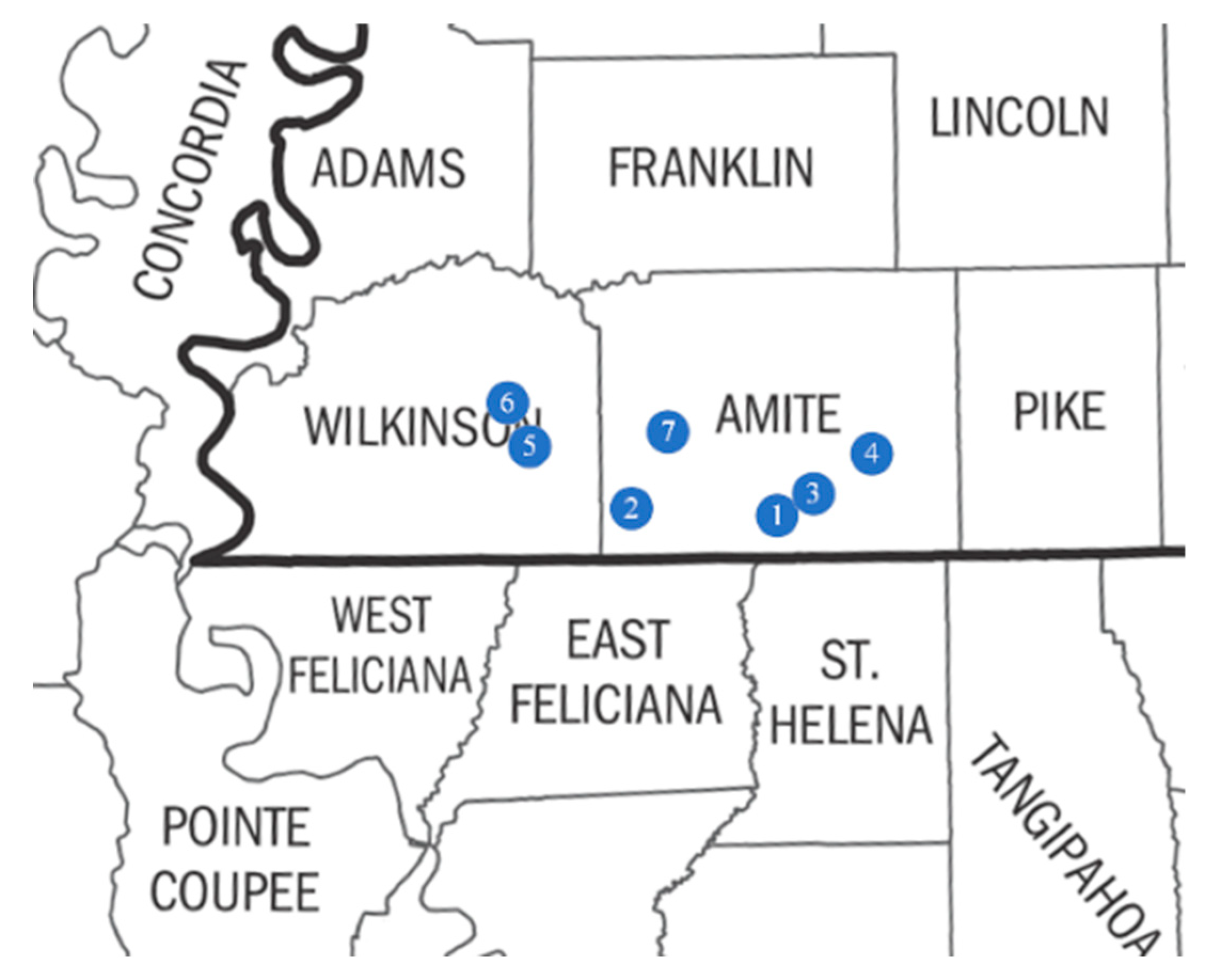
Figure 3.
Log-log diagnostic plot of TMS wells. (a) well 1. (b) well 2. (c) well 3. (d) well 4. (e) well 5. (f) well 6. (g) well 7.
Figure 3.
Log-log diagnostic plot of TMS wells. (a) well 1. (b) well 2. (c) well 3. (d) well 4. (e) well 5. (f) well 6. (g) well 7.

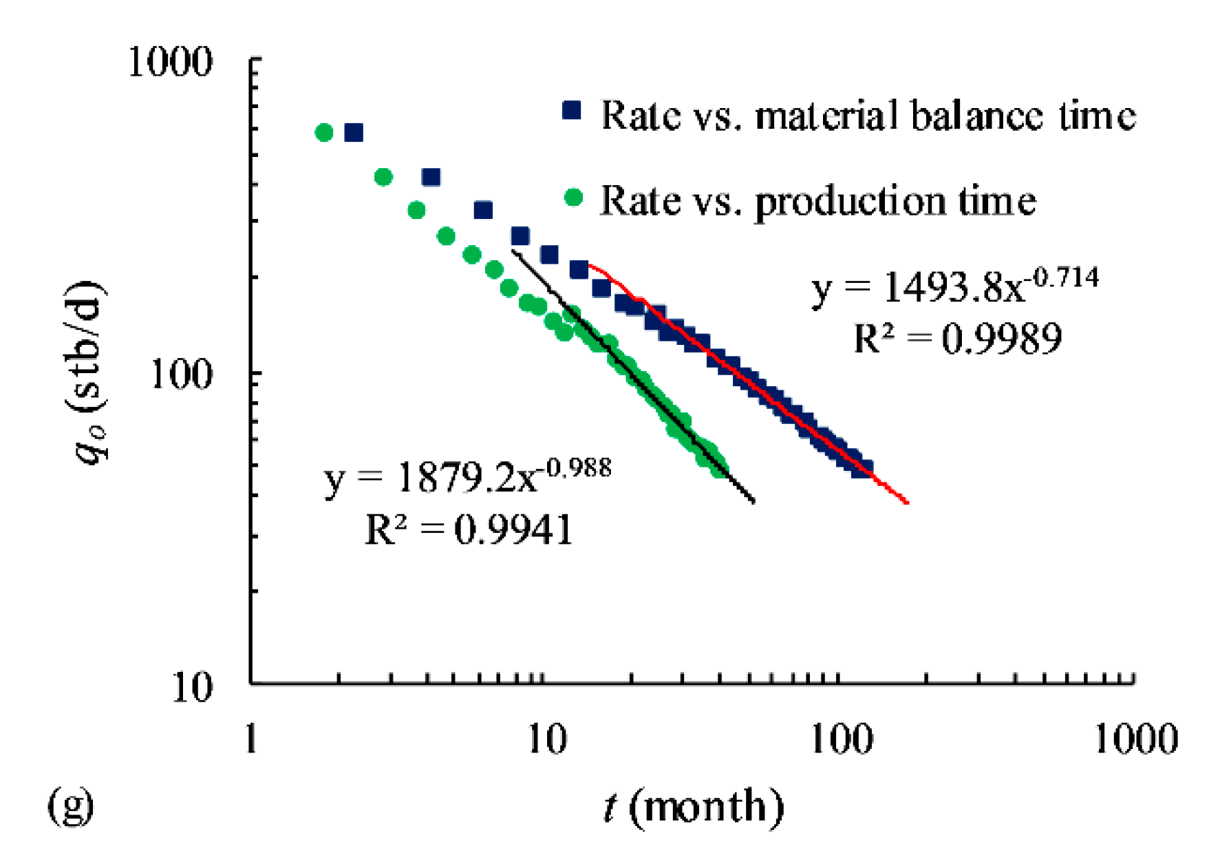
Figure 4.
Schematic diagram of grid structure of numerical model.

Figure 5.
Comparison between the model-predicted production rate and the simulation result.
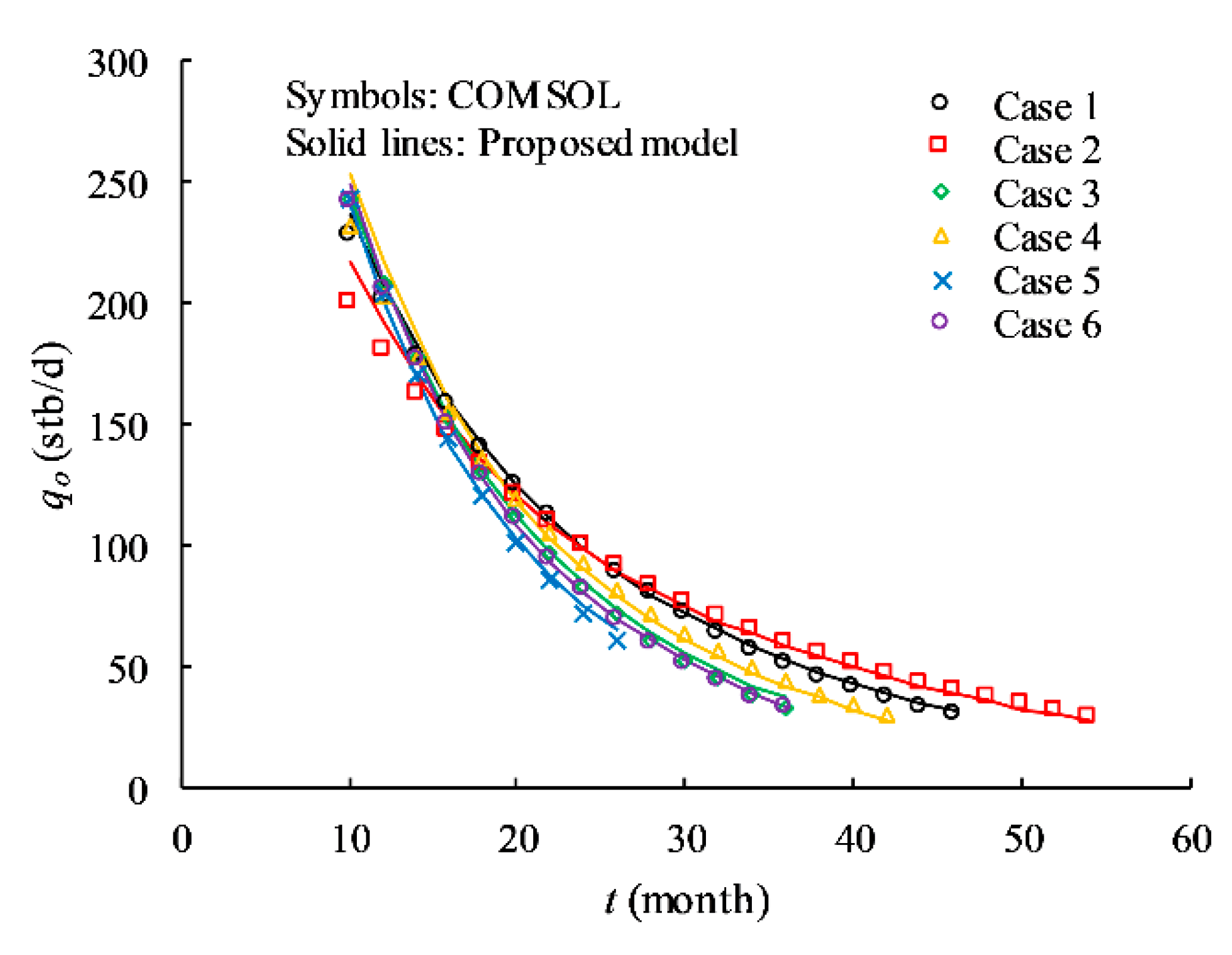
Figure 6.
Comparison of predicted and field data of TMS wells.

Figure 7.
Variation of fracture conductivity with production time for different wells.
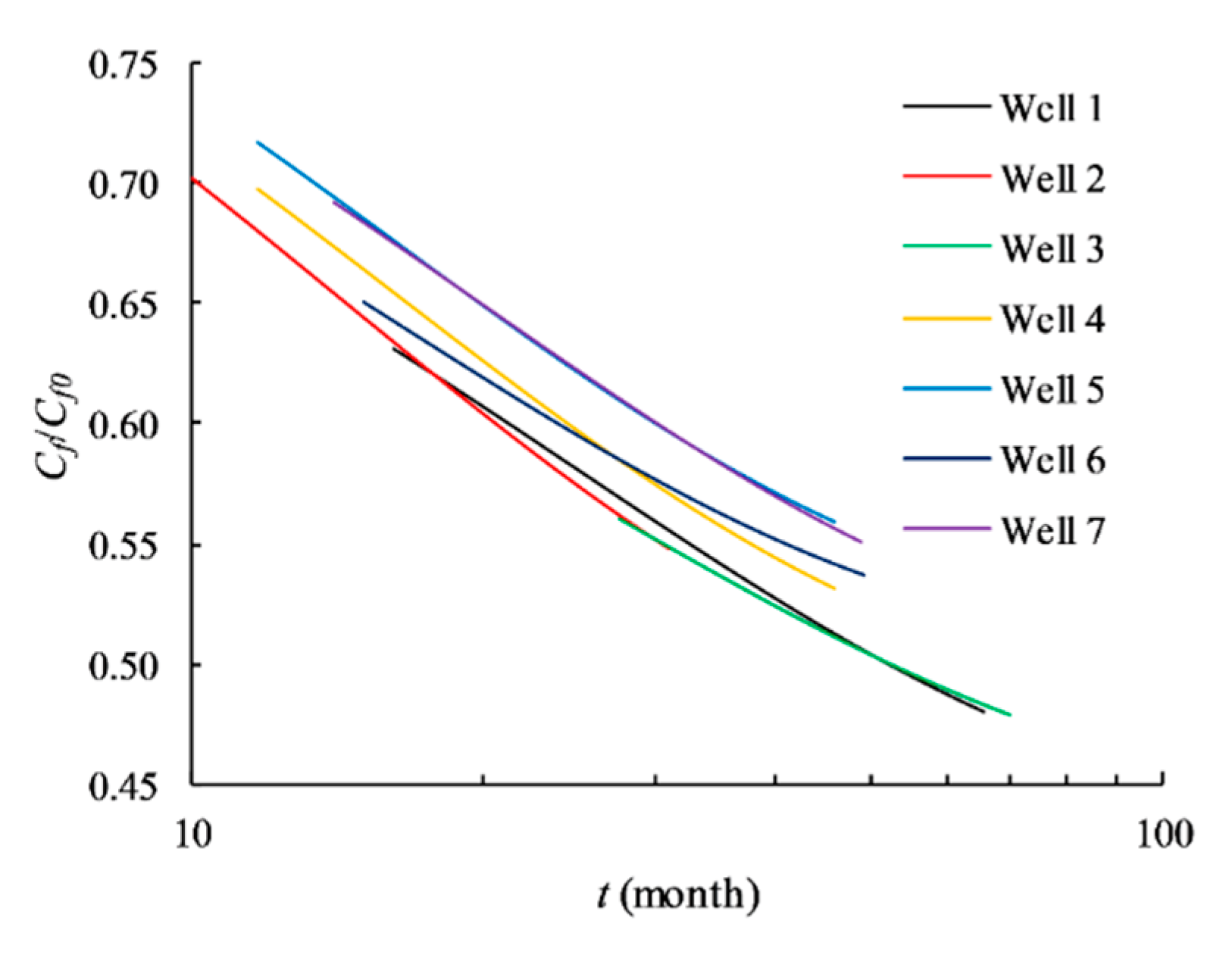
Figure 8.
Comparison of fracture conductivity of well 4 between the proposed model and the empirical model.
Figure 8.
Comparison of fracture conductivity of well 4 between the proposed model and the empirical model.

Table 1.
TMS wells used in this study.
| Well Label | True Vertical Depth (ft) | Effective Lateral Length (ft) | Frac Stages |
|---|---|---|---|
| 1 | 11,783 | 8442 | 29 |
| 2 | 12,598 | 6757 | 22 |
| 3 | 11,992 | 2923 | 10 |
| 4 | 11,489 | 6451 | 26 |
| 5 | 12,245 | 5601 | 24 |
| 6 | 12,016 | 6681 | 24 |
| 7 | 11,841 | 5681 | 25 |
Table 2.
Comparison between prescribed fracture conductivity and model-predicted value.
| No. | Oil Production rate (stb/d) | Fracture Compressibility (psia−1) | ||
|---|---|---|---|---|
| R2 | AAREP | COMSOL | Proposed Model | |
| Case 1 | 0.999 | 1.40% | 0.0005 | 0.00055 |
| Case 2 | 0.998 | 3.29% | 0.0010 | 0.00092 |
| Case 3 | 1.000 | 2.83% | 0.0005 | 0.00054 |
| Case 4 | 0.998 | 4.77% | 0.0010 | 0.00094 |
| Case 5 | 1.000 | 2.59% | 0.0005 | 0.00058 |
| Case 6 | 0.999 | 1.53% | 0.0010 | 0.00094 |
Table 3.
Calculated R2 and AAREP values for TMS wells.
| Well Label | Fracture Compressibility (psia−1) | R2 | AAREP |
|---|---|---|---|
| 1 | 0.00052 | 0.925 | 10.38% |
| 2 | 0.00056 | 0.960 | 5.71% |
| 3 | 0.00053 | 0.937 | 8.97% |
| 4 | 0.00047 | 0.978 | 4.65% |
| 5 | 0.00048 | 0.990 | 3.09% |
| 6 | 0.00052 | 0.974 | 6.27% |
| 7 | 0.00049 | 0.988 | 3.76% |
Table 4.
Calculated R2 and AAREP values for TMS wells.
| Well Label | χ | R2 | AAREP |
|---|---|---|---|
| 1 | 0.127 | 0.998 | 0.86% |
| 2 | 0.130 | 0.999 | 0.71% |
| 3 | 0.127 | 0.997 | 1.51% |
| 4 | 0.122 | 0.997 | 0.60% |
| 5 | 0.116 | 0.997 | 0.50% |
| 6 | 0.123 | 0.995 | 1.07% |
| 7 | 0.116 | 0.998 | 0.28% |
© 2019 by the authors. Licensee MDPI, Basel, Switzerland. This article is an open access article distributed under the terms and conditions of the Creative Commons Attribution (CC BY) license (http://creativecommons.org/licenses/by/4.0/).
Share and Cite
MDPI and ACS Style
Yang, X.; Guo, B.; Zhang, X. An Analytical Model for Capturing the Decline of Fracture Conductivity in the Tuscaloosa Marine Shale Trend from Production Data. Energies 2019, 12, 1938. https://doi.org/10.3390/en12101938
AMA Style
Yang X, Guo B, Zhang X. An Analytical Model for Capturing the Decline of Fracture Conductivity in the Tuscaloosa Marine Shale Trend from Production Data. Energies. 2019; 12(10):1938. https://doi.org/10.3390/en12101938
Chicago/Turabian StyleYang, Xu, Boyun Guo, and Xiaohui Zhang. 2019. "An Analytical Model for Capturing the Decline of Fracture Conductivity in the Tuscaloosa Marine Shale Trend from Production Data" Energies 12, no. 10: 1938. https://doi.org/10.3390/en12101938
Note that from the first issue of 2016, this journal uses article numbers instead of page numbers. See further details here.