A Large-Eddy Simulation-Based Assessment of the Risk of Wind Turbine Failures Due to Terrain-Induced Turbulence over a Wind Farm in Complex Terrain


1
Research Institute for Applied Mechanics (RIAM), Kyushu University, 6-1 Kasuga-kouen, Kasuga, Fukuoka 816-8580, Japan
2
Eurus Energy Holdings Corporation, 3-13, Toranomon 4-Chome, Minato-ku, Tokyo 105-0001, Japan
*
Author to whom correspondence should be addressed.
Energies 2019, 12(10), 1925; https://doi.org/10.3390/en12101925
Submission received: 3 April 2019
/
Revised: 10 May 2019
/
Accepted: 17 May 2019
/
Published: 20 May 2019
(This article belongs to the Special Issue Modeling of Wind Turbines and Wind Farms)
Abstract
:The first part of the present study investigated the relationship among the number of yaw gear and motor failures and turbulence intensity (TI) at all the wind turbines under investigation with the use of in situ data. The investigation revealed that wind turbine #7 (T7), which experienced a large number of failures, was affected by terrain-induced turbulence with TI that exceeded the TI presumed for the wind turbine design class to which T7 belongs. Subsequently, a computational fluid dynamics (CFD) simulation was performed to examine if the abovementioned observed wind flow characteristics could be successfully simulated. The CFD software package that was used in the present study was RIAM-COMPACT, which was developed by the first author of the present paper. RIAM-COMPACT is a nonlinear, unsteady wind prediction model that uses large-eddy simulation (LES) for the turbulence model. RIAM-COMPACT is capable of simulating flow collision, separation, and reattachment and also various unsteady turbulence–eddy phenomena that are caused by flow collision, separation, and reattachment. A close examination of computer animations of the streamwise (x) wind velocity revealed the following findings: As we predicted, wind flow that was separated from a micro-topographical feature (micro-scale terrain undulations) upstream of T7 generated large vortices. These vortices were shed downstream in a nearly periodic manner, which in turn generated terrain-induced turbulence, affecting T7 directly. Finally, the temporal change of the streamwise (x) wind velocity (a non-dimensional quantity) at the hub-height of T7 in the period from 600 to 800 in non-dimensional time was re-scaled in such a way that the average value of the streamwise (x) wind velocity for this period was 8.0 m/s, and the results of the analysis of the re-scaled data were discussed. With the re-scaled full-scale streamwise wind velocity (m/s) data (total number of data points: approximately 50,000; time interval: 0.3 s), the time-averaged streamwise (x) wind velocity and TI were evaluated using a common statistical processing procedure adopted for in situ data. Specifically, 10-min moving averaging (number of sample data points: 1932) was performed on the re-scaled data. Comparisons of the evaluated TI values to the TI values from the normal turbulence model in IEC61400-1 Ed.3 (2005) revealed the following: Although the evaluated TI values were not as large as those observed in situ, some of the evaluated TI values exceeded the values for turbulence class A, suggesting that the influence of terrain-induced turbulence on the wind turbine was well simulated.
1. Introduction
In recent years, wind power has started to be implemented across the world. In the midst of this movement, preparations for further dissemination of wind power are being advanced in Japan with the passage of the Act on Special Measures Concerning Procurement of Renewable Electric Energy by Operators of Electric Utilities. However, it is still true that there remain a large number of issues to be resolved for further dissemination of wind power. Some of these issues are technical, and they concern noise, lightning, and turbulence (terrain-induced turbulence). Terrain-induced turbulence is the main cause of the reduction of availability factors and wind turbine failures that increase repair costs, significantly affecting the wind power generation industry as a whole. Terrain-induced turbulence originates from the complexity of terrain. In Japan, where a larger proportion of the land is covered by mountains than in many countries abroad, areas for wind farm development are often characterized by complex terrain. Accordingly, the risk of wind turbine failure caused by terrain-induced turbulence is high in Japan. It should be noted that not all the wind turbines deployed on complex terrain break down because of terrain-induced turbulence. In addition, terrain undulations in complex terrain cause local increases of wind speed, which is considered to be an advantage. With the continuingly decreasing availability of flat areas for potential wind farm development, dissemination of wind power in Japan requires detailed business potential assessments, which involve highly accurate assessments of wind over complex terrain on local scales beforehand.
Deployment of a wind vane and an anemometer ensures the most reliable qualitative and quantitative confirmation of the presence of terrain-induced turbulence. However, over complex terrain, wind conditions can be different between two locations that are separated by several hundred meters; thus, the properties of terrain-induced turbulence assessed by a wind vane and an anemometer at a wind turbine site are not necessarily the same as those at another wind turbine site. From the perspective of cost, it is not feasible to deploy wind vanes and anemometers to all proposed wind turbine sites. In order to avoid unanticipated failures of wind turbines after wind farm construction, it is desirable to assess the risk of wind turbine failures, optimize the layout of the wind turbines, and select the most suitable wind turbine models prior to the construction of the wind farm.
Given the above background, the present study investigated the validity of a computational fluid dynamics (CFD)-based method for assessing the risk of wind turbine failures caused by terrain-induced turbulence at the planning stage of wind farm construction. CFD is a numerical simulation technique (software), which can simulate three-dimensional wind flow using computers [1,2,3,4,5,6,7,8,9,10,11,12]. The use of CFD software allows desktop assessment of wind flow for a potential wind farm prior to its actual construction. The Wind Atlas Analysis and Application Program (WAsP), developed by the Technical University of Denmark (DTU), is one such wind analysis software and has been commonly used in the wind power industry for some time [11,12]. However, because WAsP was developed for linear, steady flow analyses, its applicability for analyses of wind flow over complex terrain is highly limited. In recent years, nonlinear, unsteady flow analyses have become possible as a result of the rapid improvement of computers. A representative approach for such wind flow analyses uses a numerical turbulence model called large-eddy simulation (LES). In the present study, wind over an existing wind farm on complex terrain was analyzed with RIAM-COMPACT software, which was developed based on LES by the first author of the present paper [13,14,15,16,17,18,19,20,21]. At the wind farm investigated in the present study, failures of the yaw gears and motors that were likely caused by terrain-induced turbulence occurred frequently on only one particular wind turbine. Thus, the failure risk of the yaw gears and motors of this wind turbine was assessed by analyzing numerical simulation data.
2. An Overview of the Investigated Wind Farm, In Situ Data Analysis Results, and Discussions
Figure 1 shows a general view of the wind farm investigated in the present study. The wind farm and its surrounding area are characterized by highly complex terrain, and the wind turbines are deployed along a mountain ridge. At this wind farm, a total of 16 Siemens 1.3 MW, International Electrotechnical Commission (IEC) class IA wind turbines with a rotor diameter of 62 m and a hub height of 60 m have been deployed. The wind farm began operation in February 2004.
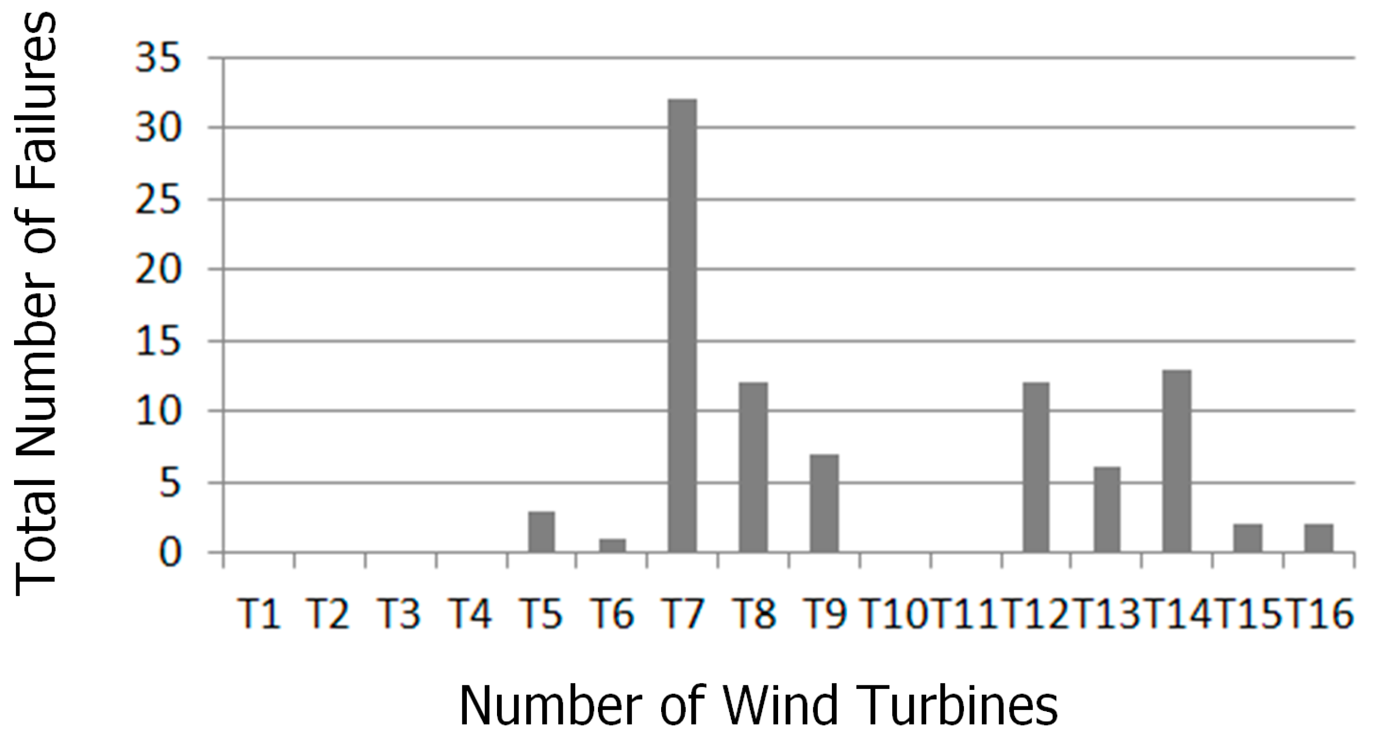
Figure 2 shows the total number of failures of the yaw gears and motors of each of the deployed turbines in the first seven years of the wind turbine operation. Figure 2 reveals that the number of failures at wind turbine #7 (T7) was larger by far than those at the other wind turbines.
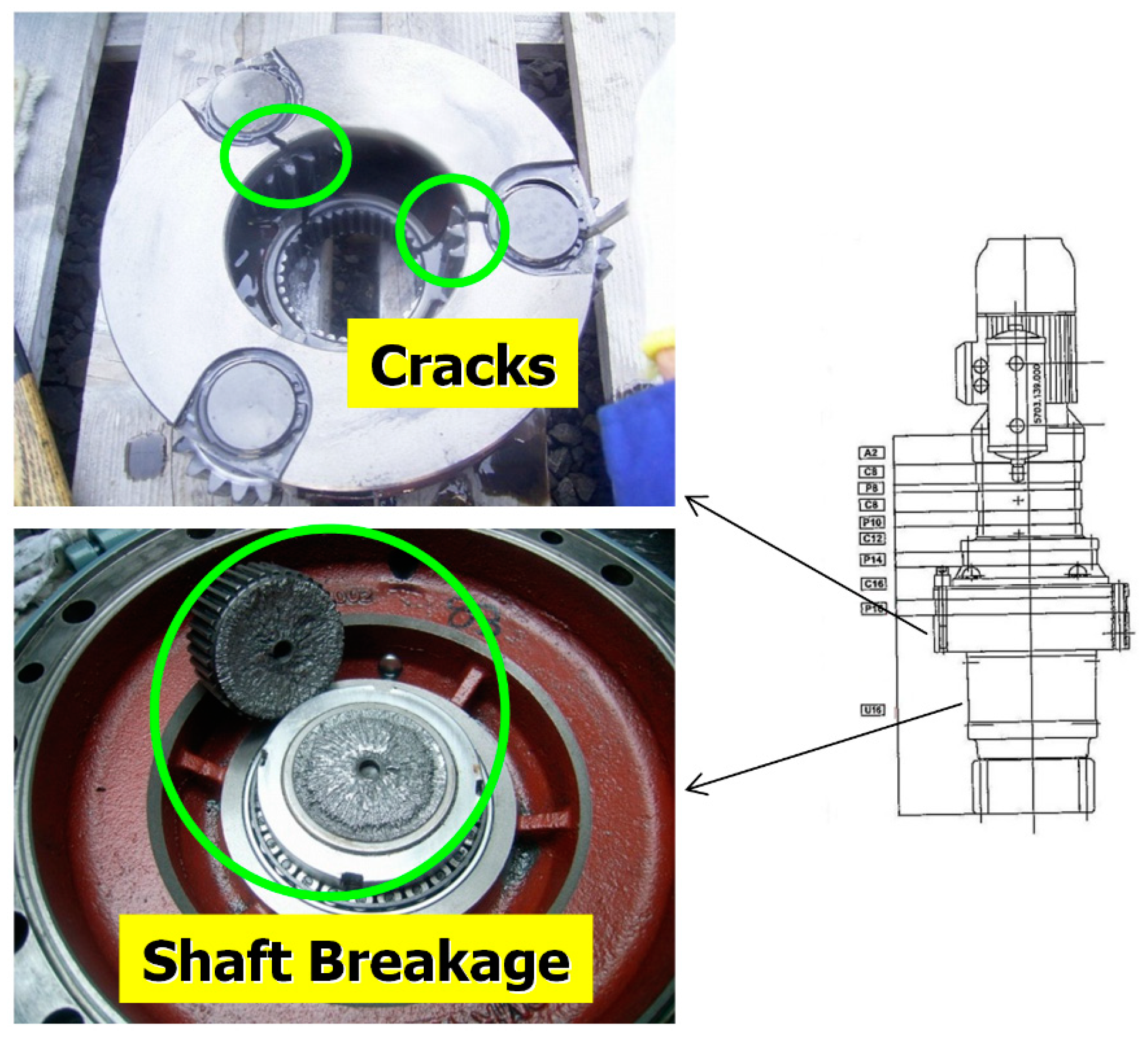
Figure 3 illustrates actual damage to a yaw gear. Cracks and shaft breakage can be identified, and it can be speculated that the damage occurred as a result of excessive force exerted on the yaw gear. Because the occurrence of cracks and shaft breakages was concentrated at T7, it was hypothesized that the cracks and shaft breakages at this turbine were attributable to a cause that was unique to this turbine. We presumed that a large number of the failures of T7 were caused by terrain-induced turbulence that originated from the terrain features in the area surrounding the wind turbine.
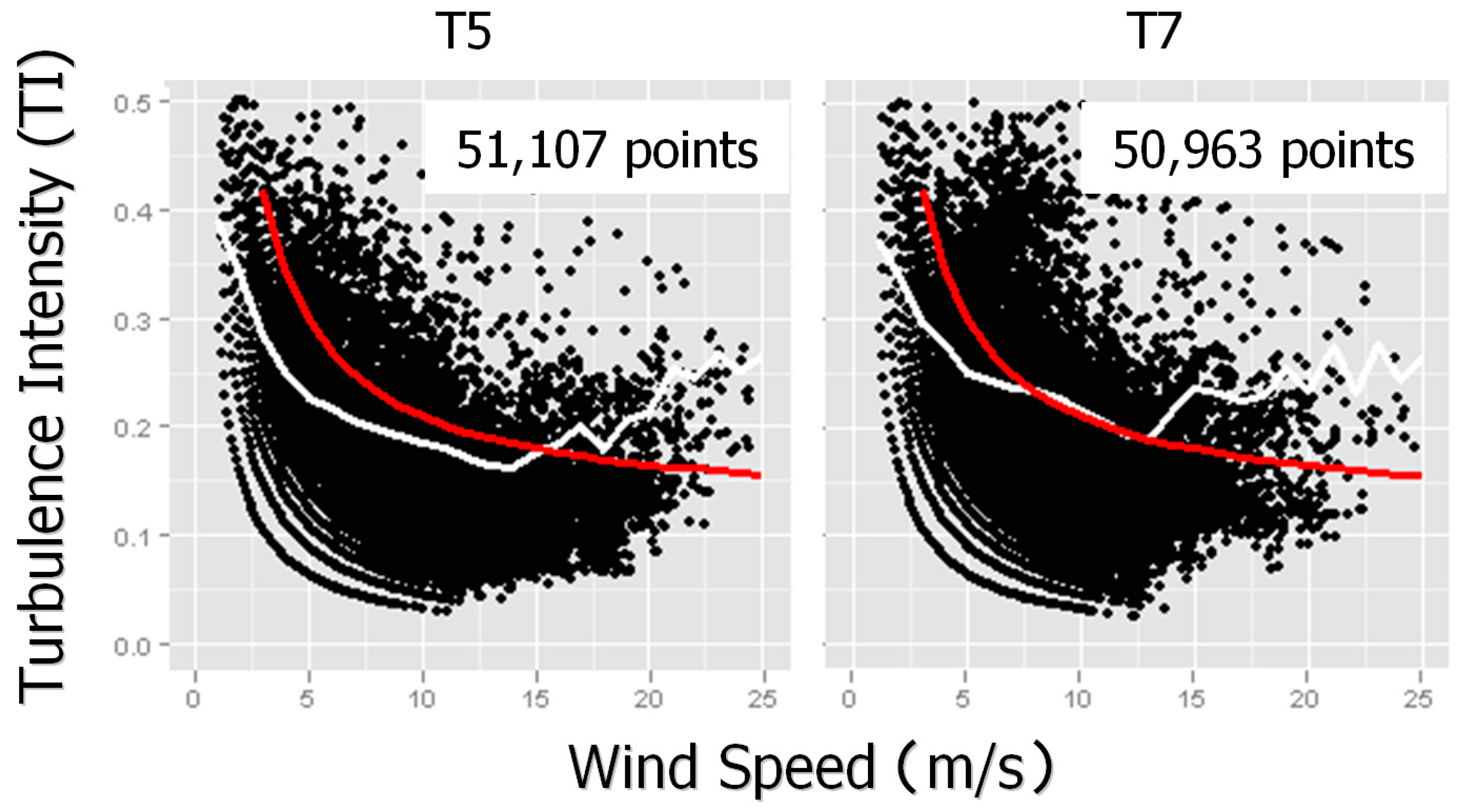
In order to examine the effect of terrain-induced turbulence on T7 in detail, the turbulence intensity (TI), evaluated from the Supervisory Control and Data Acquisition (SCADA) dataset for this wind turbine, was examined (Figure 4; see Equation (1) for the mathematical definition of TI). For comparison, Figure 4 also shows the TI evaluated from the SCADA dataset for wind turbine #5 (T5), which failed less often than T7. Each data point indicates a 10-min TI value. A close examination of Figure 4 reveals that the TI at T7 was slightly higher than that at T5. The red lines in Figure 4 show the relationship between TI and wind speed for turbulence class A (see Section 3.2 for details) from the Normal Turbulence Model (NTM) in 61400-1 Ed.3, IEC (2005). The white lines in Figure 4, which show the sum of the bin average and one bin standard deviation (σ) of the plotted TI values, indicate that the sum of these two values falls almost on the NTM line in the range of wind speeds greater than or equal to 7 m/s and less than 12 m/s for T7. For wind speeds of 12 m/s or higher, the sum of the two abovementioned values significantly exceeds the value of the TI for IEC turbulence class A from the NTM.
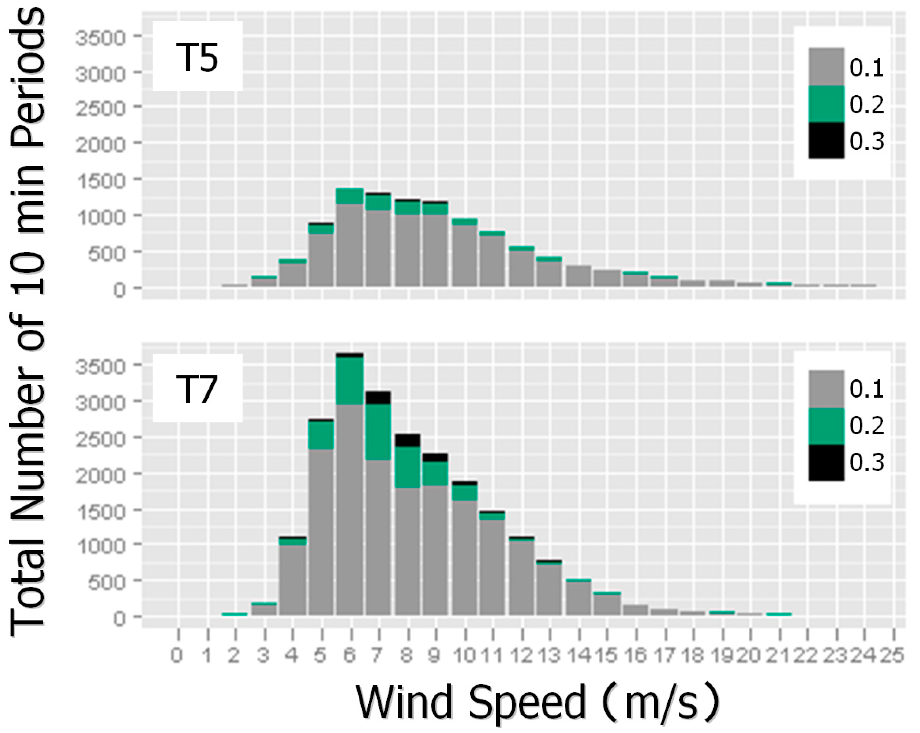
Figure 5 shows the number of 10-min periods in which the TI values evaluated from the in situ data exceeded the TI values for IEC turbulence class A at T5 and T7 in the first seven years of wind turbine operation. Figure 5 reveals that such 10-min periods occurred much more frequently at T7 than at T5. The colors used in Figure 5 indicate the amount by which the observed TI exceeded the values for IEC turbulence class A at the two wind turbine sites. The results in Figure 5 indicate that T7 was frequently affected by strong terrain-induced turbulence. Of all the wind turbines, T7 was the most frequently affected by terrain-induced turbulence that had TI values that exceeded the TI value for IEC turbulence class A (not shown due to limited space). From these findings, it can be speculated that terrain-induced turbulence was quite likely the main cause of the failures of T7.
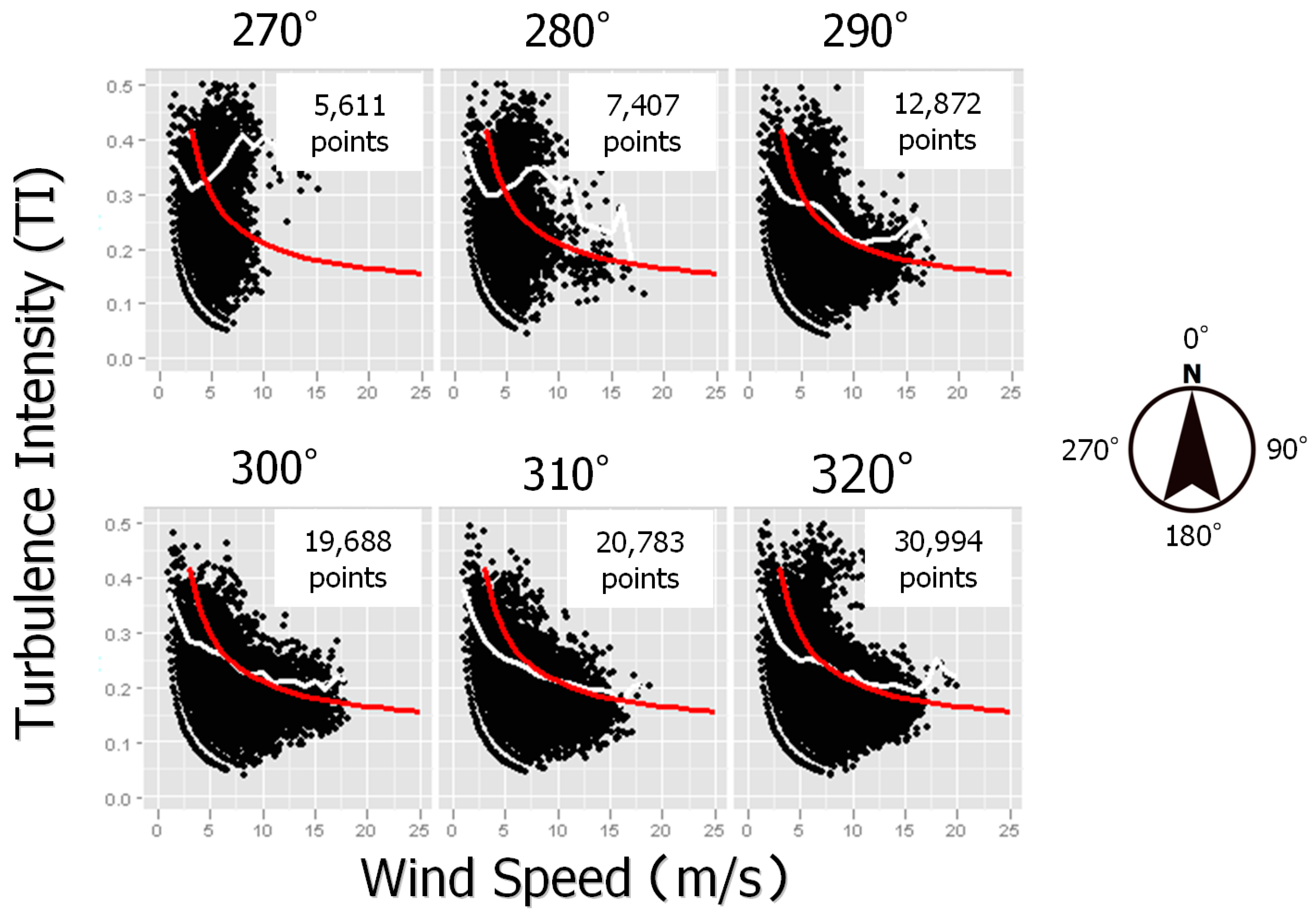
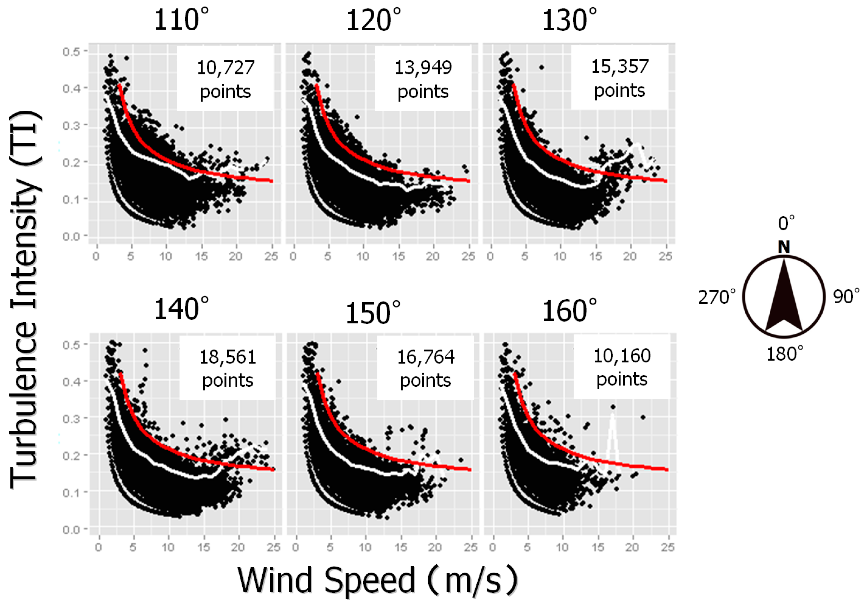
When TI values evaluated for a wind turbine are high only in some of the examined periods, it is likely that upstream terrain mainly accounts for the high values of TI in those periods and that the TI value becomes high in specific wind directions. Therefore, the values of TI for T7 were analyzed according to the wind direction. Figure 6 shows the relationship between the values of TI and wind speed at T7 for six wind directions during the first seven years of wind turbine operation. Figure 6 shows that the values of TI were high in westerly to north-westerly wind. Westerly to north-westerly wind occurred during one-third of the entire period, and such frequent occurrence of north-westerly wind is likely quite significant for T7 in terms of the increased risk of failures. (The prevailing wind direction of the area under investigation is north-westerly.) For comparison, the relationship between the values of TI and wind speed at T7 for east-south-easterly to south-south-easterly wind is shown in Figure 7. (The second most common wind direction in the area under investigation is south-easterly.) The comparisons of the TI values for different wind directions clearly revealed that terrain-induced turbulence occurred quite frequently in westerly to north-westerly wind.
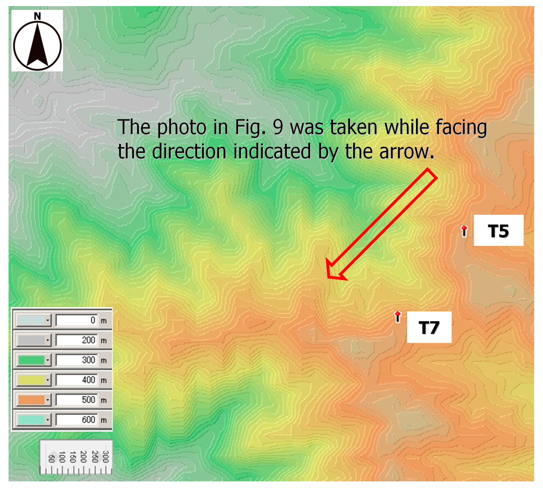
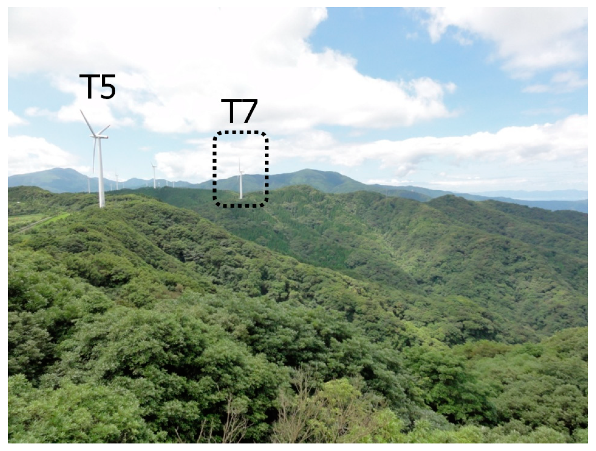
Figure 8 shows the topography in the vicinity of T7. Several ridges exist to the west and northwest of this turbine site. Figure 9 shows the ridges in the area where T7 is located. The terrain in this area is complex with large undulations. Thus, it was speculated that wind flows separated due to the ridges, and terrain-induced turbulence was generated as a result. In Section 3, the attempt to simulate this flow separation and turbulence with CFD is discussed.
3. CFD Simulation Overview
In order to closely examine the wind flow characteristics that have caused failures of the yaw gears and motors on T7, a CFD simulation was conducted. The CFD software used in the present study is RIAM-COMPACT, which was developed by the first author of the present paper. Because the details of the numerical simulation methods used in RIAM-COMPACT have been discussed in previous papers [13,14,15,16,17,18,19,20,21], they will be omitted here. In the present study, the LES is assumed to reproduce the wind tunnel testing. Therefore, the effects of atmospheric stability associated with vertical thermal stratification of the atmosphere and inflow turbulence were neglected. Thus, TI calculated from numerical results is smaller than measured data. The standard Smagorinsky model was used for the subgrid-scale model (SGS) model [22]. The model coefficient was assumed to be 0.1 by using a wall-damping function. In addition, as in [13,16,17,18], the effects of the surface roughness were taken into consideration by reconstructing surface irregularities in high resolution. A comparison between the Reynolds-averaged modeling (RANS) results and the present LES results is summarized in a recent article [14], and the prediction accuracy of the present LES approach by comparison with wind tunnel experiments is discussed in [21].
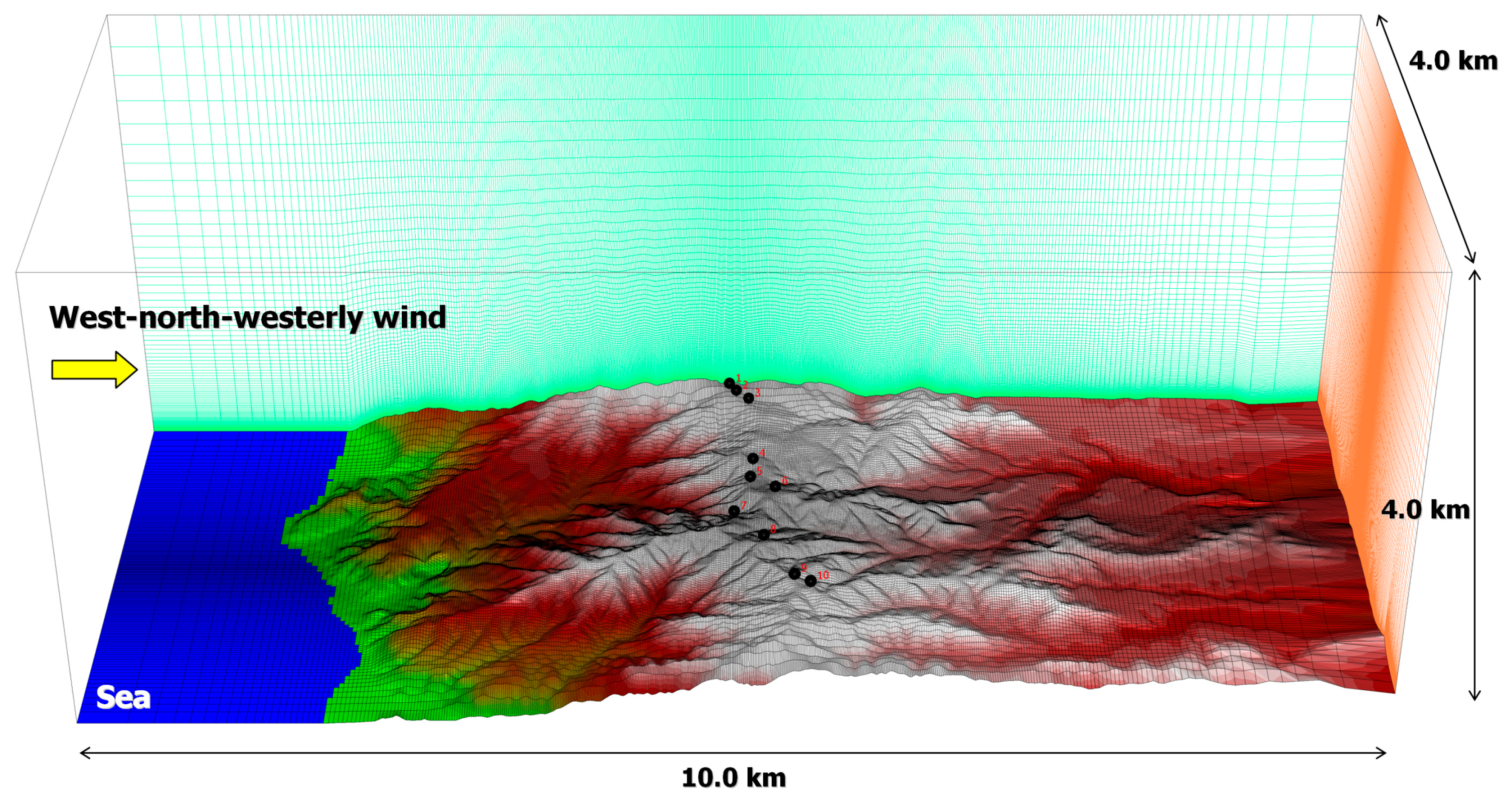
Figure 10 illustrates the computational domain and grid used for the present study. For the study, the complex terrain of the wind farm and its surroundings were numerically constructed using the 10-m resolution land surface digital elevation model (DEM) from the Geospatial Information Authority of Japan (GSI). The dimensions of the computational domain were 10.0 km × 4.0 km × 4.0 km in full scale in the streamwise (x), spanwise (y), and vertical (z) directions, respectively. The computational domain was set in such a way that T7 was located in the center of the x-y plane of the computational domain. The grid spacing for all directions varied so that grid density was high in the vicinity of T7. The minimum grid spacing for the x- and y-directions was set to approximately 8 m, and the minimum grid spacing for the z-direction was set to approximately 1.7 m. The number of grid points was 501 × 201 × 101 in the x-, y-, and z-directions, respectively, which resulted in a total number of approximately 10 million grid points. The wind direction considered for the simulation was west-north-westerly. (West-north-westerly wind is wind that flows from an angle of 292.5° clockwise from north, which was set to 0° in the wind direction coordinate system adopted in the present study.) Because inflow boundary was located over the ocean (Figure 10), the vertical wind profile of the inflow streamwise wind velocity was set according to a power law (α = 0.1, where α is the power law exponent, i.e., N = 10, where N is the inverse of α). Other boundary conditions are detailed in [13,14,15,16,17,18,19,20,21].
3.1. Results of Non-Dimensional Simulation and Discussions
The governing equations of the flow adopted in the present study (i.e., a filtered continuity equation for incompressible viscous flows and filtered Navier–Stokes equations for incompressible viscous flows) were non-dimensionalized with the use of 1) the difference between the minimum and maximum terrain elevations within the computational domain and 2) the inflow streamwise wind velocity at the height of the maximum surface elevation in the computational domain. Therefore, all the physical variables that are output by the model are non-dimensional quantities. In the current sub-section, the non-dimensional data of the three wind velocity components that were obtained from the simulation will be analyzed, and the results will be shown and discussed.
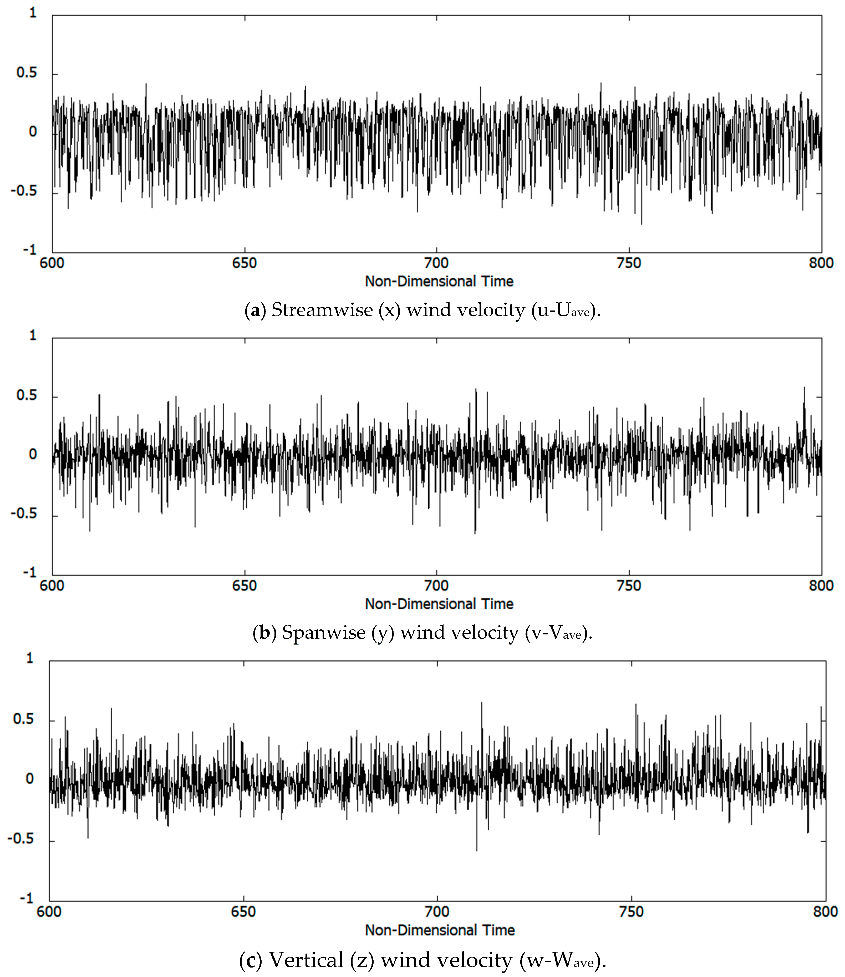
Figure 11 shows the temporal change of the fluctuating parts of the three wind velocity components at the hub height of T7 (60 m above the ground surface) in the non-dimensional time period from 600 to 800. Specifically, the data values shown for each wind velocity component are those that were obtained by subtracting the period-averaged wind velocity component from the original time series of the wind velocity component. Figure 11 shows that the values of the streamwise (x), spanwise (y), and vertical (z) wind velocity components all fluctuated significantly in time.
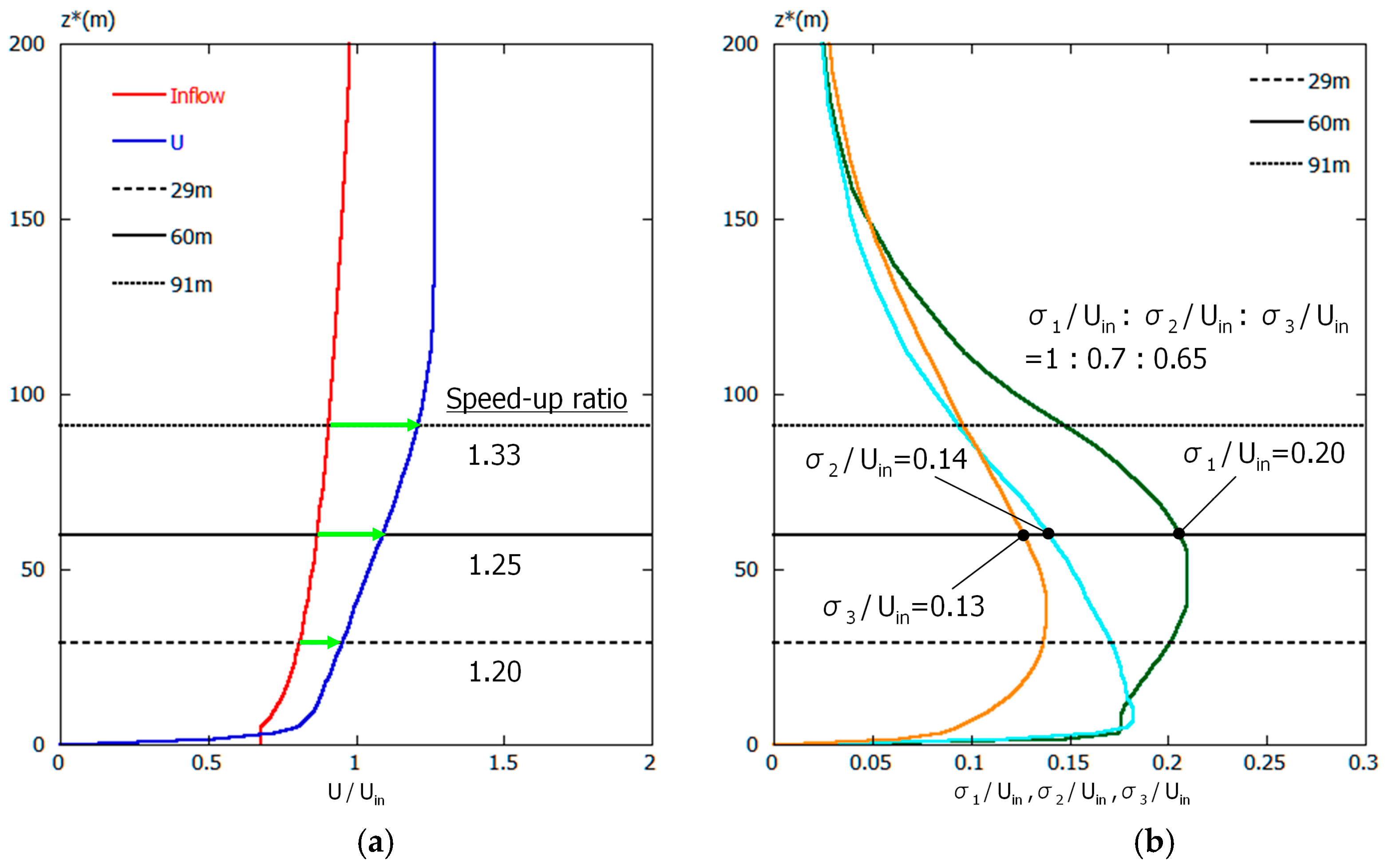
Figure 12 shows vertical profiles of statistical quantities of the turbulent flow at the site of T7 from the non-dimensional time period from 600 to 800. Figure 12a shows the vertical profiles of the streamwise wind velocity. Specifically, the red line in Figure 12 indicates the vertical profile of the streamwise inflow velocity, and the blue line indicates the vertical profile of the mean streamwise wind velocity at the site of T7 from the time period under investigation. Figure 12a also includes the values of the speed-up ratio at the bottom of the swept area (29 m above the ground surface), at the hub center (60 m above the ground surface), and at the top of the swept area (91 m above the ground surface), where the speed-up ratio is defined as the ratio of the streamwise wind velocity at a height of interest above the ground surface at the site of T7 to the inflow streamwise wind velocity at the height of interest. These results show that, due to terrain effects, the streamwise wind velocity increased locally at the wind turbine site, and additionally, there was no significant streamwise wind velocity deficit at the site. As can be presumed from Figure 10 and Figure 13, the locally increased streamwise wind velocity likely occurred as the wind flowed uphill along the terrain and into the wind turbine. Figure 12b shows the vertical profiles of the standard deviations of the streamwise (x), spanwise (y), and vertical (z) wind velocity components. The values of the standard deviations for all three components are relatively large, reflecting the temporal change of the fluctuating parts of the wind velocity components in Figure 11. Examinations of the values of the standard deviations at the hub center (60 m above the ground surface) in Figure 12b reveal that the value of the standard deviation of the vertical (z) wind velocity component is large and that the ratio of the values of the standard deviations of the three wind velocity components at the hub center was σ1:σ2:σ3 = 1.0:0.7:0.65, which clearly indicates that there was an influence of terrain-induced turbulence at this site. (This finding will be discussed again in Section 3.2).
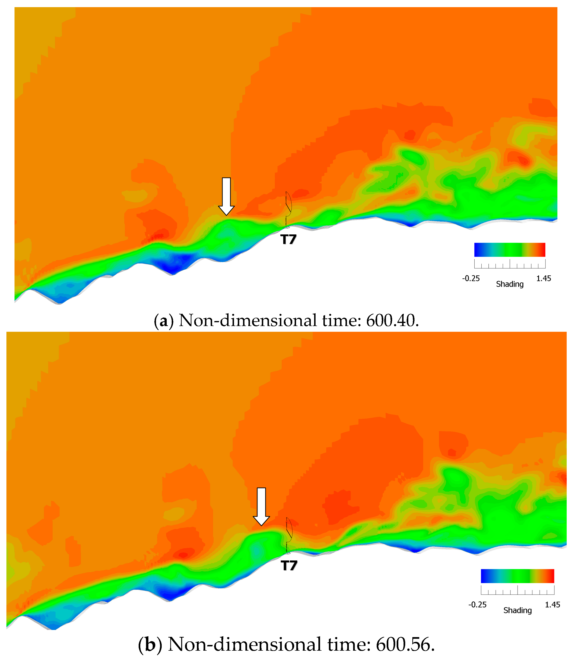
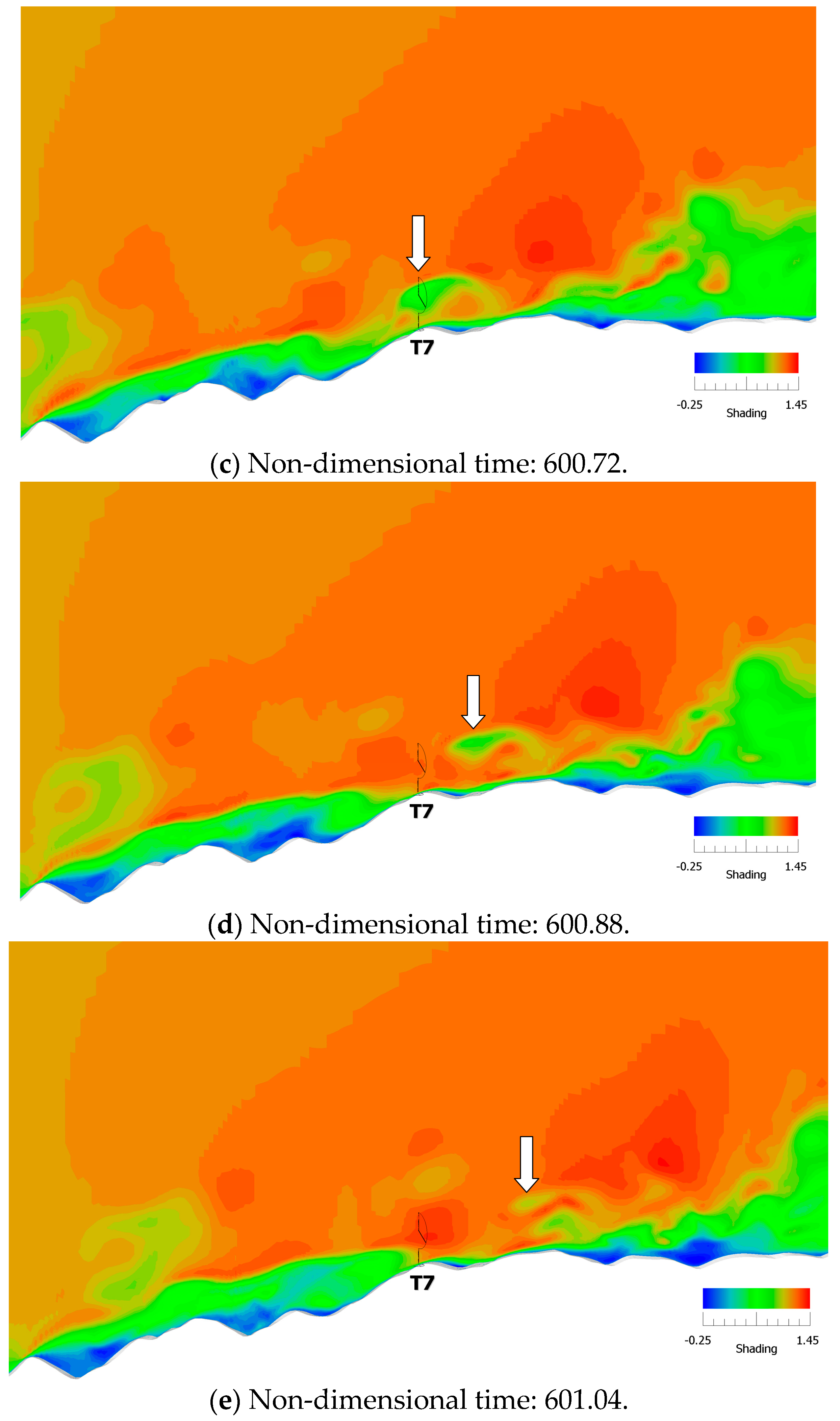
To investigate details of the flow field in the vicinity of T7, Figure 13 illustrates the temporal change of the streamwise (x) wind velocity as contour plots. The visualized streamwise wind velocity field in Figure 13 shows that, as a separation vortex (indicated by the arrows in Figure 13) that was shed upstream of the wind turbine passed through the wind turbine, the wind velocity field surrounding the wind turbine changed significantly.
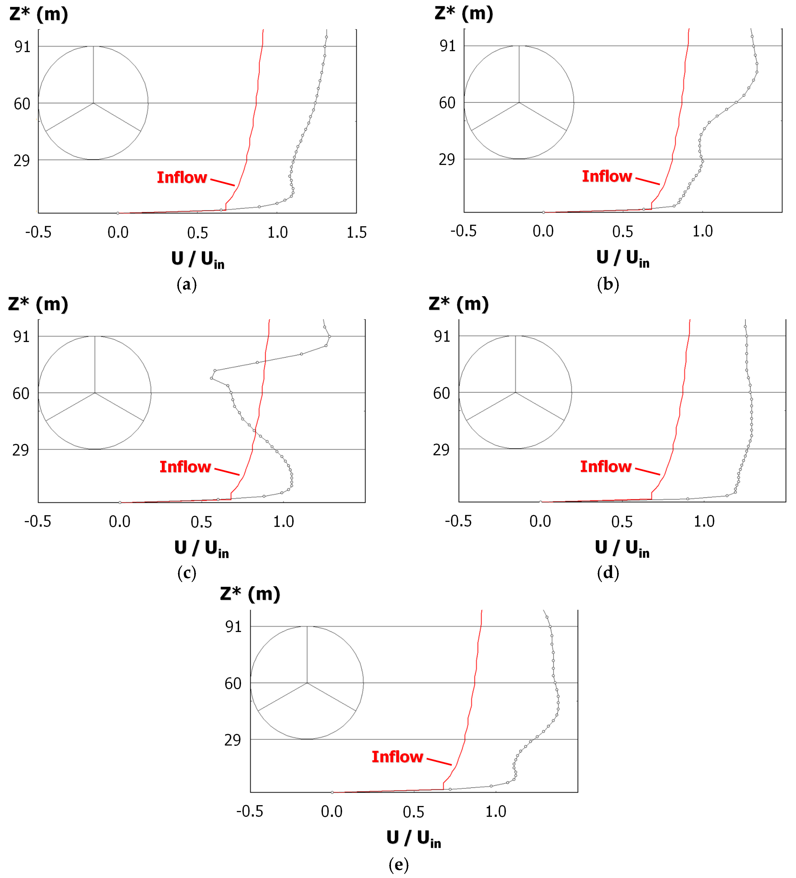
Figure 14 shows the vertical profiles of the streamwise (x) wind velocity at the site of T7 from the same times for which the cross-sectional views of the streamwise (x) wind velocity in Figure 13 were created. Immediately before the separation vortex passed through the wind turbine (Figure 13 (a)), the vertical profile of the streamwise (x) wind velocity showed a local increase of the velocity due to terrain effects and thus showed no significant wind velocity deficit with respect to the power law profile of the streamwise (x) wind velocity (Figure 14a). As the separation vortex that had been located upwind of the turbine approached the turbine, a velocity deficit occurred in the layer between the hub center (60 m above the ground surface) and the bottom of the rotor (Figure 14b). At the time at which the separation vortex arrived at the wind turbine (Figure 14c), negative wind shear was evident between the hub center height (60 m above the ground surface) and heights that were slightly higher than the hub center height. As illustrated in Figure 14d,e, after the passage of the separation vortex, the wind velocity recovered to values predicted by the power law.
A close examination of computer animations of the simulations results in Figure 13 and Figure 14 led to the following finding: The sequence of wind flow patterns described above, that is, large vortex shedding that originated from the micro-topographical features upstream of the wind turbine and its accompanying generation and disappearance of a separation vortex, occurred in a nearly periodic manner. A complex wind flow field with a vertical profile of the streamwise wind velocity such as the one in Figure 14c, which is generally rare, periodically formed in the vicinity of the wind turbine. More specifically, this vertical profile of streamwise wind velocity deviated significantly from the power law and also had negative wind shear. It can be surmised that when complex wind flow with such a profile passes through a wind turbine, it causes a large wind load on the turbine. In addition, because the structure of the abovementioned complex wind flow is three-dimensional, wind loads on the left and right side of the swept area of a wind turbine in such a wind flow are expected to differ. Thus, it can be speculated that such wind loads would exert force on the wind turbine in such a way that they would forcibly rotate the nacelle of the wind turbine, which in turn would cause impact loads on both the yaw gears and motors and result in the failures of the yaw gears and motors in the end. Accordingly, it may be possible to make prior assessments of wind turbine failure risks due to terrain-induced turbulence by studying, with the use of CFD, wind velocity fluctuations in the vicinity of a wind turbine and the vertical profiles of statistical quantities of the three velocity components (i.e., the three-dimensional flow structure) within the swept area.
3.2. Re-Scaled Dimensional Simulation Results and Discussions
The temporal change of the streamwise (x) wind velocity (a non-dimensional quantity) in the period from 600 to 800 in non-dimensional time at the hub height of T7 was re-scaled such that the average value of the streamwise (x) wind velocity at the hub height of this turbine for this period became 8.0 m/s. The abovementioned re-scaling procedure can be summarized as follows:
- (1)
- The average value of the streamwise (x) wind velocity (a non-dimensional quantity) at the hub height of T7 was calculated for the period from 600 to 800 in non-dimensional time. The calculated average value was 1.087 in the present study.
- (2)
- A correction coefficient was calculated so that the average value of the streamwise (x) wind velocity at the hub height of T7 in the period under investigation was 8.0 m/s in full scale. Then, the non-dimensional wind velocity data from the entire simulation time period were multiplied by the calculated correction coefficient. The calculated correction coefficient was 7.36 (= 8.0/1.087) in the present study. With this procedure, the streamwise (x) non-dimensional wind velocity was converted to full-scale wind velocity (m/s).
- (3)
- The time in the period from 600 to 800 in non-dimensional time was converted to full scale using the equation T = t (h/Uin), where T is full-scale time (s), t is non-dimensional time, h is the difference between the minimum and maximum terrain elevations within the computational domain (m), and Uin is the streamwise wind velocity (m/s) at the height of the maximum surface elevation in the computational domain at the inflow boundary. In the present study, the 200 non-dimensional time period, i.e., the period from 600 to 800 in non-dimensional time, was converted to approximately 15,500 s (approximately 4 h) in full scale. The time step was 0.3 s in full scale.
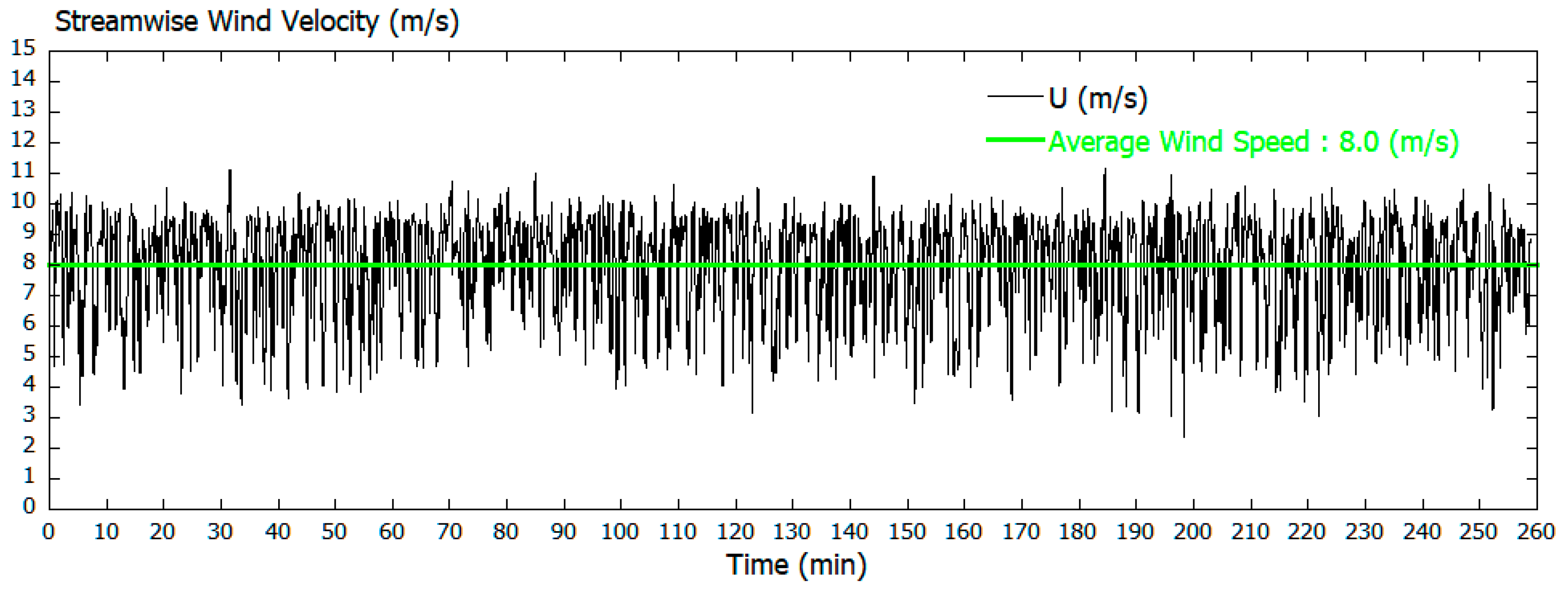
Figure 15 shows the temporal change of the full-scale streamwise (x) wind velocity (m/s) that was obtained from the rescaling procedure with the method described above (total data points: 50,000; time interval: 0.3 s). The green line in the figure indicates 8.0 m/s, which is the average streamwise (x) wind velocity that the re-scaling procedure was designed to attain for the hub height of T7 in the time period under investigation.
Figure 16 shows a histogram of the streamwise (x) wind velocity data from Figure 15 with bin widths of 1 m/s. The average streamwise (x) wind velocity that the re-scaling procedure was designed to attain for the time period investigated was 8.0 m/s in the present study. As a result, the re-scaled streamwise (x) wind velocity ranged between approximately 4.0 and 11.0 m/s, and the occurrence frequency of the wind velocity class of 9.0 to 10.0 m/s in particular was large.
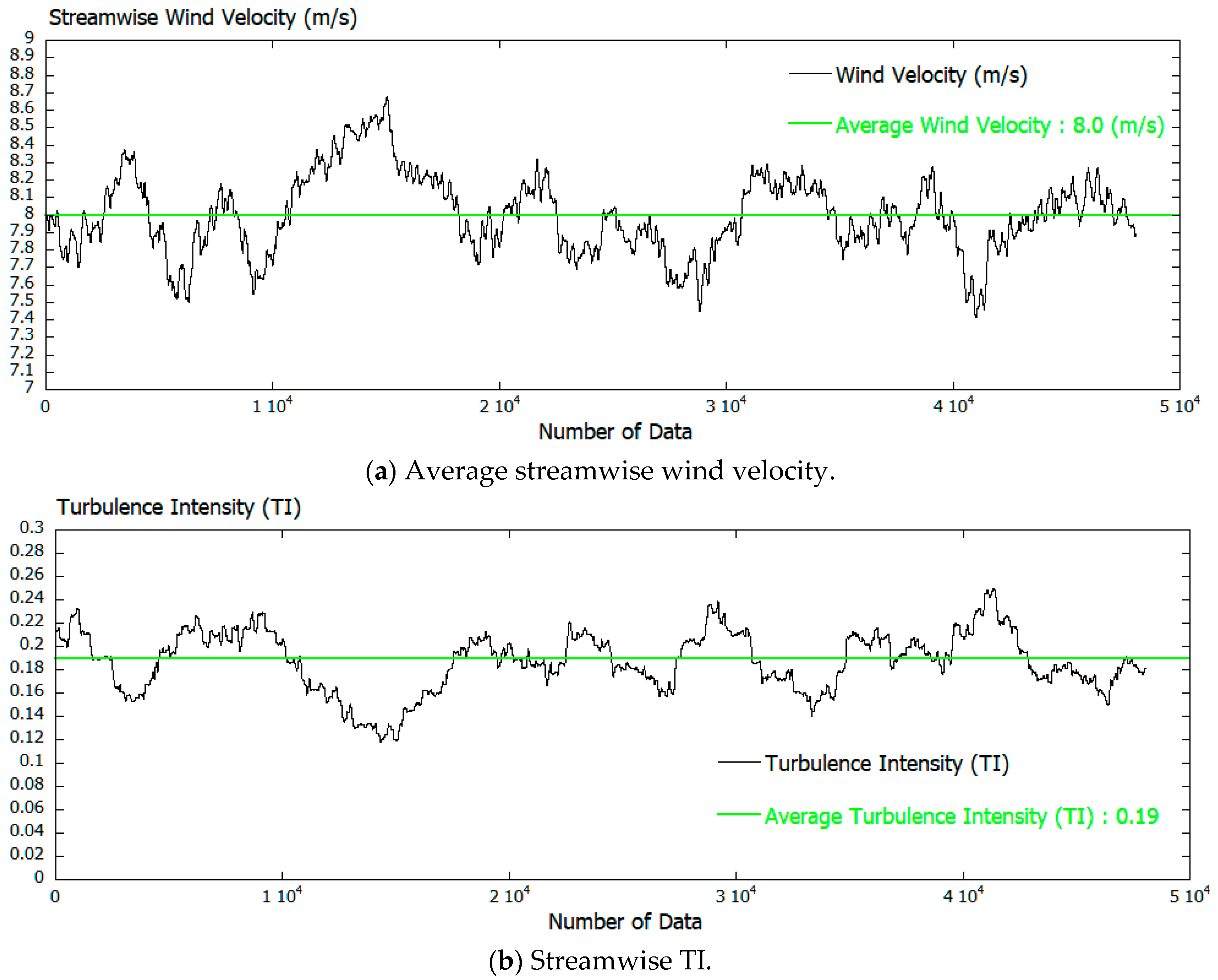
In the present study, following a common statistical processing procedure adopted for in situ data, a 10-min moving average filter (1932-point averaging filter) was applied to the time series of the re-scaled streamwise (x) wind velocity (m/s) in Figure 15 (total data points: 50,000; time interval: 0.3 s) to evaluate the values of the moving-averaged wind velocity and the corresponding TI (Figure 17) (48,068 data points). In Figure 17a, the green line indicates 8.0 m/s, which is the average streamwise wind velocity (x) that the re-scaling procedure in this study was designed to attain for the time period under investigation. Figure 17b shows the evaluated TI values. These values were obtained with Equation (1) below using a moving-averaged filter with a window length of 10-min and the wind velocity data within the window (number of sample data points: 1932).
where
where u(t) is the instantaneous streamwise wind velocity, is the average of the instantaneous streamwise wind velocity within the 10-min moving-averaged window, and u’ is the fluctuating component of the streamwise wind velocity due to turbulence. Figure 17a,b shows that the values of the average streamwise velocity and TI fluctuate in a correlated manner.
That is, as the average wind velocity in Figure 17a increases, the TI in Figure 17b decreases. Conversely, as the average wind velocity in Figure 17a decreases, the TI in Figure 17b increases. A further examination of the temporal change of the TI in Figure 17b reveals that the TI changes in large amplitude with the increasing and decreasing average wind velocity. The average value of TI was 0.19 (the green line in Figure 17b), which is relatively large. This result also indicates that T7 was strongly affected by terrain-induced turbulence.
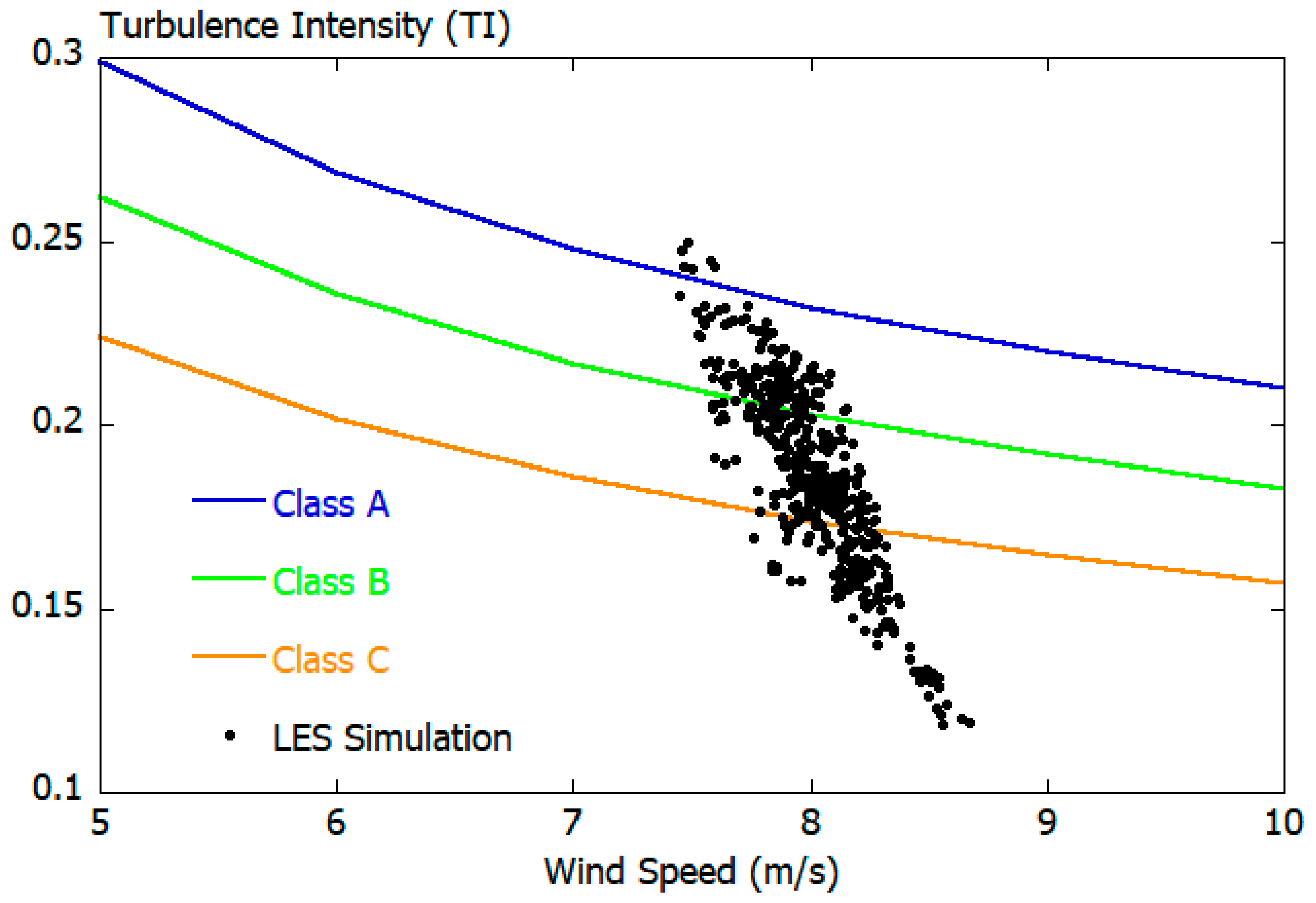
Finally, the TI values from Figure 17 were examined by comparing them with those from the NTM in IEC 61400-1 Ed.3 (2005) (Figure 18). The NTM defines wind turbine classes as in Table 1. Vref in Table 1 represents the 50-year return period values of 10-min average wind speed. Iref is the expected value of TI for a wind speed of 15 m/s.
For NTM, the values of and and are calculated using the streamwise (x) wind velocity as
where Iref is the expected value for the turbulence intensity for V = 15 m/s; TI is the turbulence intensity; U is the 10-min average streamwise wind velocity (m/s); σ is wind velocity standard deviation (m/s); and subscript 90q is the 0.9 quantile value.
Wind turbine designers design wind turbines in such a way that they meet both the wind turbine class and turbulence class requirements. Wind power providers are able to reduce their business risks by confirming that the values of TI at their wind turbine sites lie under the curve defined by Equation (4). Figure 18 shows that the values of the streamwise (x) TI simulated with the abovementioned method were not as large as those observed in situ (Figure 6). However, some of the simulated values exceeded the TI values for turbulence class A, suggesting that the influence of terrain-induced turbulence on the wind turbine was well simulated.
Based on turbulence spectral relationships, the spanwise (y) wind-velocity standard deviation, σ2, and the vertical (z) wind-velocity standard deviation, σ3, are given with respect to the streamwise (x) wind-velocity standard deviation, σ1, as in Equations (5) and (6). Both of these equations were derived from turbulence spectra from wind flow over flat terrain.
In the present study, the value of the standard deviation of the vertical (z) wind velocity, σ3, at the hub height of T7 in Figure 12b was fairly large as discussed earlier and shown below:
4. Conclusions
The first part of the present study investigated the relationship among the number of yaw gear and motor failures and TI at all the wind turbines under investigation with the use of in situ data. The investigation revealed that wind turbine #7 (T7), which experienced a large number of failures, was affected by terrain-induced turbulence with TI that exceeded those presumed for the wind turbine design class for which T7 was designed. The frequency of occurrence of such terrain-induced turbulence at this wind turbine was also significantly higher than that at the other wind turbines. When the TI values evaluated for a wind turbine are high only in some of the examined periods, it is likely that upstream terrain mainly accounts for the high values in those periods and that the TI values become high in specific wind directions. Accordingly, the TI values at T7 were examined with respect various wind directions. The examination revealed that the TI values were high in westerly to northwesterly winds. Because complex terrain with ridges and surface undulations of various scales exists in the vicinity of T7, it was speculated that wind flows separated due to these ridges, resulting in terrain-induced turbulence.
Subsequently, a CFD simulation was performed to examine if the abovementioned observed wind flow characteristics could be successfully simulated. The CFD software package that was used in the present study was RIAM-COMPACT, which was developed by the first author of the present paper. RIAM-COMPACT is a nonlinear, unsteady wind prediction model that uses LES for the turbulence model. RIAM-COMPACT is capable of simulating flow collision, separation, and reattachment and also various unsteady turbulence–eddy phenomena that are caused by flow collision, separation, and reattachment. A close examination of computer animations of the streamwise (x) wind velocity revealed the following findings: As we predicted, wind flow that was separated from a micro-topographical feature (micro-scale terrain undulations) upstream of T7 generated large vortices. These vortices were shed downstream in a nearly periodic manner, which in turn generated terrain-induced turbulence, affecting T7 directly. In addition, vertical wind profiles of the (instantaneous) streamwise wind velocity at the wind turbine site were studied from the time at which the abovementioned unsteady turbulence–eddy phenomena occurred. As a result, it was found that a complex wind flow field with unusual vertical profiles of streamwise wind velocity formed at the wind turbine. More specifically, these vertical profiles of streamwise wind velocity deviated significantly from the power law profile and also had negative wind shear. On the other hand, the time-averaged wind flow data showed that the average streamwise wind velocity increased locally at the wind turbine site due to terrain effects and that no significant wind velocity deficit occurred at the site. Thus, even when no significant wind velocity deficit existed in the vertical profile of the time-averaged streamwise wind velocity, significant velocity deficits were present in vertical profiles of the instantaneous wind velocity, and such instantaneous wind velocity deficits should not be overlooked. An examination of the values of the standard deviations of the three wind velocity components at the wind turbine hub center (60 m above the ground surface) revealed that the value for the vertical (z) direction was large. The ratio of the standard deviations of the three wind velocity components at the wind turbine hub height was σ1:σ2:σ3 = 1.0:0.7:0.65, which clearly showed the effect of terrain-induced turbulence. When wind flow with such properties passes through a wind turbine, it causes a large wind load on the wind turbine. Furthermore, because the structure of this complex wind flow is three-dimensional, wind loads imposed on the left and right side of the swept area are expected to differ. It was speculated that such wind loads would exert force on the wind turbine in such a way that they would forcibly rotate the nacelle of the wind turbine, which in turn would cause impact loads on both the yaw gears and motors and ultimately result in the failures of the yaw gears and motors.
Finally, the temporal change of the streamwise (x) wind velocity (a non-dimensional quantity) at the hub height of T7 in the period from 600 to 800 in non-dimensional time was re-scaled in such a way that the average value of the streamwise (x) wind velocity for this period was 8.0 m/s, and the results of the analysis of the re-scaled data were discussed. With the re-scaled full-scale streamwise wind velocity (m/s) data (total number of data points: approximately 50,000; time interval: 0.3 s), the time-averaged streamwise (x) wind velocity and turbulence intensity (TI) were evaluated using a common statistical processing procedure adopted for in situ data. Specifically, 10-min moving averaging (number of sample data points: 1932) was performed on the re-scaled data. Comparisons of the evaluated TI values to the TI values from the Normal Turbulence Model in IEC61400-1 Ed.3 (2005) revealed the following: Although the evaluated TI values were not as large as those observed in situ, some of the evaluated TI values exceeded the values for turbulence class A, suggesting that the influence of terrain-induced turbulence on the wind turbine was well simulated.
Author Contributions
The study idea, plan and design were conceived by T.U.; And, all authors prepared the manuscript.
Funding
This work was supported by JSPS KAKENHI Grant Number 17H02053.
Acknowledgments
The present study was supported by collaborative research with Eurus Energy Holdings Corporation: (1) Collaborative research and development on a method for assessing the wind speed ratio for wind turbine sites on complex terrain, July 2013-March 2014, December 2015-March 2018; (2) Collaborative research on land use modeling and its effect on simulated local-scale wind fields, December 2015-June 2016, principle investigator: Takanori Uchida. The authors wish to express their gratitude to all the individuals involved.
Conflicts of Interest
All authors declare no conflict of interest.
References
- Rodrigues, R.V.; Lengsfeld, C. Development of a Computational System to Improve Wind Farm Layout, Part I: Model Validation and Near Wake Analysis. Energies 2019, 12, 940. [Google Scholar] [CrossRef]
- Gargallo-Peiró, A.; Avila, M.; Owen, H.; Prieto-Godino, L.; Folch, A. Mesh generation, sizing and convergence for onshore and offshore wind farm Atmospheric Boundary Layer flow simulation with actuator discs. J. Comput. Phys. 2018, 375, 209–227. [Google Scholar] [CrossRef]
- Sessarego, M.; Shen, W.Z.; Van der Laan, M.P.; Hansen, K.S.; Zhu, W.J. CFD Simulations of Flows in a Wind Farm in Complex Terrain and Comparisons to Measurements. Appl. Sci. 2018, 8, 788. [Google Scholar] [CrossRef]
- Temel, O.; Bricteux, L.; van Beeck, J. Coupled WRF-OpenFOAM study of wind flow over complex terrain. J. Wind Eng. Ind. Aerodyn. 2018, 174, 152–169. [Google Scholar] [CrossRef]
- Castellani, F.; Buzzoni, M.; Astolfi, D.; D’Elia, G.; Dalpiaz, G.; Terzi, L. Wind Turbine Loads Induced by Terrain and Wakes: An Experimental Study through Vibration Analysis and Computational Fluid Dynamics. Energies 2017, 10, 1839. [Google Scholar] [CrossRef]
- Murthy, K.S.R.; Rahi, O.P. A comprehensive review of wind resource assessment. Renew. Sustain. Energy Rev. 2017, 72, 1320–1342. [Google Scholar] [CrossRef]
- Simões, T.; Estanqueiro, A. A new methodology for urban wind resource assessment. Renew. Energy 2016, 89, 598–605. [Google Scholar] [CrossRef] [Green Version]
- Gopalan, H.; Gundling, C.; Brown, K.; Roget, B.; Sitaraman, J.; Mirocha, J.D.; Miller, W.O. A coupled mesoscale-microscale framework for wind resource estimation and farm aerodynamics. J. Wind Eng. Ind. Aerodyn. 2014, 132, 13–26. [Google Scholar] [CrossRef]
- Ishugah, T.F.; Li, Y.; Wang, R.Z.; Kiplagat, J.K. Advances in wind energy resource exploitation in urban environment: A review. Renew. Sustain. Energy Rev. 2014, 37, 613–626. [Google Scholar] [CrossRef]
- Porté-Agel, F.; Wu, Y.-T.; Chen, C.-H. A Numerical Study of the Effects of Wind Direction on Turbine Wakes and Power Losses in a Large Wind Farm. Energies 2013, 6, 5297–5313. [Google Scholar] [CrossRef] [Green Version]
- Gasset, N.; Landry, M.; Gagnon, Y. A Comparison of Wind Flow Models for Wind Resource Assessment in Wind Energy Applications. Energies 2012, 5, 4288–4322. [Google Scholar] [CrossRef] [Green Version]
- Palma, J.M.L.M.; Castro, F.A.; Ribeiro, L.F.; Rodrigues, A.H.; Pinto, A.P. Linear and nonlinear models in wind resource assessment and wind turbine micro-siting in complex terrain. J. Wind Eng. Ind. Aerodyn. 2008, 96, 2308–2326. [Google Scholar] [CrossRef] [Green Version]
- Uchida, T. Numerical Investigation of Terrain-induced Turbulence in Complex Terrain by Large-eddy Simulation (LES) Technique. Energies 2018, 11, 2638. [Google Scholar] [CrossRef]
- Uchida, T.; Li, G. Comparison of RANS and LES in the Prediction of Airflow Field over Steep Complex Terrain. Open J. Fluid Dyn. 2018, 8, 286–307. [Google Scholar] [CrossRef]
- Uchida, T. Computational Investigation of the Causes of Wind Turbine Blade Damage at Japan’s Wind Farm in Complex Terrain. J. Flow Control Meas. Vis. 2018, 6, 152–167. [Google Scholar] [CrossRef]
- Uchida, T. Computational Fluid Dynamics Approach to Predict the Actual Wind Speed over Complex Terrain. Energies 2018, 11, 1694. [Google Scholar] [CrossRef]
- Uchida, T. LES Investigation of Terrain-Induced Turbulence in Complex Terrain and Economic Effects of Wind Turbine Control. Energies 2018, 11, 1530. [Google Scholar] [CrossRef]
- Uchida, T. Computational Fluid Dynamics (CFD) Investigation of Wind Turbine Nacelle Separation Accident over Complex Terrain in Japan. Energies 2018, 11, 1485. [Google Scholar] [CrossRef]
- Uchida, T. Large-Eddy Simulation and Wind Tunnel Experiment of Airflow over Bolund Hill. Open J. Fluid Dyn. 2018, 8, 30–43. [Google Scholar] [CrossRef]
- Uchida, T.; Ohya, Y. Latest Developments in Numerical Wind Synopsis Prediction Using the RIAM-COMPACT® CFD Model. Energies 2011, 4, 458–474. [Google Scholar] [CrossRef]
- Uchida, T.; Ohya, Y. Micro-siting technique for wind turbine generators by using large-eddy simulation. J. Wind Eng. Ind. Aerodyn. 2008, 96, 2121–2138. [Google Scholar] [CrossRef]
- Smagorinsky, J. General circulation experiments with the primitive equations. Part 1, Basic experiments. Mon. Weather Rev. 1963, 91, 99–164. [Google Scholar] [CrossRef]
Figure 1.
General view of the wind warm under investigation. (T1–T16 indicate the locations of wind turbines #1–#16).
Figure 1.
General view of the wind warm under investigation. (T1–T16 indicate the locations of wind turbines #1–#16).

Figure 2.
Comparison of the number of yaw gear and motor failures at all the wind turbines.

Figure 3.
Yaw gear damage at wind turbine #7 (T7).

Figure 4.
Comparison between the turbulence intensity (TI) at wind turbine #5 (T5) and that at T7. The data plotted here are those that were collected during the first year of the wind turbine operation. The numbers in the upper right indicate the number of plotted data values. The red lines indicate the relationship between TI and wind speed for International Electrotechnical Commission (IEC) turbulence class A. The white lines indicate the sum of the bin average and one bin standard deviation (σ) of the plotted TI values.

Figure 5.
Comparison of the number of 10-min periods in which the TI of terrain-induced turbulence exceeded that for IEC turbulence class A at T5 and T7.
Figure 5.
Comparison of the number of 10-min periods in which the TI of terrain-induced turbulence exceeded that for IEC turbulence class A at T5 and T7.

Figure 6.
TI at T7 in westerly to north-westerly wind. The plot in the upper left panel is for a wind direction of 270°, and the plot in the lower right panel is for a wind direction of 320°.
Figure 6.
TI at T7 in westerly to north-westerly wind. The plot in the upper left panel is for a wind direction of 270°, and the plot in the lower right panel is for a wind direction of 320°.

Figure 7.
TI at T7 in east-south-easterly to south-south-easterly wind. The plot in the upper left panel is for a wind direction of 110°, and the plot in the lower right panel is for a wind direction of 160°.
Figure 7.
TI at T7 in east-south-easterly to south-south-easterly wind. The plot in the upper left panel is for a wind direction of 110°, and the plot in the lower right panel is for a wind direction of 160°.

Figure 8.
Topography in the vicinity of T7.

Figure 9.
Photo of the area where T7 is located.

Figure 10.
Computational domain and grid used for the present study.

Figure 11.
Temporal change of the fluctuating parts of the wind velocity components at the hub height (60 m above the ground surface) of T7.
Figure 11.
Temporal change of the fluctuating parts of the wind velocity components at the hub height (60 m above the ground surface) of T7.

Figure 12.
Vertical profiles of statistical quantities of the turbulent flow at the site of T7. (a) Normalized mean streamwise wind velocity; (b) Normalized standard deviation of the three wind velocity components. (Uin: the inflow streamwise wind velocity at the height of the maximum surface elevation in the computational domain. z*(m): the height above the ground.)

Figure 13.
Temporal change of the streamwise (x) wind velocity field in the vertical cross-section that includes the site of T7.
Figure 13.
Temporal change of the streamwise (x) wind velocity field in the vertical cross-section that includes the site of T7.


Figure 14.
Temporal change in the vertical profile of the streamwise (x) wind velocity at the site of T7. The profiles in (a–e) correspond to the vertical cross-sectional views of the streamwise (x) wind velocity field shown in Figure 13a–e. (a) Non-dimensional time: 600.40, (b) Non-dimensional time: 600.56, (c) Non-dimensional time: 600.72; (d) Non-dimensional time: 600.88, (e) Non-dimensional time: 601.04. (z*(m): the height above the ground.)

Figure 15.
Temporal change of the streamwise (x) wind velocity at the hub height of T7 (60 m above the ground surface) that was rescaled to full scale (m/s).
Figure 15.
Temporal change of the streamwise (x) wind velocity at the hub height of T7 (60 m above the ground surface) that was rescaled to full scale (m/s).

Figure 16.
Frequency distribution of the streamwise (x) wind velocity that has been rescaled to full scale (m/s) for the time period shown in Figure 15.
Figure 16.
Frequency distribution of the streamwise (x) wind velocity that has been rescaled to full scale (m/s) for the time period shown in Figure 15.

Figure 17.
Temporal change of the full-scale streamwise (x) wind velocity (m/s) and TI. Both are calculated by applying a moving-averaged window to the time series data in Figure 15. The data shown are for the hub height (60 m above the ground surface) at T7.
Figure 17.
Temporal change of the full-scale streamwise (x) wind velocity (m/s) and TI. Both are calculated by applying a moving-averaged window to the time series data in Figure 15. The data shown are for the hub height (60 m above the ground surface) at T7.

Figure 18.
The relationship between TI and wind speed in the location of T7 at hub height (60 m above the ground surface). Dots: Simulation results from the present study. The plotted data were extracted every 100 data points from the time series of TI calculated from the simulation data. Lines: IEC turbulence categories A, B, and C from the NTM, defined in IEC 61400-1 Ed.3 (2005).


Table 1.
Wind turbine class according to IEC 61400-1 Ed.3 (2005).
| Class | Ⅰ | Ⅱ | Ⅲ | S | |
|---|---|---|---|---|---|
| Vref | 50.0 | 42.5 | 37.5 | Values specified by the designer | |
| Iref | A | 0.16 | |||
| B | 0.14 | ||||
| C | 0.12 | ||||
© 2019 by the authors. Licensee MDPI, Basel, Switzerland. This article is an open access article distributed under the terms and conditions of the Creative Commons Attribution (CC BY) license (http://creativecommons.org/licenses/by/4.0/).
Share and Cite
MDPI and ACS Style
Uchida, T.; Takakuwa, S. A Large-Eddy Simulation-Based Assessment of the Risk of Wind Turbine Failures Due to Terrain-Induced Turbulence over a Wind Farm in Complex Terrain. Energies 2019, 12, 1925. https://doi.org/10.3390/en12101925
AMA Style
Uchida T, Takakuwa S. A Large-Eddy Simulation-Based Assessment of the Risk of Wind Turbine Failures Due to Terrain-Induced Turbulence over a Wind Farm in Complex Terrain. Energies. 2019; 12(10):1925. https://doi.org/10.3390/en12101925
Chicago/Turabian StyleUchida, Takanori, and Susumu Takakuwa. 2019. "A Large-Eddy Simulation-Based Assessment of the Risk of Wind Turbine Failures Due to Terrain-Induced Turbulence over a Wind Farm in Complex Terrain" Energies 12, no. 10: 1925. https://doi.org/10.3390/en12101925
Note that from the first issue of 2016, this journal uses article numbers instead of page numbers. See further details here.