Observation of Near-Inertial Oscillations Induced by Energy Transformation during Typhoons

1
Key Laboratory of Ocean Circulation and Wave Studies, Institute of Oceanology, Chinese Academy of Sciences, Qingdao 266071, China
2
University of Chinese Academy of Sciences, Beijing 100049, China
3
Nanjing University of Information Science and Technology, Nanjing 210044, China
*
Authors to whom correspondence should be addressed.
Energies 2019, 12(1), 99; https://doi.org/10.3390/en12010099
Submission received: 19 October 2018
/
Revised: 22 December 2018
/
Accepted: 25 December 2018
/
Published: 29 December 2018
Abstract
:Three typhoon events were selected to examine the impact of energy transformation on near-inertial oscillations (NIOs) using observations from a subsurface mooring, which was deployed at 125° E and 18° N on 26 September 2014 and recovered on 11 January 2016. Almost 16 months of continuous observations were undertaken, and three energetic NIO events were recorded, all generated by passing typhoons. The peak frequencies of these NIOs, 0.91 times of the local inertial frequency f, were all lower than the local inertial frequency f. The estimated vertical group velocities (Cgz) of the three NIO events were 11.9, 7.4, and 23.0 m d−1, and were relatively small compared with observations from other oceans (i.e., 100 m d−1). The directions of the horizontal near-inertial currents changed four or five times between the depths of 40 and 800 m in all three NIO events, implying that typhoons in the northwest Pacific usually generate high-mode NIOs. The NIO currents were further decomposed by performing an empirical orthogonal function (EOF) analysis. The first and second EOF modes dominated the NIOs during each typhoon, accounting for more than 50% of the total variance. The peak frequencies of the first two EOF modes were less than f, but those of the third and fourth modes were higher than f. The frequencies of all the modes during non-typhoon periods were more than f. Our analysis indicates that the relatively small downward group velocity was caused by the frequent direction changes of the near-inertial currents with depth.
1. Introduction
Free-propagating internal waves in the ocean usually have frequencies lower than the buoyancy frequency N and higher than the inertial frequency f [1,2]. Near-inertial oscillations (NIOs) are internal waves with frequencies close to the local inertial frequency f. NIOs have been observed in all ocean basins and the entire ocean column [3,4,5]. The breaking of near-inertial waves can cause ocean mixing, which influences pollutant dispersal and marine productivity [3,6,7], maintains ocean thermohaline circulation, and modulates the climate [8]. Alford presented spatial maps of wind–NIO energy fluxes [8] between 50° S and 50° N, which showed that the energy supplied to NIOs by wind is of the same order of magnitude as that provided to baroclinic tides by their barotropic counterparts. NIOs are strongly intermittent or highly temporally variable [9] and have high wavenumber aspects [10,11,12]. NIOs may play an important role in upper-ocean mixing, potentially affecting various processes, including the biogeochemical variety and those affecting the climate [13].
Near-inertial waves are largely generated by transient strong wind systems, such as mid-latitude storms and tropical cyclones, while NIOs have been observed in all ocean basins [14,15,16]. Strong winds supply kinetic energy to the mixed layer of the ocean, generating strong currents. Near-inertial internal waves form after several Rossby adjustment cycles [17,18]. Strong vertical shear in a near-inertial horizontal current can cause intense turbulent mixing at the base of the mixed layer through shear instability, which can entrain subsurface cold water, bringing it to the sea surface and markedly cooling the latter under a typhoon [7,19,20]. This cooling can further decrease or even eliminate surface enthalpy fluxes from the ocean to the atmosphere, significantly affecting typhoon evolution and intensity changes. Fluctuations in tropical cyclones, that is, negative feedback from the ocean, can therefore occur [21]. Clockwise-rotating energy peaks at near-inertial frequencies for records from all current meter mooring accompanying the passage of atmospheric fronts was found by Chen in the Texas-Louisiana shelf [22]. Studies of typhoon-generated NIOs have been focused on observations made under high wind conditions to allow forecasting of the typhoon’s intensity to be improved, for example, in the Gulf of Mexico [23,24] and the Atlantic [16].
Near-inertial kinetic energy (NIKE) is generated in the surface mixed layer before being preferentially propagated from thence to the deep ocean [25,26,27,28], providing the energy for thermohaline circulation to occur [29]. NIOs propagate downward decay because of turbulent dissipation. Alford and Whitmont [30] examined 2,480 historical current-meter records and found that NIKE decreased by a factor of 4–5 between depths of 500 and 3,500 m in winter. Eugene found that wind-generated, near-inertial, internal waves reach a depth of 1200 m (where many current meters were located) in a few days after the hurricane passes the region [31]. Meanwhile, Alford et al. [32] found that 12%–33% of the surface NIKE could reach a depth of 800 m at the Papa station in the northeast Pacific Ocean. The vertical group velocity Cgz of an NIO depends theoretically on the vertical wave number m and becomes extremely small when the NIO has a large m, resulting in sizable differences between the group velocities Cgz of NIOs, as has been found in numerous previous studies (see Table 1).
As shown in Table 1, vertical propagation of NIKE was examined using in situ observations or numerical simulation in previous studies [18,19]. Qi et al. [18] used the observations of two moorings in the northeast Pacific Ocean to calculate the vertical group velocity in different months. The fastest was in October by mooring Cl; the slowest was in March by mooring NP. The Pacific is the largest ocean in the world. Many studies have focused on NIO events therein, including Alford [3], who estimated that the north Pacific receives an annual mean energy input of 65 ± 10 GW from wind over the box of calculation (13% of the total energy input from wind for all the oceans). Energetic NIOs have been observed at all depths in the eastern Pacific, radiating both upward and downward in abrupt ridges/steps, with near-inertial shear exceeding internal tide shear by a factor of 2–4 at all depths [12]. Furthermore, shallow ocean near-inertial wave responses to three typhoons in the north-western South China Sea were examined using temperature and current profiles observed at moorings in 2005 [5]. Kim et al. [33] found that an anti-cyclonic eddy trapped near-inertial energy between two layers at depths of 120–210 m in the northwest Pacific. This region suffers more frequent and intense typhoons than any other oceanic zone and features highly complex current systems, such as the Kuroshio and the Northern Equatorial Currents [36,37], although few in-situ observations of NIOs have been conducted in the locality. This lack of long-term observations has caused a dearth of reporting of NIO characteristics.
Nonetheless, three typhoons passed a mooring we had deployed in the northwest Pacific between September 2014 and January 2016, allowing us to record three energetic NIO events. This offered a rare opportunity to examine typhoon-generated NIOs using continuous current profiles measured by a mooring. We first examined the general characteristics of NIOs in the area, focusing mainly on the high-mode vertical structure based on observations and further theoretical analysis. The temporal and vertical structure of NIKE was studied in depth via such an analysis. The mooring observations and the three typhoons are described in Section 2, the theoretical analysis for the vertical distributions of the group velocities are in Section 3, the results of general characteristics of the three observed NIO events are presented in Section 4, and the discussion and conclusion are in Section 5 and Section 6.
2. Data
The mooring was deployed at 125° E and 18° N on 26 September 2014 and recovered on 11 January 2016, giving a total of 473 days (Figure 1A). The water depth at the mooring station was 4714 m. The main float was 400 m deep and had two 75 kHz Teledyne RDI acoustic Doppler current profilers (ADCPs), one upward-looking and the other downward-looking, to monitor ocean currents at depths of 40 and 800 m. The temporal and vertical sampling resolutions of the ADCPs were 1 h and 8 m, respectively. The velocity and temperature data were interpolated linearly to uniform levels at 5 m intervals.
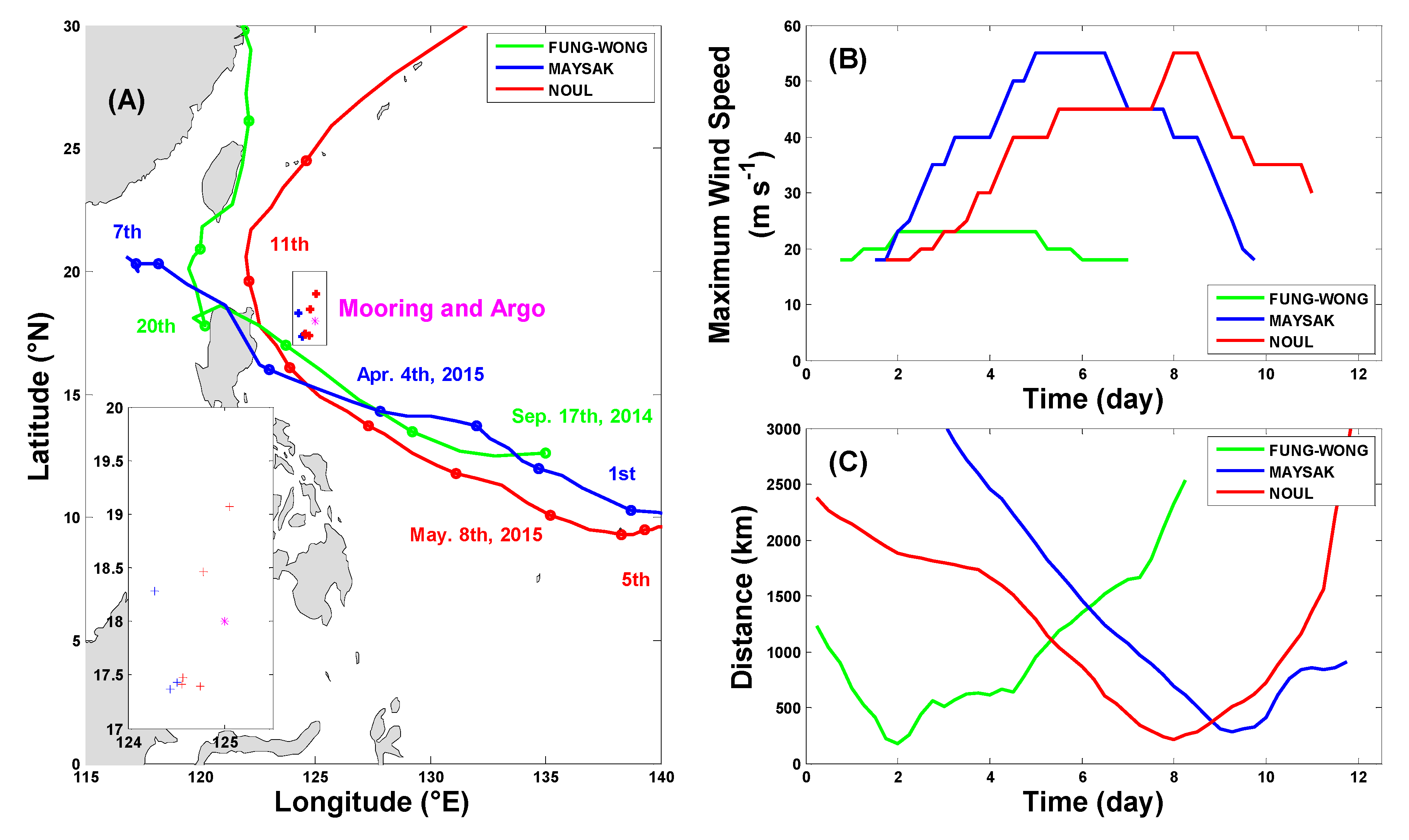
Three typhoons passed the mooring during the observation period, with three corresponding energetic NIO events being recorded. The tracks of the three typhoons were obtained from the Japan Meteorological Agency as shown in Figure 1A, and the temporal evolutions of the maximum wind speed and distances between the typhoons and the mooring are displayed in Figure 1C. The first typhoon, named Fung-Wong, formed on 17 September 2014 near 135.0° E and 12.6° N, and dissipated on 25 October 2014 near 138.5° E and 37.5° N. Fung-Wong was 177.1 km from the mooring on 17 September and passed southwest of it with a maximum sustained wind speed of 23 m s−1 and a radius (with an average wind velocity more than 15 m s−1, which was also used later) of 500 km. The mooring, which was deployed on 26 September 2014, captured part of the NIO induced by Fung-Wong.
The second typhoon was Maysak, which formed on 26 March 2015 near 159.9° E and 6.7° N, and was closest to the mooring on 5 April 2015. The maximum wind speed sustained was 18 m s−1. The closest the typhoon center got to the mooring was 285.9 km, which exceeded its radius of 150 km. The large distance between the typhoon center and the mooring, as well as the low maximum wind speed probably made the NIO event associated with Maysak less energetic than that associated with Fung-Wong.
The third typhoon, Noul, formed on 2 May 2015 near 144.1° E and 7.4° N, and dissipated as a tropical storm on 16 May 2015 at 178.1° E and 48.7° N. Noul was closest to the mooring on 10 May, and the smallest distance between its center and the mooring was 211.8 km. The maximum sustained wind speed was 55 m s−1 and the maximum wind speed radius was about 280 km.
Argo is a global array of about 3800 freely drifting buoys that measure temperature and salinity profiles in the top 2000 m of the oceans. It has been used in many studies on global changes and regional effects [38]. In this study, Argo data for a radius of 100 km from the typhoon centers as the storm passed were used. No Argo data were available during Fung-Wong, three Argo profiles were available during Maysak, and five profiles were available during Noul. The positions of the Argo buoys that provided the data are shown in Figure 1.
3. Theoretical Analysis
From the basic dynamics theory of oceanic internal waves, the dispersion relationship for a propagating inertial wave could be written as Equation (1) [1],
where (k, l, m) is a three-dimensional wave number, ω is the wave frequency, f is the inertial frequency and N is the buoyancy frequency.
The Boussinesq approximation was applied in the f plane, implying the change in frequency f with latitude could be neglected. This simplification is achievable for this single mooring position. The displacement of the mooring position is much smaller than the change of f with latitude.
The vertical group velocity Cgz can therefore be written as:
where the relationship between vertical group velocity Cgz and m can be calculated by:
where A = N2(k2 + l2) to simplify the equation.
The border limitations mean that velocity and pressure can be written as the product of the vertical mode item and the horizontal item, as shown in Equation (4).
where Ψ(z) is the vertical mode of velocity and pressure. U, V, W, and P are the horizontal structure of velocity and pressure. As the vertical velocity at the surface and seabed is zero. Thus, the boundary conditions are expressed as:
where H is the water depth. The solution of the vertical mode is shown in Equation (6) [39]. To solve the equation, we assume that the water body is of uniform stratification, which means that the Buoyancy frequency is constant. With this simplification, Ψ(z) can be solved in the following Equation (7).
Here n is the mode number, which is a positive integer, like n = 1, 2, 3. This means that Ψ(z) changes in the horizontal current direction as a function of depth. The larger is n in Equation (6), then Ψ(z) has more zero solutions under the same conditions. They have more times of horizontal current direction changes at the same times. Meanwhile, the vertical wave vector m = nπ/H so that the vertical wave number m is proportional to the number of modes n, m ∝ n.
In the case where the Buoyancy frequency N is not a constant, Ψ(z) will have different forms of solution, such as in Zervakis et al. in 1995 [40]. The good news is the conclusion that m and n are in a relatively increasing relationship and can still be obtained [40,41].
From Equations (3) and (6), it can be seen that the more the velocity changes with depth, the more NIKE propagates downward. The group velocity was downward; therefore, the vertical group velocity Cgz is less than zero. A larger vertical wave number m would make Cgz smaller. Considering that vertical wave number m is proportional to the number of modes n, a larger n will give a smaller Cgz. Even though we have no idea of velocity at full depth, the direction-changing times of the velocity at the known depth can also be used to describe the complexity of the velocity. The more times the vertical velocity changes with depth, the larger will be the n produced. Thus, if vertical velocity changed more times in the unit depth, a smaller Cgz would exist. This is similar to previous studies, such as [2,40,41]
To study the relationship between the vertical group velocity Cgz and the vertical stratification, Equation (7) can be derived from Equation (2). Based on these assumptions, the absolute group velocity (–Cgz) is an increasing function related to the buoyancy frequency N as below:
4. Results for Typhoon-Generated NIOs
4.1. Near-Inertial Responses
Frequency bands are selected to suit local NIO characteristics. For example, Shay et al. [42] used 0.8 f–1.2 f for the Gulf of Mexico, Chen et al. [43] used 0.85 f–1.15 f for the South China Sea, and Pallàs et al. [35] used 0.9 f–1.15 f for the Gulf of Mexico. In this study, the passband was based on 1/e (the reciprocal Euler’s number) of the power spectrum maximum for the average depth. This method prevented the main NIO signal information from being lost when the velocity spectrum was significant in a wider spectral band. The selected passband frequency for the NIOs was 0.7 f–1.2 f (see Figure 2).
The power spectra of the horizontal currents are at average depth (from 50 to 800 m), while the typhoons influencing the conditions (21 days) are shown in Figure 3. The inertial signal was the clearest signal during each event. Velocity spectra for the three NIO events are shown in Figure 2. The maximum spectral density of the first, second, and third NIOs were 0.172 m2 s−2 Hz−1 at 140 m, 0.049 m2 s−2 Hz−1 at 115 m, and 0.115 m2 s−2 Hz−1 at 145 m, respectively. The maximum inertial energy peaks were all deeper than 100 m, meaning that the most energetic NIOs did not appear at the surface. The peaks in the NIO frequency spectra were all clearly red-shifted and were all at 0.91 f (i.e., lower than the local inertial frequency f). The strongest red-shift was about 0.91 f and was between 100 and 300 m deep.
4.2. Near-Inertial Horizontal Current
The horizontal current time series was band-filtered (from 0.7 f to 1.2 f) to allow the near-inertial features to be analyzed. As mentioned earlier, the first typhoon was closest to the mooring location on 19 September 2014, seven days before the mooring was deployed. As shown in Figure 4, the maximum zonal velocity was 0.51 m s−1 and the maximum meridional velocity was 0.58 m s−1, both at 135 m deep. The second NIO event was the weakest of the three because the distance from the second typhoon’s center to the mooring site was further than for the other two typhoons, and its radius was smaller. The maximum zonal and meridional near-inertial velocities were 0.30 and 0.32 m s−1, respectively, both at a depth of 145 m. The third near-inertial event had a maximum zonal velocity of 0.47 m s−1 at 215 m deep and a maximum meridional velocity of 0.45 m s−1 at 175 m.
The directions of the horizontal currents changed four or five times between 40 and 800 m during the three NIO events. Pallàs et al. [35] observed near-inertial horizontal currents with two direction changes between the surface and depth of 1,400 m in the Gulf of Mexico. Meanwhile, Shay et al. [42] observed NIOs in the Gulf of Mexico by examining airborne expendable current profiles, and the horizontal current directions also changed twice between the surface and 800 m. Kim et al. [33], for their part, found that near-inertial horizontal current directions changed twice between the surface and 500 m in the northwest Pacific, nearly 2,000 km east of our mooring. All these researchers observed the baroclinic structure of the first near-inertial baroclinic mode, where surface horizontal currents are 180 degrees out of phase in respect to horizontal currents at depth. The horizontal currents changed more frequently in our observations than in those of our predecessors, implying that the NIOs at the mooring had higher modes and more complex vertical structures than those in the previous studies [33,35,39].
As shown in Figure 1, the first typhoon (FUNG-WONG) was closest to the Mooring, so it stimulated a strong near-inertial internal wave. The second typhoon (MAYSAK) had the smallest wind speed and the farthest distance, and the near-inertial internal wave excited was the smallest. Although the third typhoon (NOUL) was far away (similar to the second one), the intensity of the typhoon was large, so the intensity of the near-inertial internal wave was also relatively large, which is close to the first event.
4.3. Vertical Propagation of Near-Inertial Kinetic Energy
After the three typhoons passed, NIKE was concentrated in the upper 400 m of the water (Figure 5), where the density was 1.025 × 10³ kg m−3 (the average ocean-water density). NIKE below 400 m is not shown in this section because it was not strong enough. The black lines in Figure 5 indicate the maximum NIKE divided by e, to indicate the e-folding time. Inside the observation area, the maximum NIKE per unit mass (unit: kg, as in following) after the first typhoon was 163.64 J near depth of 135 m at 07:00 on 28 September 2014. The maximum NIKE per unit mass after the second typhoon was 51.83 J near depth of 130 m at 14:00 on 15 April 2015. The maximum NIKE per unit mass after the third typhoon was 113.60 J near depth of 195 m at 14:00 on 20 May 2015.
The outline in Figure 5 is the contour of the maxima NIKE divided by e. Because the first NIO was not the full NIO event, its e-folding time had to be estimated based on the second and third events. From the outline, the e-folding times for the second and third NIOs were 7 and 13 days, respectively. The mooring was deployed seven days after typhoon Fung-Wong had passed the mooring site. Meanwhile, the initial calculation time of the second NIO events is eight days after the typhoon coming, and the initial calculation time of the second NIO events is two days. So, for the first NIO events, the time between the occurrence of the first typhoon and the occurrence of first NIO takes the average of the second and third times. It is estimated that for the first NIO events, the initial calculation time is five days. So the e-folding time of the first NIO was estimated to be 16 days. Interestingly, all the NIKE maxima were deeper than 100 m rather than in the surface layer, consistent with the near-inertial currents.
From Figure 5, we can see that the estimated vertical group velocities of the first, second, and third NIOs were 11.9, 7.4, and 23.0 m d−1, respectively. The second typhoon gave a correspondingly weak NIO response, and the NIKE could barely propagate downward. The maximum NIKE for the third NIO was at 175 m deep. The group velocities were fairly small compared with those found in other studies (Table 1). This observed slow downward propagation was examined via a theoretical analysis in the previous section (based on Equations (3) and (6)).
4.4. Vertical Structure of the Buoyancy Frequency and Background Current during Typhoon-Generated NIOs
The cruise conductivity temperature depth (CTD) and ARGO data are combined in Figure 6. The N values for the said data were averaged inside an area of 150 km around the mooring location. The depth of N decreased sharply from 100 to 175 m during the first NIO (Figure 6A), based on the CTD data, and the maximum NIKE was 135 m deep. In the second NIO, N decreased sharply from 100 to 130 m (Figure 6B), and the maximum NIKE was at 127 m, based on the ARGO data. In the third NIO, N decreased sharply at three depths between 155 and 180 m (Figure 6C), and the maximum NIKE was at 175 m.
Figure 7 describes the mean flow characteristics at the mooring array. During the first NIO, the zonal current field was westward upper of approximately 600 meters, and the maximum westward velocity was 0.27 ms−1. The meridional current fields are all northward. The maximum northward velocity is 0.59 ms−1. The flow during the second NIO is southwestward for the first six days. Then it changed to northeastward afterwards. The maximum eastward velocity was 0.47 ms−1, and the maximum westward velocity was 0.33 ms−1. During the third NIO, the flow field direction remains in the southeast direction. The maximum eastward velocity was 0.76 ms−1, and the maximum westward velocity was 0.52 ms−1.
4.5. Vertical Structure of the Typhoon-Generated NIOs
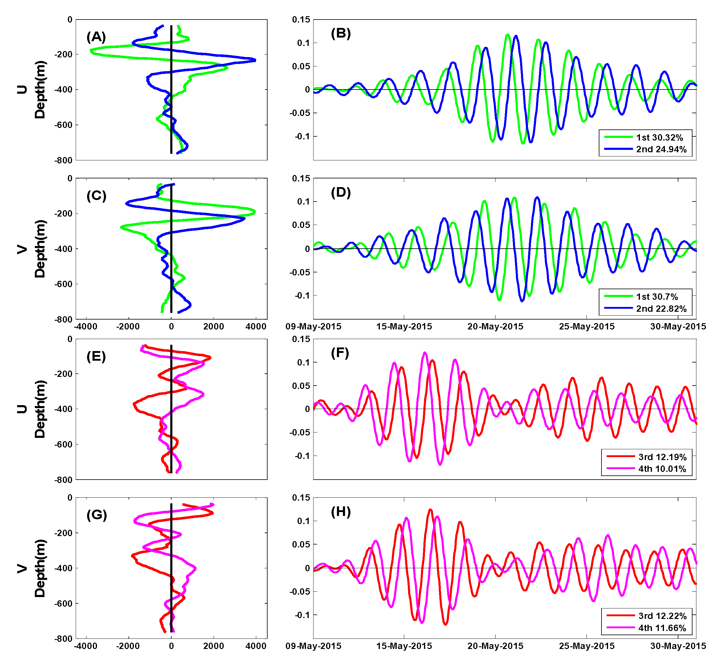
Bandpass filtering allows us to get the results of the near-inertial current. Meanwhile, in order to analyze the vertical structure of the near inertial current, empirical orthogonal function (EOF) analysis was used in this study. This method is widely used in the study of vertical structures of near inertial waves and internal tides, like Xu et al. in 2013 [44] and Yang et al. in 2015 [5]. For the first NIO (Figure 8), the first two modes dominated the near-inertial waves and contributed more than 80% of the total NIKE. The first mode contributed about 43.7% of the total, and the second mode about 39%. The vertical modes indicate that both components changed five times between the surface layer and depth of 800 m. The third and fourth modes contributed only 7.5% and 5.2%, respectively, of the total NIKE. The strongest signal of the first and second modes came at the same time as the strongest NIO signal. The strongest signal of the third and fourth modes was found earlier than the strongest NIO signal.
The second NIO event had only half the amplitude of the first (Figure 9). As for the NIKE pattern (Figure 5A), the first and second modes gained their maximum amplitudes on 15 April 2015 and changed four times over the observed depth range. The third mode’s maximum spatial amplitude occurred earlier than the maximum of the total NIO event, while the fourth mode’s maximum spatial amplitude occurred later than the maximum of the total NIO event. This indicates that the signals of these two modes may have been caused by something other than the typhoon. The average contributions of the first, second, third, and fourth modes to the total NIKE were 30.8%, 25.1%, 12.3%, and 10.1%, respectively.
The complete evolution of the third NIO was captured by the mooring (Figure 10). The amplitude trends in the time series for the first two modes were the same as for the total energy. The maximum amplitudes of the time series for the third and fourth modes were earlier than the maximum amplitude of the total energy. The first mode had five nodes and contributed 30.6% of the total NIKE; the second mode had four nodes and contributed 24.0% of the total NIKE; the third and the fourth modes contributed 12.2% and 10.2%, respectively, of the total NIKE; the third and fourth modes of the third NIO event contributed little to the total NIKE.
The EOF analysis can decompose the overall near-inertial current into different current modalities, giving us the spatial distribution and time series of each modal near-inertial current. Meanwhile, the time series of each modal near-inertial current has its own unique frequency. Although the frequency of each current is close to the inertial frequency, the frequency peaks are still different. The spectra of the time series were analyzed to allow the frequencies of the modes to be assessed (Figure 11). The most interesting finding was that the peak first and second mode frequencies for all three NIOs were red-shifted (i.e., were smaller than f) while the peak third and fourth mode frequencies were blue-shifted (bigger than f), except for the zonal velocity of the fourth mode for the first NIO. Taking the vertical structures of the NIOs into consideration, we found that the first and second modes followed a pattern of having four or five nodes, which means that the vertical structures of these two modes changed four or five times from a depth of 50 to 800 m.
The EOF results for the three NIO events exhibited many similarities. First, the contributions of the first two modes to the total NIKE were similar and around twice those of the third and fourth. Second, the time series and vertical modes of the first two modes were regular. The vertical modes changed four or five times along the observed depth, and the time series frequencies were <f, which is similar to the pattern for the total NIO signal. The third and fourth modes, in contrast, were not similar. We found that the typhoons mostly controlled the first and second modes of the NIO signals and that the third and fourth modes were similar to NIO signals that were not affected by the typhoons.
4.6. Vertical Structure of Non-Typhoon Period Data
Near-inertial currents, at times when they were uninfluenced by typhoons, were examined using the same methods to identify the different wave patterns at the times when they were influenced and not influenced by typhoons. The e-folding time was about 15 days, meaning that a time range of one month was used for the EOF analysis. The ADCP data were calculated month-by-month using the methods described above, with many similarities being discovered. Because the said data were available for almost 14 months, we used the EOF modes for January 2015 (Figure 12) and September 2015 (Figure 13) as examples.
5. Discussion
As mentioned earlier, the structures we found were more complex than those that have been found in previous studies, such as Pallàs et al. [35] in the Gulf of Mexico, Chen et al. [43] in the South China Sea, and Kim et al. [33] to the east of our mooring. This explains the much smaller Cgz in our study than in previous studies. Given the e-folding time and slow vertical group velocity, the typhoon-induced internal waves in this region were less likely to influence the deeper sea than was the case in previous studies. The observer may note from Figure 5 that the e-folding scales of the three NIOs we studied were less than 400 m. The NIKE weakened to 0.1 times the maximum more than 400 m depth, and the NIOs could only exert a clear influence at smaller than 400 m (Figure 5), which is much shallower than the 1,500 m found in the Gulf of Mexico [35].
As shown in Figure 5, the maximum NIKEs in the observation area for the first, second, and third NIOs were found at 135, 127, and 175 m, respectively. This mirrors many previous studies, in which none of the maximum NIKEs were at the surface [35]. Some researchers have explained this using a region termed inertial chimneys, which is created by anticyclonic eddies [45,46]. However, strong circulation and widely varying characteristics in our study area mean that anticyclonic eddies would not have persisted. The buoyancy frequency distribution should therefore be taken into consideration.
To study the relationship between energy transfer and water stratification, some simplifications are needed. We assumed that in one NIO event, although the wave number k was not determined, the change in wave numbers (k, l, m) could be neglected for downward energy transmission. As shown in Equation (2), the group velocity Cg is a function of the buoyancy frequency N when the wave number (k, l, m) is stable. The NIKE distribution can be simplified as a distribution of N (see Equation (7)).
Using Equation (7), we can calculate the downward group velocity (–Cgz) and the buoyancy frequency N in a monotonically increasing relationship. Here NIO can more easily be transmitted downward in an area with a larger N. In other words, NIKE will accumulate where N decreases sharply with depth. The maximum NIKE can be found at the depth at which Cg is large in the upper layer or small in the lower layer.
The most obvious feature of the NIOs influenced by typhoons is shown in Figure 8, Figure 9, and Figure 10. For the three NIO events the first mode explained greater than 30% of the variance and the second mode explained no smaller than 24%. The different modes did not make significantly different contributions during periods untroubled by typhoons. The amplitudes of the vertical structures were much stronger at less than 300 m deep than at deeper than 300 m when the typhoons were exerting their influences. The vertical distributions of the eastward and northward velocities alternated four or five times during this period. The amplitudes varied to be of lesser degree, and the vertical structures changed irregularly in periods unaffected by typhoons. The most interesting aspect was the time series when a typhoon was exerting its influence. The peak frequencies of the first two modes were smaller than f, and the frequencies of the third and fourth modes were bigger than f. The frequency of almost every mode in periods unaffected by typhoons was bigger than f, so the first and second modes may have been typhoon-induced signals in the cases when typhoons occurred.
The results of this study provide useful and intriguing insights into NIOs in the northwest Pacific. However, as shown in Equation (2), the vertical group velocity depends largely on the change of buoyancy frequency N, vertical wave number m, and horizontal wave numbers k and l. The complexity of the ocean means that wave numbers may change during the propagation process, weakening the correlation between Cg and N. Although Qi et al. presented a method for calculating the vertical wave number for a mooring [18], we could not obtain 4D data for the wave number. We are currently exploring the relationship between Cg and N using the marine model. Therefore, it still needs to be refined in future study.
6. Conclusions
Three energetic typhoon-generated NIO events were examined based on subsurface mooring observations lasting over 16 months (473 days) in the northwest Pacific Ocean. Compared to previous studies, a relatively wider band of the NIO energy concentrating at 0.7 f–1.2 f and stronger redshift of the NIO signals were reported in this study.
The maximum amplitudes of the observed near-inertial currents during three typhoon passages were 0.58, 0.32, and 0.47 m s−1, respectively, with current directions changing four or five times from the surface to a depth of 800 m. Group velocities of the first, second, and third NIO were 11.9, 7.4, and 23.0 m d−1, respectively, which were lower than those reported by previous studies. The e-folding times of the first, second, and third NIO events were 16, 7, and 13 days, respectively.
The EOF analysis indicated high mode vertical structures of the three NIO events, with energy mostly concentrating at the first two modes. Contributions from the first two modes were comparative and were more than twice larger than that from the third and fourth modes. Peak energy frequencies of the first two modes were less than f, but that of the third and fourth modes were mostly higher than f. Furthermore, non-typhoon-period NIO signals had frequencies more than f, suggesting a possibility that the third and fourth modes of the three NIO signals were not directly generated by the passages of typhoons.
Theoretical analyses demonstrated that the vertical group velocity of NIOs decreased with the increasing vertical wave numbers. The more times the velocity direction changes within a unit of length, the higher the vertical wave number will be, and the harder it will be to transmit energy downward. By considering the high mode vertical structure of the observed NIOs here, it can partially explain why the group velocity was relatively small in this study. However, it still needs to be refined in detail in future studies.
Author Contributions
Conceptualization, H.H. and F.Y.; Methodology, F.Y.; Software, F.N.; Validation, B.Y., S.G. and Y.Z.; Formal Analysis, H.H.; Investigation, F.Y.; Resources, F.Y.; Data Curation, H.H.; Writing-Original Draft Preparation, H.H.; Writing-Review & Editing, Y.Z.; Visualization, B.Y.; Supervision, Y.Z.; Project Administration, F.Y.; Funding Acquisition, F.Y.
Funding
This research is jointly supported by the National Key R&D Program of China (No. 2017YFC1403400 and 2016YFC1402003), the National Natural Science Foundation of China (No. U1406401, No. 41421005), and Global Change and Air Sea Interaction Project (No. GASI-02-PAC-STMSspr).
Acknowledgments
This research was jointly supported by the National Key R&D Program of China (No. 2017YFC1403400 and 2016YFC1402003), the National Natural Science Foundation of China (No. U1406401, No. 41421005), and Global Change and Air Sea Interaction Project (No. GASI-02-PAC-STMSspr). We also thank Qiang Ren and Chuanjie Wei for helping data collection.
Conflicts of Interest
The authors declare no conflict of interest.
References
- Garrett, C. What is the “near-inertial” band and why is it different from the rest of the internal wave spectrum? J. Phys. Oceanogr. 2001, 31, 962–971. [Google Scholar] [CrossRef]
- Alford, M.H.; MacKinnon, J.A.; Simmons, H.L.; Nash, J.D. Near-inertial internal gravity waves in the ocean. Annu. Rev. Mar. Sci. 2016, 8, 95–123. [Google Scholar] [CrossRef]
- Alford, M.H. Redistribution of energy available for ocean mixing by long-range propagation of internal waves. Nature 2003, 423, 159. [Google Scholar] [CrossRef]
- Guan, S.; Zhao, W.; Huthnance, J.; Tian, J.; Wang, J. Observed upper ocean response to typhoon Megi (2010) in the Northern South China Sea. J. Geophys. Res. Oceans 2014, 119, 3134–3157. [Google Scholar] [CrossRef] [Green Version]
- Yang, B.; Hou, Y.; Hu, P.; Liu, Z.; Liu, Y. Shallow ocean response to tropical cyclones observed on the continental shelf of the northwestern South China Sea. J. Geophys. Res. Oceans 2015, 120, 3817–3836. [Google Scholar] [CrossRef] [Green Version]
- Gregg, M.C. Diapycnal mixing in the thermocline: A review. J. Geophys. Res. Oceans 1987, 92, 5249–5286. [Google Scholar] [CrossRef]
- Price, J.F. Upper ocean response to a hurricane. J. Phys. Oceanogr. 1981, 11, 153–175. [Google Scholar] [CrossRef]
- Alford, M.H. Improved global maps and 54-year history of wind-work on ocean inertial motions. Geophys. Res. Lett. 2003, 30. [Google Scholar] [CrossRef] [Green Version]
- Fu, L.L. Observations and models of inertial waves in the deep ocean. Rev. Geophys. 1981, 19, 141–170. [Google Scholar] [CrossRef]
- Garrett, C.; Munk, W. Space-time scales of internal waves: A progress report. J. Geophys. Res. 1975, 80, 291–297. [Google Scholar] [CrossRef]
- Silverthorne, K.E.; Toole, J.M. Seasonal kinetic energy variability of near-inertial motions. J. Phys. Oceanogr. 2009, 39, 1035–1049. [Google Scholar] [CrossRef]
- Alford, M.H. Sustained, full-water-column observations of internal waves and mixing near Mendocino Escarpment. J. Phys. Oceanogr. 2010, 40, 2643–2660. [Google Scholar] [CrossRef]
- Jochum, M.; Briegleb, B.P.; Danabasoglu, G.; Large, W.G.; Norton, N.J.; Jayne, S.R.; Alford, M.H.; Bryan, F.O. The impact of oceanic near-inertial waves on climate. J. Clim. 2013, 26, 2833–2844. [Google Scholar] [CrossRef]
- Pollard, R.T.; Millard, R.C., Jr. Comparison between observed and simulated wind-generated inertial oscillations, Deep Sea Research and Oceanographic Abstracts. In Deep Sea Research and Oceanographic Abstracts; Elsevier: Amsterdam, The Netherlands, 1970; Volume 17, pp. 813–821. [Google Scholar]
- D’Asaro, E.A. The energy flux from the wind to near-inertial motions in the surface mixed layer. J. Phys. Oceanogr. 1985, 15, 1043–1059. [Google Scholar] [CrossRef]
- Sanford, T.B.; Price, J.F.; Girton, J.B. Upper-ocean response to Hurricane Frances (2004) observed by profiling EM-APEX floats. J. Phys. Oceanogr. 2011, 41, 1041–1056. [Google Scholar] [CrossRef]
- Rossby, C.G. On the mutual adjustment of pressure and velocity distributions in certain simple current systems. Mar. Res. 1938, 1, 239–263. [Google Scholar] [CrossRef]
- Qi, H.; De Szoeke, R.A.; Paulson, C.A.; Eriksen, C.C. The structure of near-inertial waves during ocean storms. J. Phys. Oceanogr. 1995, 25, 2853–2871. [Google Scholar] [CrossRef]
- Price, J.F. Internal wave wake of a moving storm. Part I. Scales, energy budget and observations. J. Phys. Oceanogr. 1983, 13, 949–965. [Google Scholar] [CrossRef]
- D’Asaro, E.A.; Sanford, T.B.; Niiler, P.P.; Terrill, E.J. Cold wake of hurricane Frances. Geophys. Res. Lett. 2007, 34. [Google Scholar] [CrossRef]
- Chang, S.W.; Anthes, R.A. Numerical simulations of the ocean’s nonlinear, baroclinic response to translating hurricanes. J. Phys. Oceanogr. 1978, 8, 468–480. [Google Scholar] [CrossRef]
- Chen, C.; Reid, R.O.; Nowlin, W.D., Jr. Near-inertial oscillations over the Texas-Louisiana shelf. J. Geophys. Res. Oceans 1996, 101, 3509–3524. [Google Scholar] [CrossRef]
- Teague, W.J.; Jarosz, E.; Wang, D.W.; Mitchell, D.A. Observed oceanic response over the upper continental slope and outer shelf during Hurricane Ivan. J. Phys. Oceanogr. 2007, 37, 2181–2206. [Google Scholar] [CrossRef]
- Jaimes, B.; Shay, L.K. Near-inertial wave wake of Hurricanes Katrina and Rita over mesoscale oceanic eddies. J. Phys. Oceanogr. 2010, 40, 1320–1337. [Google Scholar] [CrossRef]
- Leaman, K.D.; Sanford, T.B. Vertical energy propagation of inertial waves: A vector spectral analysis of velocity profiles. J. Geophys. Res. 1975, 80. [Google Scholar] [CrossRef]
- D’Asaro, E.A.; Perkins, H. A near-inertial internal wave spectrum for the Sargasso Sea in late summer. J. Phys. Oceanogr. 1984, 14, 489–505. [Google Scholar] [CrossRef]
- Pinkel, R. Doppler sonar observations of internal waves: The wavenumber-frequency spectrum. J. Phys. Oceanogr. 1984, 14, 1249–1270. [Google Scholar] [CrossRef]
- Sanford, T.B. Spatial structure of thermocline and abyssal internal waves in the Sargasso Sea. Deep Sea Res. Part II: Top. Stud. Oceanogr. 2013, 85, 195–209. [Google Scholar] [CrossRef]
- Munk, W.; Wunsch, C. Abyssal recipes II: Energetics of tidal and wind mixing. Deep Sea Res. Part I: Oceanogr. Res. Pap. 1998, 45, 1977–2010. [Google Scholar] [CrossRef]
- Alford, M.H.; Whitmont, M. Seasonal and spatial variability of near-inertial kinetic energy from historical moored velocity records. J. Phys. Oceanogr. 2007, 37, 2022–2037. [Google Scholar] [CrossRef]
- Morozov, E.G.; Velarde, M.G. Inertial oscillations as deep ocean response to hurricanes. J. Oceanogr. 2008, 64, 495. [Google Scholar] [CrossRef]
- Alford, M.H.; Cronin, M.F.; Klymak, J.M. Annual cycle and depth penetration of wind-generated near-inertial internal waves at Ocean Station Papa in the northeast Pacific. J. Phys. Oceanogr. 2012, 42, 889–909. [Google Scholar] [CrossRef]
- Kim, E.; Jeon, D.; Jang, C.J.; Park, J.H. Typhoon Rammasun-Induced Near-Inertial Oscillations Observed in the Tropical Northwestern Pacific Ocean. Terr. Atmos. Ocean. Sci. 2013, 24, 761–772. [Google Scholar] [CrossRef]
- Yang, B.; Hou, Y.; Hu, P. Observed near-inertial waves in the wake of Typhoon Hagupit in the northern South China Sea. Chin. J. Oceanol. Limnol. 2015, 33, 1265–1278. [Google Scholar] [CrossRef]
- Pallàs-Sanz, E.; Candela, J.; Sheinbaum, J.; Ochoa, J.; Jouanno, J. Trapping of the near-inertial wave wakes of two consecutive hurricanes in the Loop Current. J. Geophys. Res. Oceans 2016, 121, 7431–7454. [Google Scholar] [CrossRef]
- Qu, T.; Kagimoto, T.; Yamagata, T. A subsurface countercurrent along the east coast of Luzon. Deep Sea Res. Part I: Oceanogr. Res. Pap. 1997, 44, 413–423. [Google Scholar] [CrossRef]
- Hu, D.; Hu, S.; Wu, L.; Li, L.; Zhang, L.; Diao, X.; Chen, Z.; Li, Y.; Wang, F.; Yuan, D. Direct measurements of the Luzon Undercurrent. J. Phys. Oceanogr. 2013, 43, 1417–1425. [Google Scholar] [CrossRef]
- Whalen, C.B.; Talley, L.D.; MacKinnon, J.A. Spatial and temporal variability of global ocean mixing inferred from Argo profiles. Geophys. Res. Lett. 2012, 39, 1–6. [Google Scholar] [CrossRef]
- Fang, X.; Du, T. Fundamentals of Oceanic Internal Waves and Internal Waves in the China Seas, 1st ed.; China Ocean University Press: Qingdao, China, 2005; pp. 27–31. (In Chinese) [Google Scholar]
- Zervakis, V.; Levine, M.D. Near-inertial energy propagation from the mixed layer: Theoretical considerations. J. Phys. Oceanogr. 1995, 25, 2872–2889. [Google Scholar] [CrossRef]
- Shay, L.K.; Chang, S.W. Free surface effects on the near-inertial ocean current response to a hurricane: A revisit. J. Phys. Oceanogr. 1997, 27, 23–39. [Google Scholar] [CrossRef]
- Shay, L.K.; Mariano, A.J.; Jacob, S.D.; Ryan, E.H. Mean and near-inertial ocean current response to Hurricane Gilbert. J. Phys. Oceanogr. 1998, 28, 858–889. [Google Scholar] [CrossRef]
- Chen, G.; Xue, H.; Wang, D.; Xie, Q. Observed near-inertial kinetic energy in the northwestern South China Sea. J. Geophys. Res. Oceans 2013, 118, 4965–4977. [Google Scholar] [CrossRef] [Green Version]
- Xu, Z.; Yin, B.; Hou, Y.; Xu, Y. Variability of internal tides and near-inertial waves on the continental slope of the northwestern South China Sea. J. Geophys. Res. Oceans 2013, 118, 197–211. [Google Scholar] [CrossRef] [Green Version]
- Lee, D.K.; Niiler, P.P. The inertial chimney: The near-inertial energy drainage from the ocean surface to the deep layer. J. Geophys. Res. Oceans 1998, 103, 7579–7591. [Google Scholar] [CrossRef] [Green Version]
- Young, W.R.; Jelloul, M.B. Propagation of near-inertial oscillations through a geostrophic flow. J. Mar. Res. 1997, 55, 735–766. [Google Scholar] [CrossRef]
Figure 1.
(A) Best tracks of typhoon Fung-Wong (No. 16) in 2014, typhoon Maysak (No. 4) in 2015, and typhoon Noul (No. 6) in 2015. The magenta asterisk indicates the location of the mooring, and the plus signs are the locations of the Argo buoys. The horizontal axis of (A) is longitude with the unit °E. The vertical axis is latitude with the unit °N. Locations of the Argo profiles were labeled with the different colors corresponding to different typhoon passages. (B) Maximum wind speed over time from when each typhoon was generated. The horizontal axis of (B) is time with the unit day. The vertical axis is maximum wind speed with the unit ms−1. (C) Distance between each typhoon and the mooring over time from when each typhoon was generated. The horizontal axis of (C) is time with the unit day. The vertical axis is distance with the unit km. All these three figures in Figure 1 have the same legend.

Figure 2.
The power spectra of the first near-inertial oscillation (NIO) event is shown in (A,D). The second is shown in (B,E). The third is shown in (C,F). The horizontal axis of the figure is frequency with the unit cpd. The vertical axis is water depth with the unit m. Power spectra of the (A–C) eastward and (D–F) northward components of the horizontal currents at 40–800 m deep for the three NIOs. The dashed lines indicate local frequencies f, 0.7 f, and 1.2 f. Note that the different color-bars represent the three typhoon events.

Figure 3.
Average power spectra for all the depths (from 50 to 800 m) velocities U = √(u2 + v2) at the mooring. The horizontal axis of the figure is the frequency with the unit cpd. The vertical axis is spectral density with the unit m2 s−2 cpd−1. The three different lines are the average power spectra of velocity after the three typhoons (Fung-Wong, Maysak, and Noul). The dotted lines indicate the local inertial frequency f, the frequency of the k1 tide, and the frequency of the m2 tide. This figure has the same legend as Figure 1.

Figure 4.
Time evolution of the cross-track component of the band-pass filtered (σ ∈ [0.7, 1.2] f) (A,C,E) eastward and (B,D,F) northward ocean currents (m s-1) at 40–800 m deep. The first near inertial current is shown in (A,B). The second is shown in (C,D). The third is shown in (E,F). The horizontal axis of the figure is time. The vertical axis is the water depth with the unit m. The black circles indicate the times the typhoons were closest to the mooring. Note that the different color-bars are for the three typhoon events.

Figure 5.
Time evolution of the band-pass (σ ∈ [0.7, 1.2] f) filtered near-inertial kinetic energy (NIKE) (in J). The horizontal axis of the figure is time. The vertical axis is the water depth with the unit m. The thick black lines are 1/e of the maxima NIKE. The black circles indicate the times the typhoons were closest to the mooring. NIKE below 400 m was too weak and not shown in this figure. For the three pictures to be presentable, the three colorbars are different.

Figure 6.
Regional average buoyancy frequency N calculated from the ARGO profiles (blue lines) and cruise conductivity temperature depth (CTD) profile (green line) during (A) the first NIO (in September 2014), (B) the second NIO (in April 2015), and (C) the third NIO (in May 2015). The horizontal axis of the figure is the Buoyancy frequency with the unit cpd. The vertical axis is water depth with the unit m. The red circle is the maximum NIKE depth. The selected sea area for the second and third NIOs was 100 km around the mooring location. No ARGO data were available for within 100 km of the mooring for the first NIO.

Figure 7.
Time evolution of the cross-track component of the low-pass filtered (σ smaller than 1/72 h−1) (A,C,E) eastward and (B,D,F) northward ocean currents (m s−1) at 40–800 m deep. The background current is shown in (A,B). The second is shown in (C,D). The third is shown in (E,F). The horizontal axis of the figure is time. The vertical axis is the water depth with the unit m. The black circles indicate the times the typhoons were closest to the mooring.

Figure 8.
Vertical profiles of the (A,E) eastward and (C,G) northward components of the near-inertial current and the corresponding (B,F) eastward and (D,H) northward time series by empirical orthogonal function (EOF) analysis. The first and second modes are shown in (A–D). Meanwhile, the third and fourth modes are shown in (E–H). The NIO event occurred in September 2014.

Figure 9.
As for Figure 8 but for the NIO event in April 2015.
Figure 9.
As for Figure 8 but for the NIO event in April 2015.

Figure 10.
As for Figure 8 but for the NIO event in May 2015.
Figure 10.
As for Figure 8 but for the NIO event in May 2015.

Figure 11.
Power spectra of the (A,C,E) eastward and (B,D,F) northward time series of the near-inertial currents in the three NIOs by EOF analyses results. The power spectra of the first NIO event is shown in (A,B). The second is shown in (C,D). The third is shown in (E,F). The horizontal axis of the figure is the relative frequency of the Coriolis frequency f. The vertical axis is spectral density with the unit m2s−2cpd−1. Each picture has the time series result of the first four modes by EOF analyses.

Figure 12.
Vertical profiles of the (A,E) eastward and (C,G) northward components of the near-inertial current and the corresponding (B,F) eastward and (D,H) northward time series by empirical orthogonal function (EOF) analysis. The first and second modes are shown in (A–D). Meanwhile, the third and fourth modes are shown in (E–H). Power spectra of the (I) eastward and (J) northward time series of the near-inertial currents in the three NIOs by EOF analyses result. The horizontal axis of the figure is the relative frequency of the Coriolis frequency f. The vertical axis is spectral density with the unit m2 s−2 cpd−1. (I,J) have the time series results of the first four modes by EOF analyses. The NIO signal occurred in January 2015.

Figure 13.
As for Figure 10 but the NIO signal occurred in September 2015.
Figure 13.
As for Figure 10 but the NIO signal occurred in September 2015.


Table 1.
Summary of vertical group velocity (Cg) values found in previous studies.
| Reference | Cg (m d−1) | Method |
|---|---|---|
| Price, 1983 [19] | 100 | MODEL |
| Qi et al., 1995 [18] | 7–39 FASTEST* 4–20 SLOWEST* | CURRENT METER |
| Kim et al., 2013 [33] | 39.7 | ADCP |
| Yang et al., 2015 [5] | 240 | ADCP |
| Yang et al., 2015 [34] | 233 | ADCP |
| Pallàs et al., 2016 [35] | 56 ± 7 | ADCP |
Note that: ADCP means acoustic Doppler current profilers.
© 2018 by the authors. Licensee MDPI, Basel, Switzerland. This article is an open access article distributed under the terms and conditions of the Creative Commons Attribution (CC BY) license (http://creativecommons.org/licenses/by/4.0/).
Share and Cite
MDPI and ACS Style
Hou, H.; Yu, F.; Nan, F.; Yang, B.; Guan, S.; Zhang, Y. Observation of Near-Inertial Oscillations Induced by Energy Transformation during Typhoons. Energies 2019, 12, 99. https://doi.org/10.3390/en12010099
AMA Style
Hou H, Yu F, Nan F, Yang B, Guan S, Zhang Y. Observation of Near-Inertial Oscillations Induced by Energy Transformation during Typhoons. Energies. 2019; 12(1):99. https://doi.org/10.3390/en12010099
Chicago/Turabian StyleHou, Huaqian, Fei Yu, Feng Nan, Bing Yang, Shoude Guan, and Yuanzhi Zhang. 2019. "Observation of Near-Inertial Oscillations Induced by Energy Transformation during Typhoons" Energies 12, no. 1: 99. https://doi.org/10.3390/en12010099
Note that from the first issue of 2016, this journal uses article numbers instead of page numbers. See further details here.