A New Method and Application of Full 3D Numerical Simulation for Hydraulic Fracturing Horizontal Fracture


Abstract
:1. Introduction
2. Mathematical Physics Equation
2.1. Elastic Rock Mechanics Equation
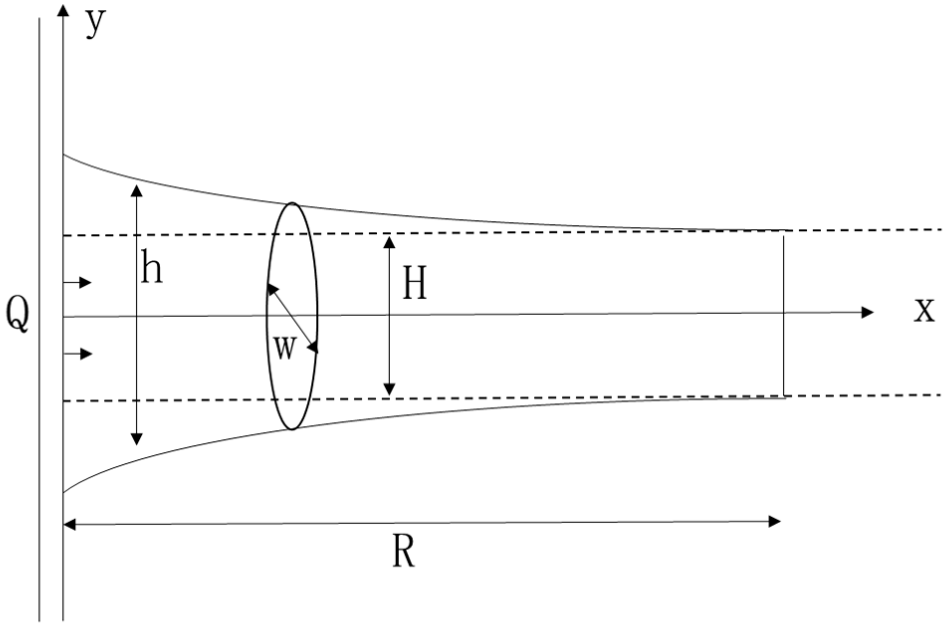
2.2. Material Flow Continuity Equation
3. Galerkin Finite Element Method and Equation Solution
3.1. Galerkin Finite Element Method
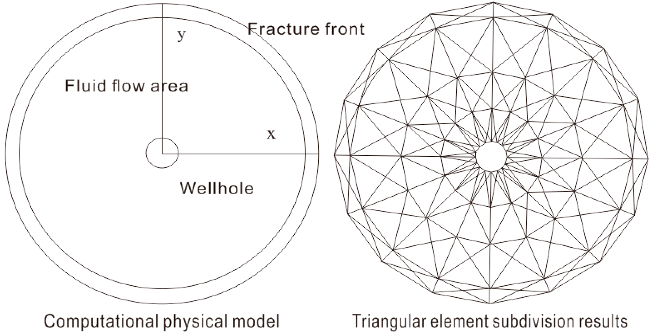
3.2. Three Node Triangular Isoparametric Element
3.3. The Solution of Integral Equation
3.4. Picard Iteration Method
3.5. Fracture Extension Judgement
4. Applications
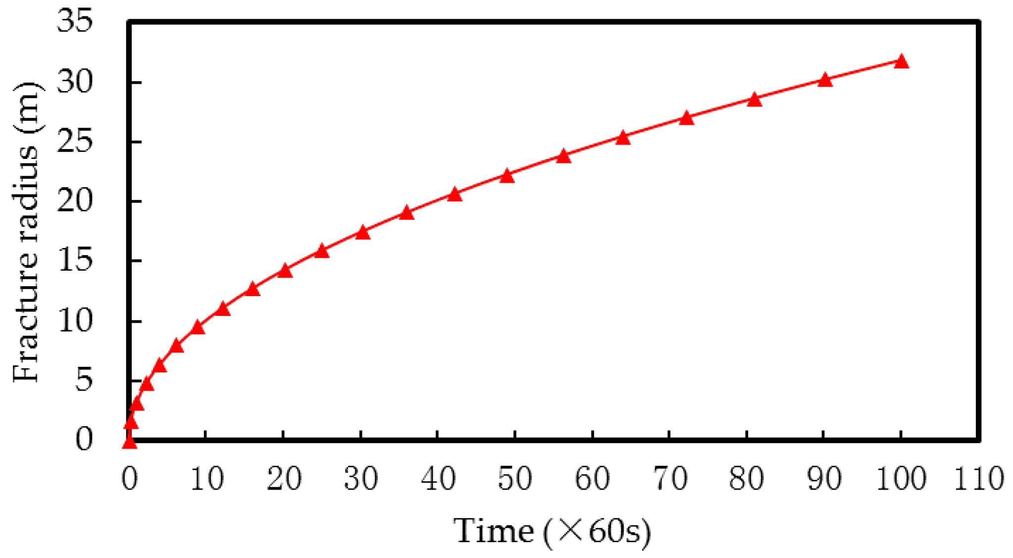
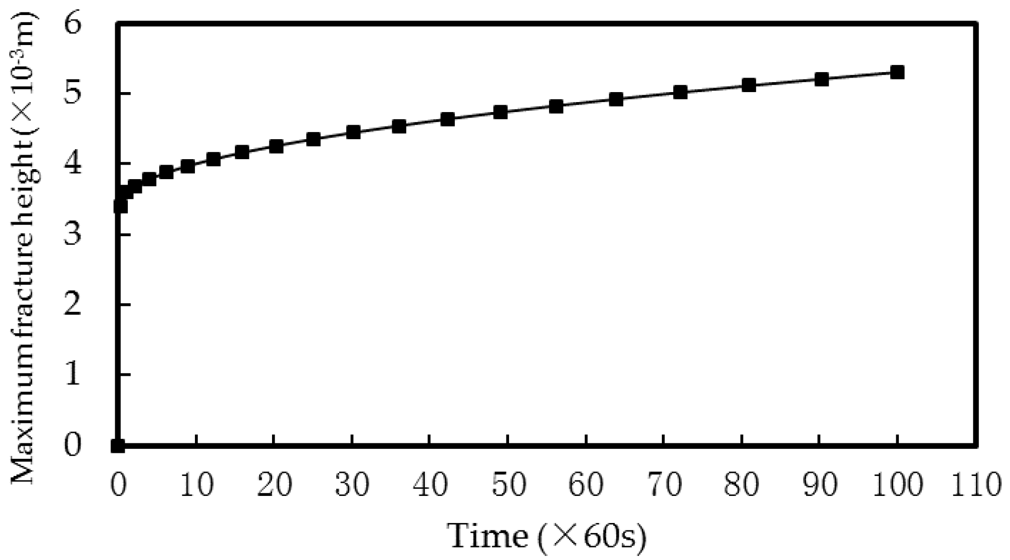
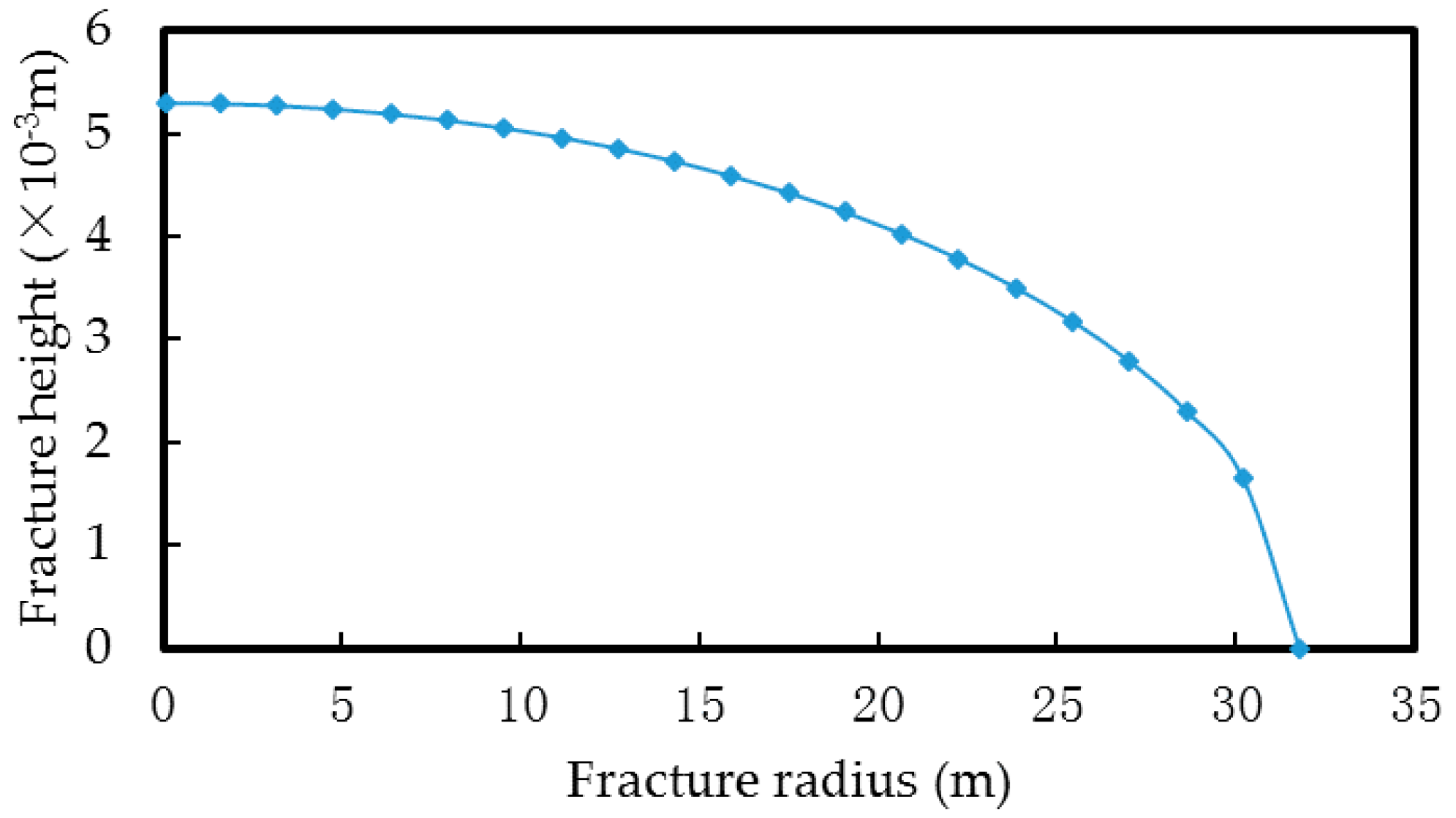
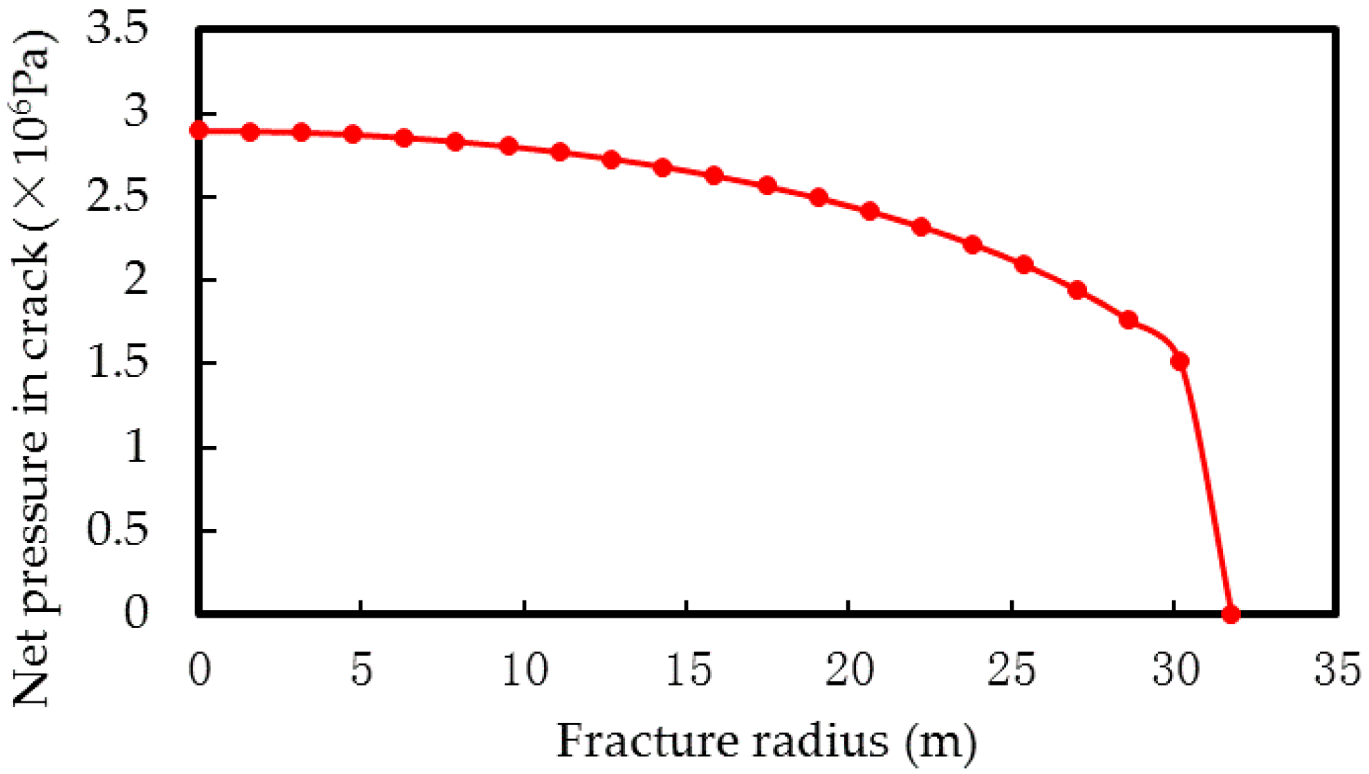
4.1. Example Analysis
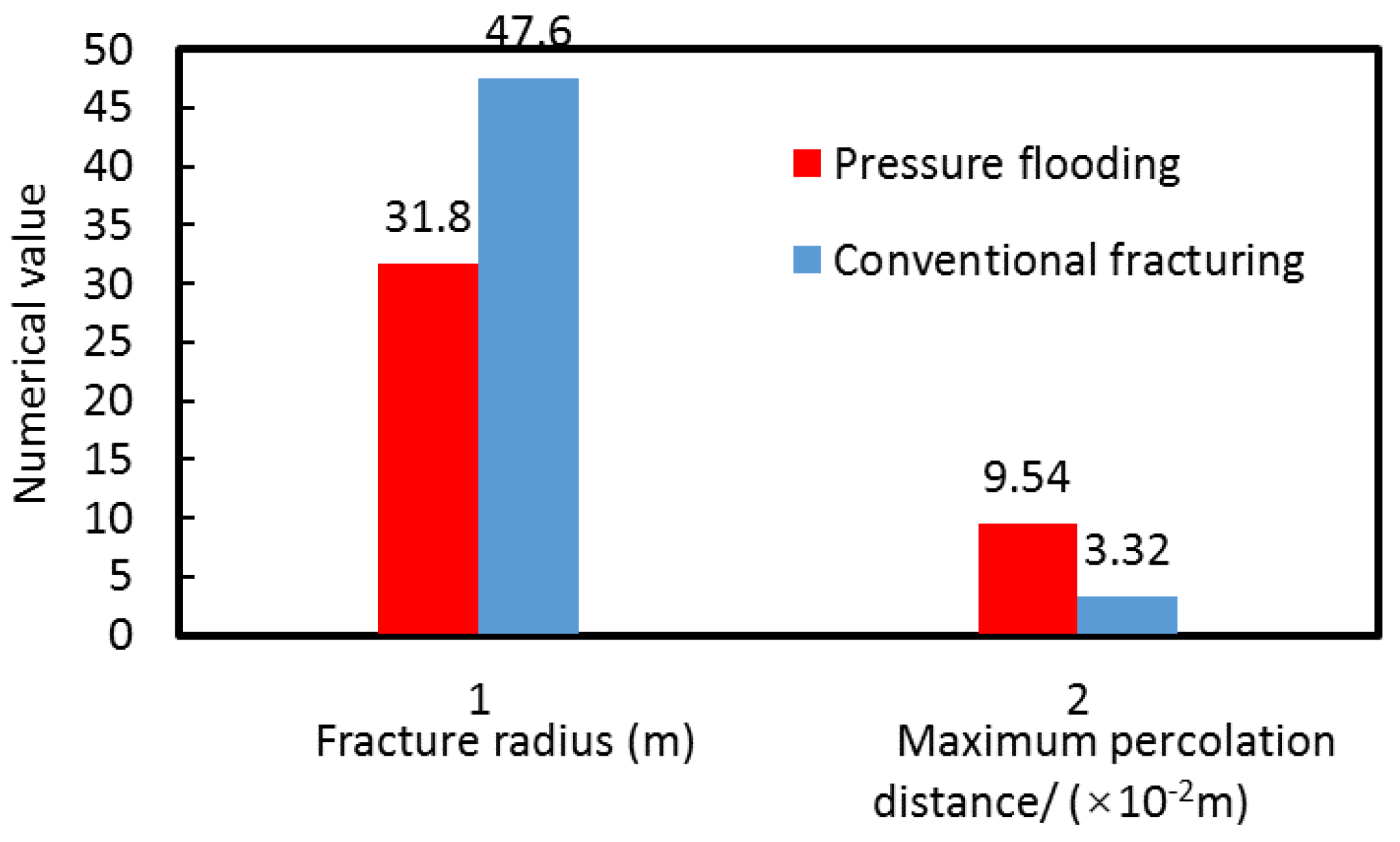
4.2. Factor Analysis
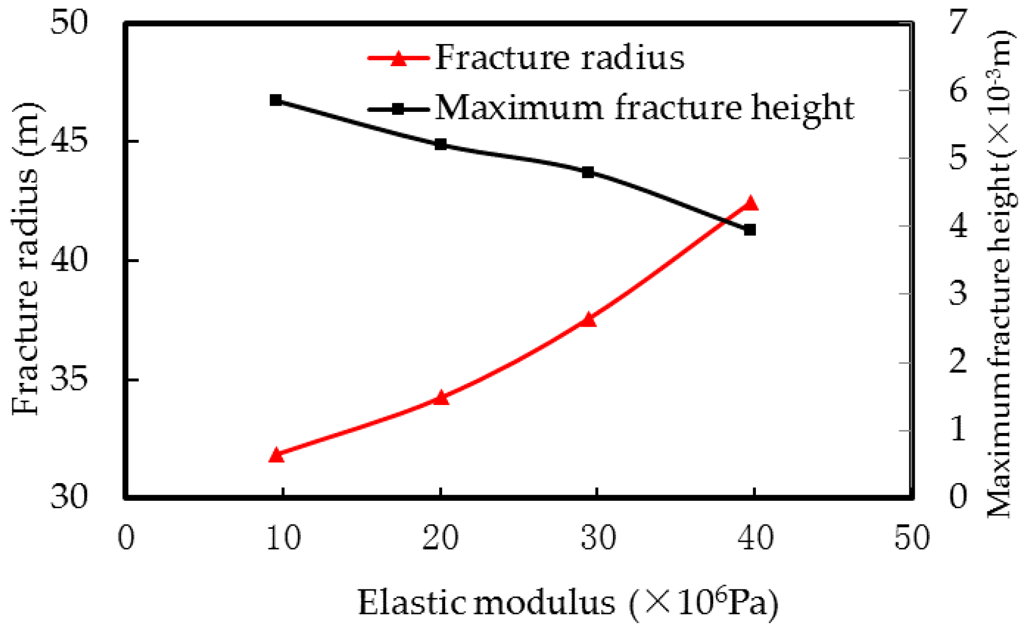
4.2.1. Rock Elastic Modulus
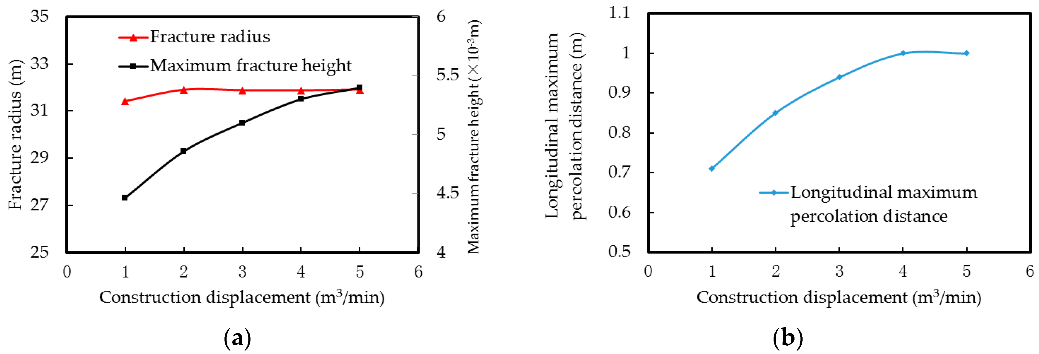
4.2.2. Construction Displacement
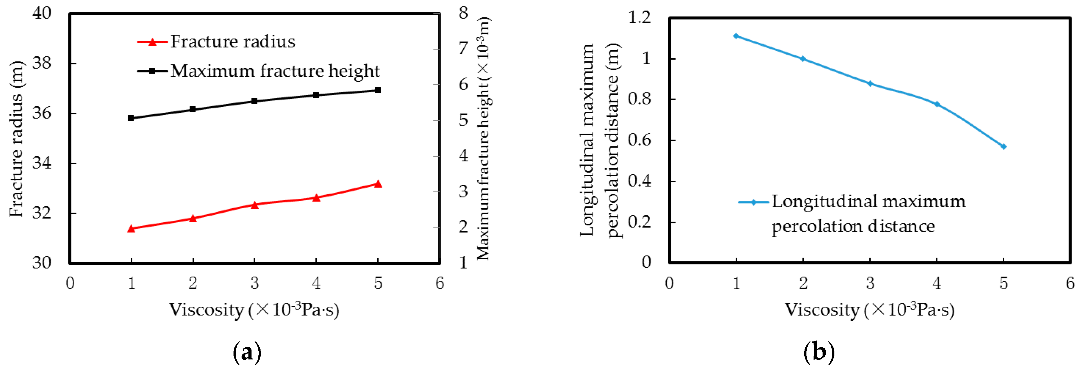
4.2.3. Viscosity of Fracturing Fluid
5. Results and Discussion
Author Contributions
Funding
Conflicts of Interest
References
- Perkins, T.K.; Kern, L.R. Widths of Hydraulic Fractures. J. Pet. Technol. 1961, 13, 937–949. [Google Scholar] [CrossRef]
- Geertsma, J.; de Klerk, F. A rapid method of predicting width and extent of hydraulically induced fractures. J. Petrol. Technol. 1969, 21, 1571–1581. [Google Scholar] [CrossRef]
- Bouteca, M.J. Hydraulic Fracturing Model Based on a Three-Dimensional Closed Form: Tests and Analysis of Fracture Geometry and Containment. SPE Prod. Eng. 1988, 3, 445–454. [Google Scholar] [CrossRef]
- Chen, M.; Jin, Y.; Zhang, G.Q. Petroleum Engineering Rock Mechanics; Science Press: Beijing, China, 2008. [Google Scholar]
- Rubin, M.B. On Fluid Leak-Off during Propagation of a Vertical Hydraulic Fracture; Paper SPE 10556-MS; Society of Petroleum Engineers: Richardson, TX, USA, 1981. [Google Scholar]
- Gurevich, A.E.; Chilingarian, G.V. Petroleum related rock mechanics: Erling Fjær, Rune M. Holt, Per Horstrud Arne M. Raaen and Rasmus Risnes. Developments in Petroleum Science, 33, 1992. Elsevier, Amsterdam, 338 pp. $110.50, ISBN 0-444-88913-2. J. Pet. Sci. Eng. 1993, 9, 352. [Google Scholar] [CrossRef]
- Adachi, J.; Siebrits, E.; Peirce, A.; Desroches, J. Computer simulation of hydraulic fractures. Int. J. Rock Mech. Min. Sci. 2007, 44, 739–757. [Google Scholar] [CrossRef]
- Cui, S.X. Ten years’ experience of in-situ stress hydrofracturing in tunnel construction in Korea. J. Rock Mech. Eng. 2007, 26, 2200–2206. [Google Scholar]
- Palmer, I.D. Three-Dimensional Hydraulic Fracture Propagation in the Presence of Stress Variations. Soc. Pet. Eng. J. 1983, 23, 870–878. [Google Scholar] [CrossRef]
- Palmer, I.D.; Carroll, H.B., Jr. Numerical solution for Height and Elongated Hydraulic Fractures. In Proceedings of the SPE/DOE Low Permeability Gas Reservoirs Symposium, Denver, CO, USA, 14–16 March 1983. Paper SPE/DOE 11627. [Google Scholar]
- Wang, H.X. Principle of Hydraulic Fracturing; Petroleum Industry Press: Beijing, China, 1987; pp. 56–69. [Google Scholar]
- Chen, S. Study on Influence Factors of Hydraulic Fracturing Propagation. Ph.D Thesis, Xi’an University of Technology, Xi’an, China, 2018; pp. 78–81. [Google Scholar]
- Zhang, B.; Li, X.; Wang, Y.; Wu, Y.F.; Li, G.Z. Research status and Prospect of hydraulic fracturing simulation technology for oil and gas reservoirs. J. Eng. Geol. 2015, 23, 301–310. [Google Scholar]
- Shen, Y.H.; Ge, H.K.; Cheng, Y.Y.; Xia, Y.M.; Li, N.; Yang, L. New method for numerical solution of quasi-three-dimensional hydraulic fracturing model. Sci. Technol. Eng. 2014, 14, 219–223. [Google Scholar]
- Xue, B.; Zhang, G.M.; Wu, H.A.; Wang, X.X. Three-dimensional numerical simulation of oil well hydraulic fracturing. J. China Univ. Sci. Technol. 2008, 11, 1322–1325, 1347. [Google Scholar]
- Qiao, J.T.; Zhang, R.J.; Yao, F.; Jiang, T. Two-dimensional temperature field analysis of hydraulic fracturing. J. Tongji Univ. (Nat. Sci. Ed.) 2000, 4, 434–437. [Google Scholar]
- Wu, J.Z.; Qu, D.B.; Meng, X.J. Study on Numerical Simulation of geometric shape of hydraulic fracturing fracture. J. Daqing Pet. Inst. 1988, 4, 30–36. [Google Scholar]
- Zhang, P.; Zhao, J.Z.; Guo, D.L.; Chen, W.B.; Tian, J.D. Three-dimensional numerical simulation of hydraulic fracturing fracture extension. Pet. Drill. Prod. Technol. 1997, 3, 53–59, 69–108. [Google Scholar]
- Wang, H.X.; Zhang, S.C. Numerical Calculation Method of Hydraulic Fracturing Design[M]; Petroleum Industry Press: Beijing, China, 1998; pp. 148–190. [Google Scholar]
- Kossecka, E. Defects as surface distributions of double forces. Arch. Mech. 1971, 23, 481–494. [Google Scholar]
- Gu, H.; Yew, C.H. Finite element solution of a boundary integral equation for mode I embedded three-dimensional fractures. Int. J. Numer. Methods Eng. 1988, 26, 1525–1540. [Google Scholar] [CrossRef]
- Ching, H.Y. Mechanics of Hydraulic Fracturing; Gulf Professional Publishing: Houston, TX, USA, 1997; pp. 30–60. [Google Scholar]
- Meyer, B.R. Design Formulae for 2-D and 3-D Vertical Hydraulic Fractures: Model Comparison and Parametric Studies. In Proceedings of the SPE Unconventional Gas Technology Symposium, Louisville, KY, USA, 18–21 May 1986. [Google Scholar]
- Wang, H.Z. Numerical Simulation Study of “Intra Layer Explosion”. Ph.D Thesis, Daqing Petroleum Institute, Daqing, China, 2009; pp. 11–13. [Google Scholar]
- Zhou, Z.J. Theory and Application of Fluid-solid Coupled Percolation in Low Permeability Reservoirs. Ph.D. Thesis, Daqing Petroleum Institute, Daqing, China, 2003; pp. 76–80. [Google Scholar]
- Liu, Y. Finite Element Analysis and Application[M]; China Electric Power Press: Beijing, China, 2008; p. 42. [Google Scholar]
- Abou-Sayed, A.S.; Clifton, R.J.; Dougherty, R.L.; Morales, R.H. Evaluation of the Influence of In-Situ Reservoir Conditions on the Geometry of Hydraulic Fractures Using a 3-D Simulator: Part 2-Case Studies. In Proceedings of the SPE Unconventional Gas Recovery Symposium, Pittsburgh, PA, USA, 13–15 May 1984. [Google Scholar]
- Ioakimidis, N.I. Exact expression for a two-dimensional finite-part integral appearing during the numerical solution of fracture problems in three-dimensional elasticity. Int. J. Numer. Methods Biomed. Eng. 2010, 1, 183–189. [Google Scholar]
- Clifton, R.; Abou-Sayed, A. A variational approach to the prediction of the three–dimensional geometry hydraulic fractures. In Proceedings of the SPE/DOE Low Permeability Gas Reservoirs Symposium, Denver, CO, USA, 27–29 May 1981. [Google Scholar]
- Sneddon, I.N. The Distribution of Stress in the Neighbourhood of a Fracture in an Elastic Solid. Proc. R. Soc. Lond. A 1946, 187, 229–260. [Google Scholar]
- Clifton, R.J.; Wang, J.J. Multiple Fluids, Proppant Transport, and Thermal Effects in Three-Dimensional Simulation of Hydraulic Fracturing. In Proceedings of the SPE Annual Technical Conference and Exhibition, Houston, TX, USA, 2–5 October 1988. [Google Scholar]
- Mastrojannis, E.N.; Keer, L.M.; Mura, T. Growth of planar fractures induced by hydraulic fracturing. Int. J. Numer. Methods Eng. 1980, 15, 41–54. [Google Scholar] [CrossRef]
- Pan, H.; Lu, X.G.; Xie, K.; Wang, K.X. The effect of fracturing fluid filtration on oil enhancement and its mechanism. Oilfield Chem. 2017, 34, 245–249. [Google Scholar]


| Model Parameter | Numerical Value | Reference Range |
|---|---|---|
| Reservoir elastic modulus/Pa | 12 × 109 | 10 × 109~40 × 109 |
| Poisson’s ratio of interlayer | 0.26 | 0.24~0.26 |
| Vertical stress/Pa | 23.2 × 10⁶ | 22 × 106~24 × 106 |
| Construction displacement/(m3/min) | 4.5 | 4~5 |
| Comprehensive filtration coefficient of conventional fracturing/() | 1 × 10‒4 | 0.01 × 10⁻⁴~1 × 10⁻⁴ |
| Comprehensive filtration coefficient of pressure drive technology/() | 10 × 10−4 | 10 × 10−4~100 × 10−4 |
| Viscosity of fracturing fluid/P·s | 2 × 10⁻³ | 1 × 10⁻³~5 × 10⁻³ |
| Viscosity of conventional fracturing fluids/P·s | 25 × 10−3 | 10 × 10−3~50 × 10−3 |
| Construction fluid volume/m3 | 450 | 100~1000 |
| Construction time/s | 6000 | 1500~15,000 |
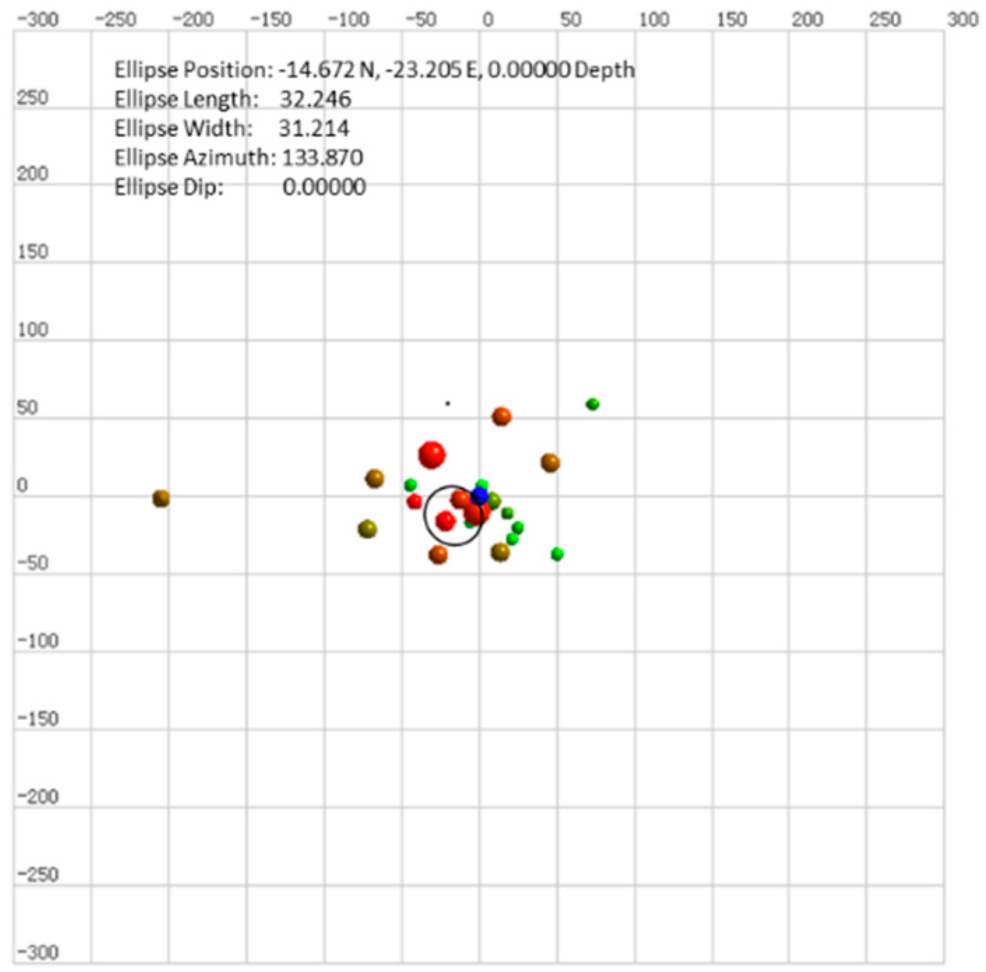
| Fracturing Horizon | Fracture Network Length (m) | Fracture Network Width (m) | Orientation of Fracture Network (°) | Number of Microseismic Events (number) |
|---|---|---|---|---|
| PI111~112 | 32.246 | 31.214 | 133.870 | 23 |
© 2018 by the authors. Licensee MDPI, Basel, Switzerland. This article is an open access article distributed under the terms and conditions of the Creative Commons Attribution (CC BY) license (http://creativecommons.org/licenses/by/4.0/).
Share and Cite
Xu, B.; Liu, Y.; Wang, Y.; Yang, G.; Yu, Q.; Wang, F. A New Method and Application of Full 3D Numerical Simulation for Hydraulic Fracturing Horizontal Fracture. Energies 2019, 12, 48. https://doi.org/10.3390/en12010048
Xu B, Liu Y, Wang Y, Yang G, Yu Q, Wang F. A New Method and Application of Full 3D Numerical Simulation for Hydraulic Fracturing Horizontal Fracture. Energies. 2019; 12(1):48. https://doi.org/10.3390/en12010048
Chicago/Turabian StyleXu, Bing, Yikun Liu, Yumei Wang, Guang Yang, Qiannan Yu, and Fengjiao Wang. 2019. "A New Method and Application of Full 3D Numerical Simulation for Hydraulic Fracturing Horizontal Fracture" Energies 12, no. 1: 48. https://doi.org/10.3390/en12010048
APA StyleXu, B., Liu, Y., Wang, Y., Yang, G., Yu, Q., & Wang, F. (2019). A New Method and Application of Full 3D Numerical Simulation for Hydraulic Fracturing Horizontal Fracture. Energies, 12(1), 48. https://doi.org/10.3390/en12010048