Adaptive Fuzzy Droop Control for Optimized Power Sharing in an Islanded Microgrid

Abstract

With the serious environment pollution and power crisis, the increasing of renewable energy resource (RES) becomes a new tendency. However, the high proportion of RES may affect the stability of the system when using the conventional droop control with a fixed droop coefficient. In order to prevent the power overloading/curtailment, this paper proposes an adaptive fuzzy droop control (AFDC) scheme with a P-f droop coefficient adjustment to achieve an optimized power sharing. The droop coefficient is adjusted considering the power fluctuation of RES units and the relationship of power generation and demand, which can realize the stability requirements and economic power sharing for the islanded microgrid. What is more, a secondary control is considered to restore the frequency/voltage drop resulting from the droop control. The proposed strategy improves the stability and economics of microgrid with a droop-based renewable energy source, which is verified in MATLAB/Simulink with three simulations which are variations in load, in generation and in load and generation simultaneously. The simulation results show the effectiveness of the proposed control strategy for stable and economic operation for the microgrid.

1. Introduction

With the fossil resource exhaustion, the world has turned to inverter-interfaced distributed generators (DGs) based on variable renewable energy sources (RESs) such as water energy, wind energy, solar energy and so on. The penetration of DG is rapidly increasing in power system, which brings new challenges such as stability and security issues to the traditional power system [1]. Under this circumstance, the concept of the microgrid appears as a solution to integrating DGs in an efficient and environment-friendly way [2]. A microgrid can operate in the grid-connected mode or islanded mode, where the difference lies in whether the microgrid feeds its own interior loads [3,4]. This paper mainly studies the islanded operation mode of a microgrid, where the main challenge is to achieve proper power sharing and to regulate voltage magnitude and frequency within limited error range.

Comparing with the grid-connected operation mode, the islanded microgrid must regulate voltage/frequency on its own. Traditionally, because of the unpredictable nature of RES, the duty of frequency/voltage regulation falls on the tradition generation units such as thermal generation and energy storage system. Meanwhile, the RESs are always operated based on the maximum power point tracking (MPPT) algorithms to be more efficient and economic. However, with the increasing usage of RES and decreasing usage of fossil energy sources in microgrid, it becomes harder and more expensive to install a massive energy storage system to provide enough energy reserve for voltage/frequency regulation. Under extreme conditions, the energy storage may not be able to ensure the power balance, such as the case where the battery system needs charging stage. So, it is essential for RES to participate in the voltage/frequency regulation as well as remain its efficiency.

As a decentralized control method, droop control is to imitate P-f and Q-v characteristics of synchronous machine [5] based on local measurements, which is flexible considering the physical locations of DGs in microgrid. With droop control, all DGs are equal to participate in power sharing with no superiors or subordinates. However, the traditional droop control cannot perform properly in when taking RES into consideration for its frequent generation fluctuation that may cause power curtailment or power overloading, in turns may affect stability and efficiency.

So, there are different approaches to optimize the droop control for RES characteristics. In Reference [6], a time-variable droop characteristic is proposed in order to provide frequency support for wind turbine generators, where a time-variable function is added to the fixed droop coefficient in order to stabilize power output. It is shown in Reference [7] that the regulation of droop coefficient can maintain the system stability. Therefore, it is feasible to design droop coefficient to optimize power sharing while considering stability constrains. A fuzzy-based optimized droop control for DC microgrid is proposed in Reference [8], where the real-time power output of RES is considered to regulate the droop coefficient. An adaptive droop coefficient appears in Reference [9], where the coefficient is adjusted according to the characteristics of RES. But the literatures above have limited application scenarios and do not consider the efficiency and economic of RES. Traditionally, economic dispatch is added to droop control minimize the operation cost based on the cost function. Reference [10] proposes a hierarchical distributed economic control algorithm by adjusting the droop coefficient based on cost function and [11] proposes a cost-based droop scheme to reduce generation cost considering various DG operating characteristics. However, as for different kinds of RES, there is no unified cost function, the parameters are uncertain which should be designed according to RES characteristics. So, the application of RES with droop control needs more study.

Moreover, the droop control has its own stability drawbacks such as a dilemma between accurate power sharing and voltage/frequency deviation, a high dependency on the inverter output impedance, and a slow transient response and so on [12]. To overcome these issues, [13] considers different line impedance, [14,15,16] proposes an adjustable virtual output impedance, [17] adds a frequency restoration loop to the conventional droop control, [18] applies fuzzy logic controller to improve transient response and [19] proposes a transient droop gains in order to increase robust stability. Besides the direct improvement to the traditional droop control, the secondary control is also considered to regulate frequency/voltage deviation. The multi-agent system is applied in Reference [20] to getting back to the synchronization of voltage and frequency and being robust to noise. And [21] provides a developed expert system to solve severe voltage problems in selecting a best software to start restoring the voltage. So, auxiliary stability control methods should be considered for droop control strategy.

Despite the studies above, the issues of droop control RES considering both generation fluctuation and energy utilization have not been widely discussed in current literatures. In an islanded microgrid with multiple generation units such as RES and other traditional energy units, the more power RES provides, the more economical the system is. However, the high proportion of RES will affect the stability of the system for it has a frequent power fluctuation. Considering these issues, this paper proposes an adaptive fuzzy droop control (AFDC) with a droop coefficient adjustment for optimized power sharing. The major contributions of this paper are: (1) the designing of fuzzy controller considers both generation fluctuation and power utilization of RES. The inputs of fuzzy controller are the power deviation and the relationship of rated generation and demand, representing the power fluctuation of RES and the energy utilization, respectively. The droop coefficient is adjusted by the above factors preventing power overloading/curtailment, as well as realizing maximum utilization of RES units; (2) there is a secondary control to restore the frequency/voltage drop resulting from the primary droop control and a static virtual impedance to eliminate the influence of line impedance. When comes to economic power sharing, the positive power plays a more important role than that of the reactive power, so this paper only discusses the positive power sharing among each RES. The stability analysis is used to analyze the dynamic characteristics of the proposed control strategy and the effectiveness of the proposed method is analyzed by MATLAB/Simulink simulations.

The rest of this paper is organized as follows. Section 2 presents the modeling and control of microgrids with a high proportion of RES. Section 3 presents the adaptive droop control based on fuzzy logic. Section 4 shows the stability analysis with eigenvalues analysis for adaptive droop coefficient and Lyapunov stability for the secondary control. Section 6 shows the simulation results of the proposed droop control under different operation modes. Finally, in Section 6, the conclusions and perspectives for future works are presented.

2. Microgrid Operation and Control

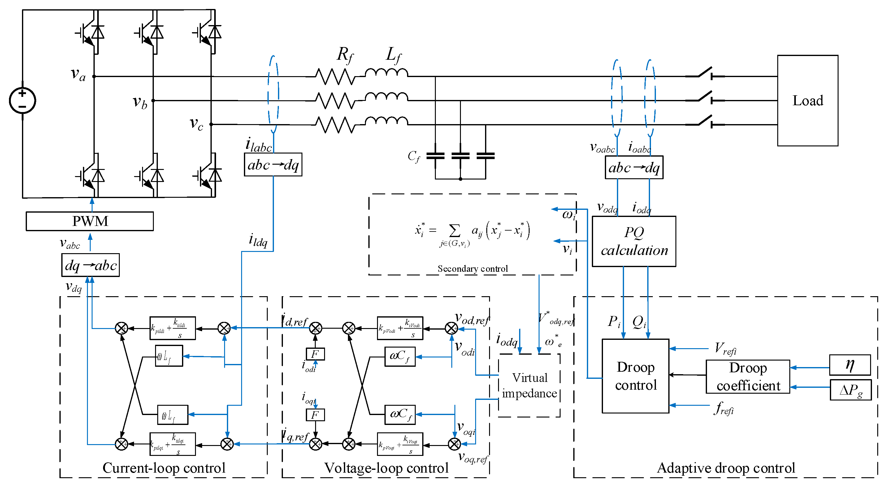
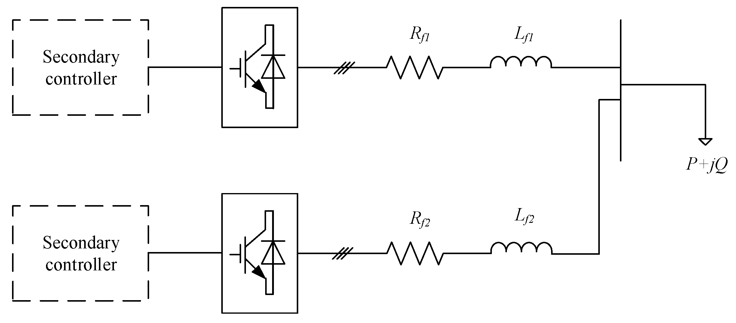
When microgrid system operates in islanded mode, the DG units are generally operated under droop control. With the disadvantages of inevitable frequency and voltage deviation caused by traditional droop control, there is always a secondary control to restore frequency and voltage in order to stabilize the system. The overall structure of control strategy for multi-DG microgrid is shown in Figure 1, including primary droop control for power sharing, inner voltage and current loops for generating PWM modulation signal and secondary control for the restoration of frequency and voltage amplitude. The control procedure is as follows: first, the adaptive fuzzy droop control is used as the primary control to manage the power sharing of each RES, which will cause a deviation in voltage magnitude and frequency. At the same time, the secondary control to restore voltage magnitude and frequency is completed by MAS controllers. The regulated voltage and frequency are sent to static virtual impedance loop, which is to eliminate the influence of line impedance. Then, the voltage will be transmitted to the double closed loops. The output (I_d,ref, I_q,ref) of the voltage loop is the input of the current loop. Finally, the output (V_d, V_q) of the current loop is used to make the PWM signal to control the operation of the DG.

2.1. Droop Control and Static Virtual Impedance

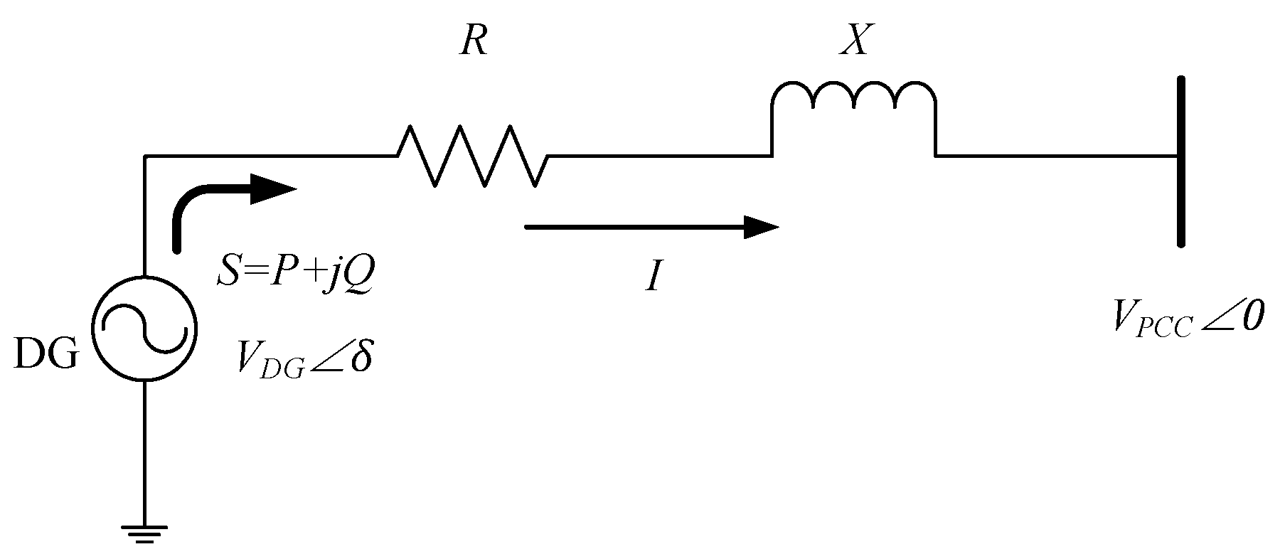
In order to balance the power sharing and increase system inertia, the conventional droop control method is widely used in microgrid. The basic droop control strategy can be illustrated in Figure 2, which is a simple diagram with a distributed generation (DG) connecting to the point of common coupling (PCC). In Figure 2, Z = R + jX is the line impedance, V_DG∠ δ is the output voltage of DG inverter, S = P + jQ is the power injection from DG to the main grid and V_PCC∠ 0 is the voltage of PCC.

Based on the current analysis theory, the power injection from DG to the main grid can be expressed as:

$$\begin{array}{cc}\hfill S=& P+jQ=V_{PCC}\angle 0\frac{V_{DG}\angle \delta -V_{PCC}\angle 0}{Z}\hfill \\ \hfill =& \frac{R\left(V_{DG}{V}_{PCC}\cos \delta -V_{DG}{}^2\right)+X{V}_{DG}{V}_{PCC}\sin \delta }{R^2+X^2}\hfill \\ & +j\frac{X\left(V_{DG}{V}_{PCC}\cos \delta -V_{DG}{}^2\right)-R{V}_{DG}{V}_{PCC}\sin \delta }{R^2+X^2}\hfill \end{array}$$

(1)

And then, the positive power and reactive power from DG can be expressed as:

$$P=\frac{R(V_{DG}{V}_{PCC}\cos \delta -V_{PCC}{}^2)+X{V}_{DG}{V}_{PCC}\sin \delta }{R^2+X^2}$$

(2)

$$Q=\frac{X(V_{DG}{V}_{PCC}\cos \delta -V_{PCC}{}^2)-R{V}_{DG}{V}_{PCC}\sin \delta }{R^2+X^2}$$

(3)

For those high-voltage and medium-voltage grids, the inductive characteristics are far stronger than the resistive characteristics, which is X>>R, so the positive power and reactive power can be rewritten as:

$$P=\frac{V_{DG}{V}_{PCC}\sin \delta }{X}$$

(4)

$$Q=\frac{V_{DG}{V}_{PCC}\cos \delta -V_{PCC}{}^2}{X}$$

(5)

Then, considering the phase angle difference between the output voltage of the DG unit and that of PCC is usually quite small, where sin δ ≈ δ, cos δ ≈ 1. So, the decoupling of positive power control and reactive power control can be realized, where positive power is proportional to the voltage phase angle difference (δ), which can be substituted by frequency and reactive power is proportional to the voltage amplitude difference (V_DC-V_PCC). And the active power-frequency (P-f) droop and reactive power-voltage (Q-v) droop can be expressed as follows:

$$f_i^{}=f_o-m_{pi}\cdot P_i$$

(6)

$$V_{DGi}^{}=V_{DGo}-m_{qi}\cdot Q_i$$

(7)

where i is the DG index, m_pi and m_qi are the droop coefficients represented active and reactive power, respectively, which are usually chosen based on the capacity of DG unit. V_DGi and f_i are voltage magnitude and frequency reference sent to the secondary control loop (where f_i is transformed in terms of ω_i). P_i and Q_i are the local output active and reactive power and the subscript “o” represents the rated operation points.

Despite the good performance in the inductive microgrid, when comes to the low-voltage microgrid where the line resistance cannot be ignored, the conventional droop control cannot decouple the positive power and reactive power, which will in turns cause an inaccurate power sharing and unstable operation. In order to eliminate the influence of line impedance, the virtual impedance is always needed. The advantages of virtual impedance are that it causes no power loss and increases the system performance by decoupling active power and reactive power if the parameters are designed properly.

With the static virtual output impedance loop, the voltage reference sent to PI voltage loop can be expressed as follows:

$$v_{odi,ref}=v_{odi,ref}^{*}-(R_{Vi}\cdot i_{odi}-X_{Vi}\cdot i_{oqi})$$

(8)

$$v_{oqi,ref}=v_{oqi,ref}^{*}-(R_{Vi}\cdot i_{oqi}+X_{Vi}\cdot i_{odi})$$

(9)

where v^*_odi,ref and v^*_oqi,ref are voltage references derived from U_i^* and f_i^*, which come from droop equations after an abc/dq transition, R_Vi and X_Vi represent the static virtual resistance and inductive impedance, respectively, i_odi and i_oqi are the output currents and the v_odi,ref and v_oqi,ref are voltage references sent to voltage loop controller.

2.2. Inner Control Strategy

The inner control loops mainly include voltage and current control loops. Typically, voltage and current control loops include feedback and feed-forward terms [22]. For the DG unit shown in Figure 1. The differential equation can be acquired based on the Kirchhoff’s current and voltage laws, after an abc/dq transition, the LCL filter can be expressed as:

$$\{\begin{array}{l}{v}_d=L_f\cdot {\dot{i}}_d+v_{od}+R_f\cdot i_d-{\mathsf{\omega }}_i\cdot L_f\cdot i_q\\ v_q=L_f\cdot {\dot{i}}_q+v_{oq}+R_f\cdot i_q+{\mathsf{\omega }}_i\cdot L_f\cdot i_d\end{array}$$

(10)

$$\{\begin{array}{l}{i}_d=C_f\cdot {\dot{v}}_{od}+i_{od}-{\mathsf{\omega }}_i\cdot C_f\cdot v_{oq}\\ i_q=C_f\cdot {\dot{v}}_{oq}+i_{oq}+{\mathsf{\omega }}_i\cdot C_f\cdot v_{od}\end{array}$$

(11)

where ω_i is the rotation speed of dq frame, L_f and R_f are respectively the inductance and resistance of the L filter and C_f is the capacitance of the C filter.

Based on the LCL filter, the voltage control methods can be expressed as follows:

$${\dot{\varphi }}_{odi}=v_{odi}^{*}-v_{odi},{\dot{\varphi }}_{oqi}=v_{oqi}^{*}-v_{oqi}$$

(12)

After the voltage control, there is:

$$\{\begin{array}{c}{i}_{ldi}^{*}=F{i}_{odi}-{\omega }_i{C}_f{v}_{oqi}+k_{pVodi}\left(v_{odi}^{*}-v_{odi}\right)+k_{iVodi}{\varphi }_{odi}\\ i_{lqi}^{*}=F{i}_{oqi}+{\omega }_i{C}_f{v}_{odi}+k_{pVoqi}\left(v_{oqi}^{*}-v_{oqi}\right)+k_{iVoqi}{\varphi }_{oqi}\end{array}$$

(13)

where F is the voltage control coefficient to improve stability.

The reference currents are sent to current control loop, which is:

$${\dot{\gamma }}_{di}=i_{ldi}^{*}-i_{ldi},{\dot{\gamma }}_{qi}=i_{lqi}^{*}-i_{lqi}$$

(14)

Then, the output of current control can be acquired, which are:

$$\{\begin{array}{c}{v}_{idi}^{*}=-{\omega }_i{L}_{fi}{i}_{lqi}+k_{pildi}\left(i_{ldi}^{*}-i_{ldi}\right)+k_{iildi}{\gamma }_{di}\\ v_{iqi}^{*}={\omega }_i{L}_{fi}{i}_{ldi}+k_{pilqi}\left(i_{lqi}^{*}-i_{lqi}\right)+k_{iilqi}{\gamma }_{qi}\end{array}$$

(15)

Then after a dq/abc transition, the PWM modulation signal can be obtained. These controllers can effectively reduce the resonance effects caused by droop control and in turns to improve the system stability.

2.3. Secondary Control Strategy

When the power generation and power demand have a mismatch, the output voltage reference of DG unit with conventional droop control will have a deviation from the rated value, both in frequency and amplitude. The secondary control is designed to guarantee the restoration of frequency and voltage after droop control, in turns keep the system stable under uncertain circumstances such as load change.

First some notations and preliminaries that are used in this paper are defined for the following analysis.

A directed graph G = (V, E, A) is defined to explain the system topology, where $V(G)=\left\{v_1,v_2\cdots ,v_n\right\}$ donates the node set which contains load and DG units, $E(G)=\left\{(v_i,v_j):i,j\in (1,\dots ,n)\right\}$ donates the edge set. The fact that node i can communicate with node j means that $(v_j,v_i)\in E(G)$, which also means that node i is a neighbor of node j. For a directed graph G, its adjacency $A\in R_{}^{\left|V\right|\times \left|V\right|}$ is defined by a_ii = 0, a_ij = 1 when $(v_j,v_i)\in E(G)$ and a_ij = 0 otherwise.

The impedance matrix is defined as $Y\in j{R}_{}^{n\times n}$ and the voltage magnitude of node i: $E_i>0$, based on the circuit theory, the line weighted matrix is $C=diag\left({\left\{c_{ij}\right\}}_{\left\{i,j\right\}\in \epsilon }\right)$, where $c_{ij}=E_i{E}_j\left|Y_{ij}\right|$. And matrix B is defined to represent the relationship of node and edge, $B_{}^{T}x\in R_{}^{\left|E\right|}$ represents $x_i-x_j$ when $\left\{i,j\right\}\in \epsilon$.

Based on the distributed multi-agent system, the secondary control is designed to restore the deviation of voltage magnitude and frequency. The basic idea is to realize the synchronization of voltage and frequency, which can be divided into two parts: first the initial value of all DGs should be consistent and then during the system operation the reference value can be sent to every DG.

As the microgrid is operated in islanded mode, there is no leader information from the main grid, so the reference value x_i^* is the average value of all DG, which is $x_{avg}^{*}=\frac{1}{\left|N\right|}{\displaystyle \sum _{i\in N}{x}_i^{*}}$, where x_i^* means frequency or voltage. The basic idea of multi-agent system is:

$${\dot{x}}_i^{*}={\displaystyle \sum _{j\in (G,v_i)}{a}_{ij}\left(x_j^{*}-x_i^{*}\right)}$$

(16)

Take frequency control as an example, considering communication delay, the consistency controller is:

$$e_i\left(t\right)=-{\displaystyle \sum _{j\in N(G,v_i)}^{}{a}_{ij}\left[\frac{P_i^{}\left(t-{\tau }_1\right)}{d_i}-\frac{P_j^{}\left(t-{\tau }_2\right)}{d_j}\right]}$$

(17)

where τ₁ represents calculation delay, τ₂ represents the sum of communication delay and calculation delay and d represents the weighted degree as $d_i={\displaystyle \sum _{i=1}^N{a}_{ij}}$.

The control variable u_i(t) can be obtained when the error $e_i\left(t\right)$ is regulated by a PI controller. Then system with secondary control can be expressed as:

$$D\dot{\delta }\left(t\right)=P^{*}-BC\sin \left(B_{}^T\delta \left(t\right)\right)-Du\left(t\right)$$

(18)

where $D=diag\left(0_{\left|{\nu }_L\right|},{\left\{d_i\right\}}_{i\in {\nu }_{DG}}\right)$.

Similarly, the consistency of voltage magnitude can be obtained.

Remark: 

After the above control strategy, the microgrid can realize a stable operation with a balanced power sharing and frequency/voltage synchronized with the rated value regardless of line impedance and load variation. However, the characteristics of RES, such as power fluctuation of generation units, will cause an impact on system stability, which will be discussed in the following section.

3. Adaptive Fuzzy Droop Control

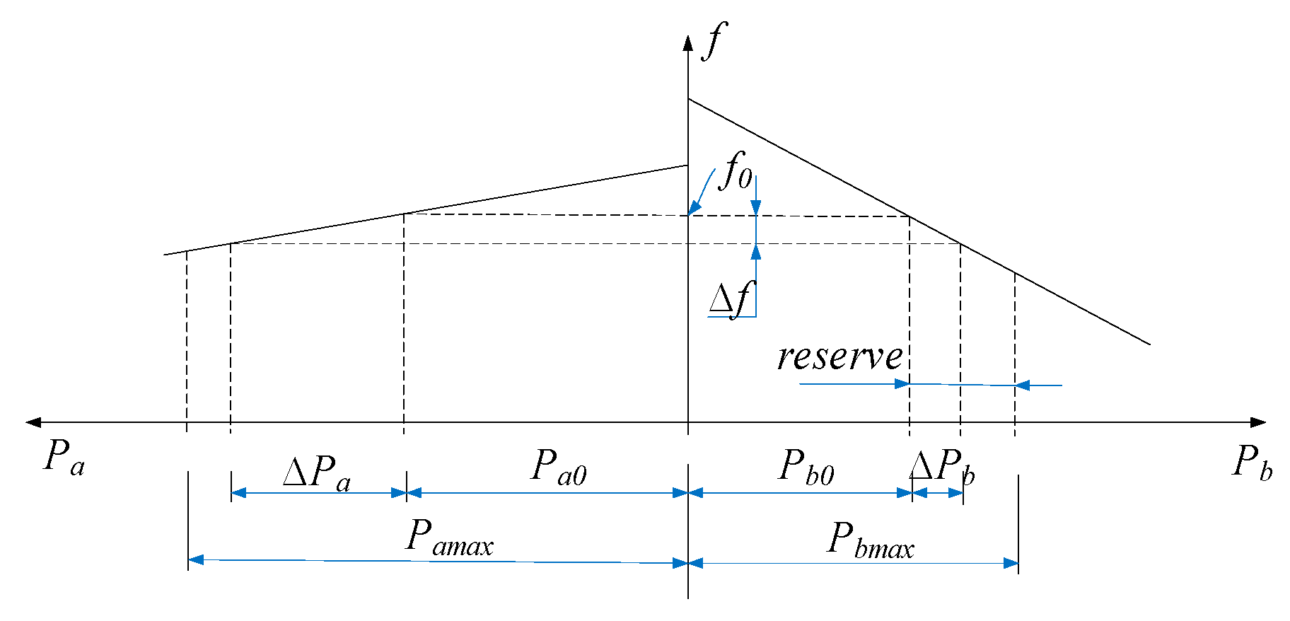
The conventional droop can provide primary frequency regulation, which imitates the operation of a synchronous machine. Take P-f droop control for example, the relationship between frequency and positive power sharing is:

$$\frac{\Delta \mathsf{\omega }}{{\mathsf{\omega }}_0}=-{\mathrm{m}}_P\frac{\Delta P_m}{P_0}$$

(19)

where m_P is the droop coefficient, ∆ω = ω − ω_ref represents the change of frequency and ∆P_m represents the change of power output according to the frequency change. This relationship is illustrated in Figure 3 with two RESs. When the load increases, the system can rebuild the generation/demand balance with droop characteristics, where frequency drops and output power increases. The power sharing between RESs applies the following rules: one that with smaller m_P is responsible for a larger power share (i.e., ∆P_b < ∆P_a in Figure 3).

The droop control is widely used in microgrids for its reliability. However, with the power fluctuation of RES, the reserve energy is always uncertain, which makes droop control hard to stabilize the system. So, the PQ operation mode, where the output power can be acquired from a maximum power point tracking algorithm, is a popular option for RES for (1) the maximum power output can be realized and (2) energy reserves for frequency regulation are not necessary. But with the islanded operation mode, there will be no frequency support from the main grid, so there must be some equipment to offer frequency regulation, commonly the energy storage systems (ESS). However, with the increasing of RES in the microgrid, the responsibility of frequency regulation may go beyond the ability of ESS and it may not be able to guarantee the power balance under extreme circumstances such as enormous generation fluctuation. What is more, the usage of ESS will increase the operation cost of the microgrid. So, an adaptive droop coefficient for RES units to participate in frequency regulation and optimized power sharing is needed.

For a microgrid, the design of droop coefficient, m_P, is usually based on the equitable power sharing, which is:

$$m_{P1}{P}_1=m_{P2}{P}_2=\cdots =const$$

(20)

where P_i is the output power of the ith RES.

In traditional droop control, the droop coefficient is designed only based on the inverter capacity, which is not accurate when generation units have a power fluctuation. So, it should be adjusted based on the real-time power capacity of RES itself, in case of power overloading/curtailment.

If the RES has a sudden power reduction, the droop coefficient should be adjusted to decrease its output power, which means other RESs which have a larger power reserve will increase output power to rebuild the generation/demand balance. In this situation, the priority of designing droop coefficient is to ensure the system stability, where the RES should operate within its maximum power capacity.

What is more, the generation/demand relationship should be considered when designing the droop coefficient. When the power demand is quite low compared with the rated power generation (particularly referring to RES capacity) in real-time, the RES should be assigned a smaller droop coefficient to realize a larger power output with less energy waste, where the other equipment as ESS or fossil-fuel power generation units should decrease their output to reduce operation cost. This is the time when economic power sharing should be considered.

On the other hand, when the demand increases, the energy reserve will decrease and the necessity of frequency regulation calls for a larger droop coefficient, where the system stability is the prior objective. Therefore, the main consideration for coefficient selection is the power deviation, which represents the power fluctuation and the power balance, which represents the relationship between real-time power demand and rated power generation.

Fuzzy logic controller is suitable for the system with uncertainties, for it does not need a mathematical model and can realize a multi-objective optimization [23,24]. The fuzzy logic method can get the experience and knowledge of an expert to predict the system behavior, which is helpful in selecting the adaptive droop coefficient. It can be designed by requiring the power deviation and power balance, updating the droop coefficient and then realizing the optimized power sharing among RES considering stability and economics.

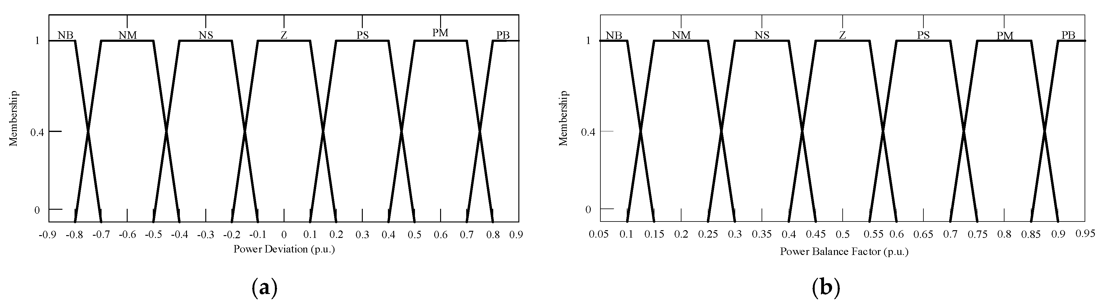
The triangle membership function is widely used in fuzzy logic system for its simplicity. However, the result of triangle membership is most likely a point value, where a different input value corresponds to a different output value, which is not accurate for the situation where the parameters are flat distributed. Compared with the triangle membership function, the trapezoidal-shaped membership function provides that the different input interval corresponds to a different result value, which is more suitable for droop coefficient regulation because the droop coefficient cannot be changed too frequently for the fear that the system stability is affected.

There are three different parameters in triangle membership function considering a single membership value, which are the minimum input value, the peak input value and the maximum input value. As for trapezoidal-shaped membership function, there are four different parameters because the peak input interval needs two input points. So, the trapezoidal-shaped membership is more flexible and more accurate. The design of input parameters is first obtained on the basis of expert experience then adjusted according to numeral simulations. As shown in Figure 4, the input variables of fuzzy logic control are the power deviation ΔP $=\frac{P_{N,t+1}-P_{N,t}}{P_{N,t}}$, where t represents the sampling time and the power balance factor η = $\frac{{\displaystyle \sum _{i=1}^n{P}_{GNi}}}{P_L}$. The range of η is limited from 5% to 95%.

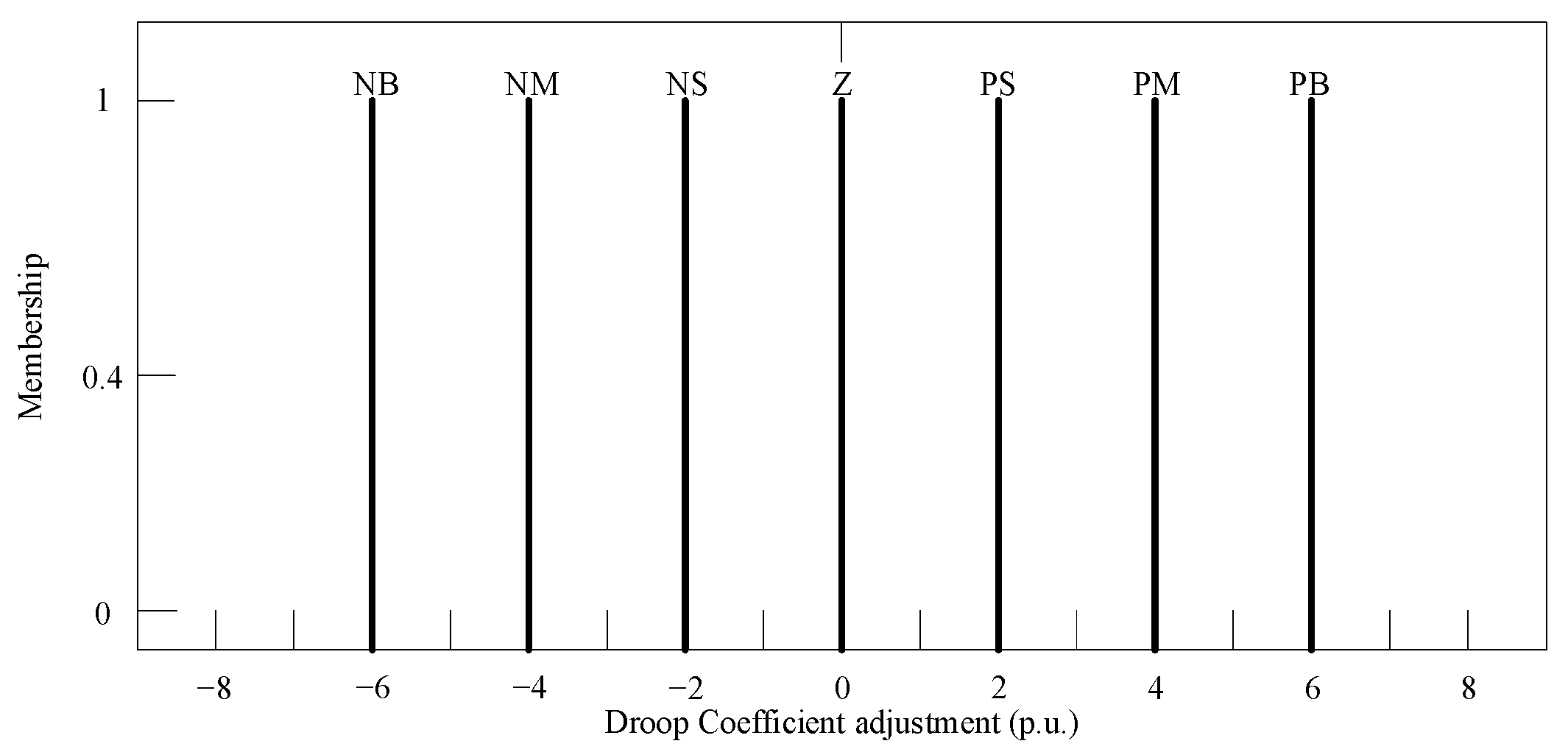
The influence of power deviation and power balance factor on droop coefficient is determined by the membership grade, which is expressed by linguistic variables: negative big (NB), negative medium (NM), negative small (NS), zero (Z), positive medium (PM), positive small (PS) and positive big (PB). The fuzzy membership functions for power deviation ΔP and power balance factor η, as well as the droop coefficient m_P are respectively shown in Figure 5 and Figure 6.

Take input power deviation ∆P for example, the trapezoidal-shaped membership function for ∆P corresponding to NM is defined as:

$$f(\Delta P;\Delta P_{\min },\Delta P_{NM\min },\Delta P_{NM\max },\Delta P_{\max })=\{\begin{array}{ll}0,\hfill & \Delta P\le \Delta P_{\min }\hfill \\ \frac{\Delta P-\Delta P_{\min }}{\Delta P_{NM\min }-\Delta P_{\min }},\hfill & \Delta P_{\min }<\Delta P\le \Delta P_{NM\min }\hfill \\ 1,\hfill & \Delta P_{NM\min }<\Delta P\le \Delta P_{NM\max }\hfill \\ \frac{\Delta P_{\max }-\Delta P}{\Delta P_{\max }-\Delta P_{NM\max }},\hfill & \Delta P_{NM\max }<\Delta P\le \Delta P_{\max }\hfill \\ 0,\hfill & \Delta P>\Delta P_{\max }\hfill \end{array}$$

(21)

where the parameters ΔP_min, ΔP_NMmin, ΔP_NMmax and ΔP_max are chosen based on the influence of power deviation to the system operation. According to Figure 5, ΔP_min = −0.8, ΔP_NMmin = −0.7, ΔP_NMmax = −0.5 and ΔP_max = −0.4. The membership function of power balance factor η can also be seen in Figure 5. And the single-value function can be understood clearly in Figure 6.

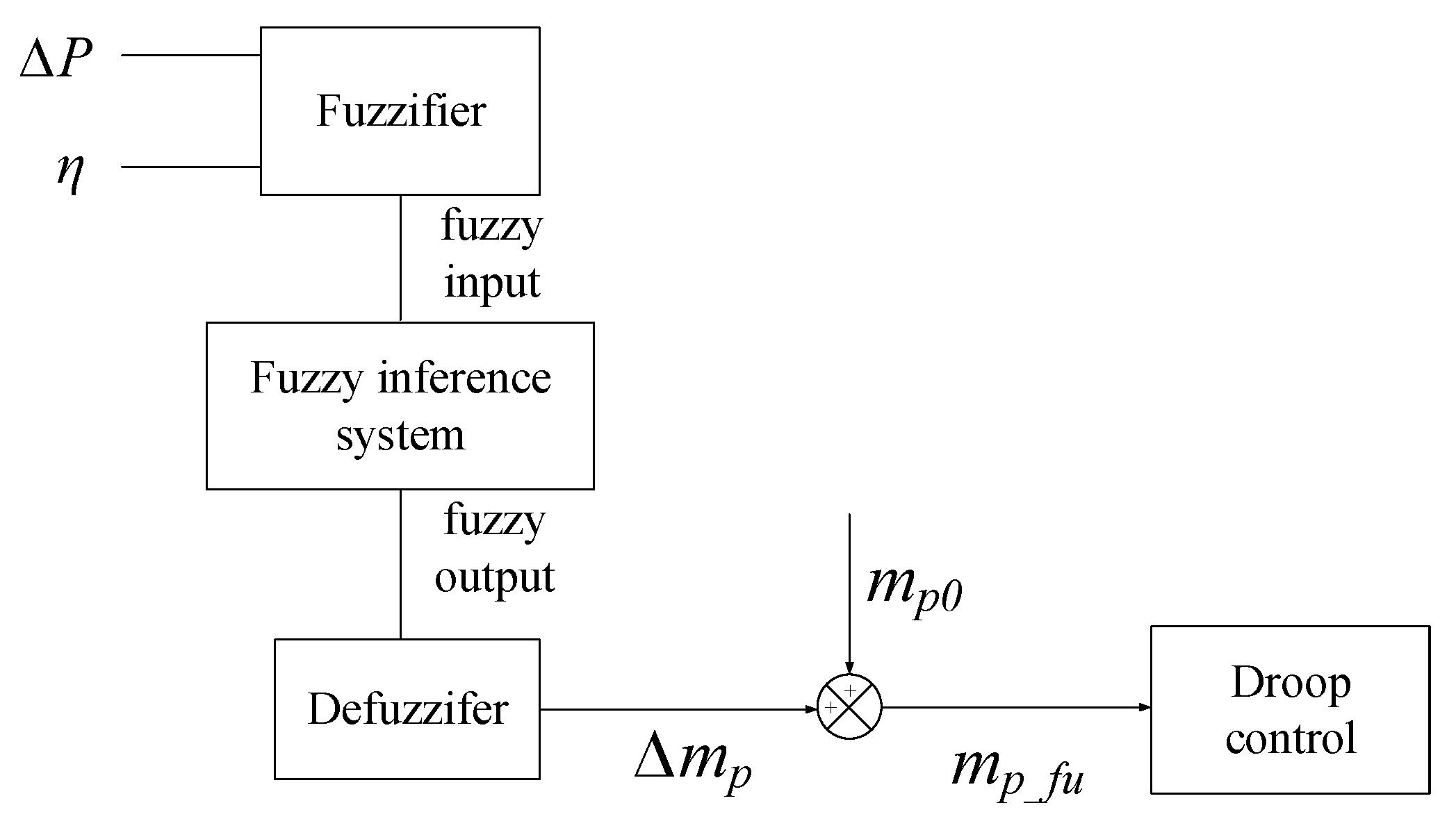
After the fuzzifier which turns the input parameters into membership grades, there should be detailed fuzzy rules to determine the influence of input variables on output variable. The adjustment of droop coefficient m_p is based on the fuzzy logic controller. Depending on the power balance factor η and the power deviation ∆P, the m_p can be increased and decreased. The basic fuzzy inference rule is: when the power balance factor is relatively low, the droop coefficient should be decreased so that the RES can provide more power output because there can be less power reserve and the output power can be as much as the maximum value. Otherwise, when the power balance factor becomes high, the system stability will be the prior objective where the droop coefficient should be adjusted mainly according to the power deviation. The negative power deviation will cause an increase in droop coefficient because of the decrease in power reserve. When the power balance factor is in the medium value (i.e., 0.4 < η < 0.6), the adjustment of m_p will be determined by both two factors. The fuzzy logic rules are listed in

Table 1. Rules for Fuzzy Controllers.

Droop Coefficient		Power Balance Factor
		NB	NM	NS	Z	PS	PM	PB
Power Deviation	NB	NB	NM	PM	PB	PB	PB	PB
	NM	NB	NM	PS	PM	PB	PM	PM
	NS	NB	NM	Z	PS	PM	PS	PS
	Z	NB	NM	NS	Z	PS	Z	Z
	PS	NB	NM	NM	NS	Z	NS	NS
	PM	NB	NM	NB	NM	NS	NM	NM
	PB	NB	NM	NB	NB	NM	NB	NB

. Based on the fuzzy rule, by using the mamdani fuzzy model with minimum and maximum relations, the output variable can be calculated.

By using the fuzzy inference and defuzzification, a nonfuzzy output, ∆m_p, is acquired, which can be added to the initial droop coefficient, m_p0, which is:

$$m_{p\_fu}=m_{p0}+\Delta m_p$$

(22)

Applying (22) to (6), which is:

$$f_i^{*}=f_o-m_{pi\_fu}\cdot P_i$$

(23)

And the output positive power of RES can be regulated based on (23).

There are other adaptive control methods such as PID controllers, however, it is hard for PID controller to realize a multi-objective control with little calculation for the coupling of multiple input variables is hard to evaluate. The proposed AFDC is based on the expert experience and numeral simulations, which means it is easy to evaluate the relationship of each input variables. And the fuzzy rules are designed to illustrate the relationship of the input and output, which is quicker than PID controller and more accurate.

4. Stability Analysis

The droop control impacts the stability of the microgrid system. As for a fixed control coefficient, the stability analysis seems unnecessary because the selection of the parameter considers the stability constrain. However, an adaptive droop coefficient may affect the stability, hence a stability region for regulation should be determined. Moreover, the dynamic characteristics of the primary and secondary control should be analyzed to better illustrate the stability feature of the proposed strategy. The eigenvalues analysis is used to evaluate the impact of droop coefficient on stability and the Lyapunov function is used to evaluate the impact of proposed control strategy with secondary control.

4.1. Eigenvalues Analysis

Based on the droop control methods containing P-f and Q-v droop strategies, combining the inner double-loop controller, the model of inverter can be derived. Then the small-signal model can be obtained by linearization methods around a nominal condition, according to which the root locus can be calculated.

The small-signal model of the microgrid with droop control can be obtained in Reference [25], which can be expressed in state-space form as:

$$\Delta \dot{X}=A\Delta X$$

(24)

where X is the state vector and A is the state matrix that contains the necessary information of the small-signal stability of the system.

The eigenvalue analysis is performed to determine the small-signal stability of the microgrid system and to restrict the stability region of the droop coefficient. The fact that the system has positive eigenvalues means the instability and vice versa. The root locus of the system with the droop coefficient change is shown in Figure 7. As shown in Figure 7, the control strategy can be stable if and only if there are no right-hand planes (RHPs) of the minor loop gain. So, the system can be stable when droop coefficient m_p changing from 10⁻⁶ to 1.5 × 10⁻⁴ and m_q changing from 10⁻⁶ to 3.6×10⁻⁴. When the droop coefficient exceeds the stability region, the eigenvalues will move from the left-hand plane to the right-hand plane, which results in the instability of the system. It can be clear seen that the droop coefficient has a wide operation range that guarantees the system stability.

4.2. Lyapunov Stability

Take the frequency secondary controller as an example, the Lyapunov stability is analyzed to prove the system stability. The system (17) can be rewritten as:

$$e\left(t\right)=\dot{\tilde{P}}\left(t\right)=-I\tilde{P}\left(t-{\tau }_1^{}\right)+A\tilde{P}\left(t-{\tau }_2^{}\right)$$

(25)

where $\tilde{P}\left(t-{\tau }_1^{}\right)={\left[\frac{P_1\left(t-{\tau }_1^{}\right)}{d_1},\dots ,\frac{P_{\left|V_I\right|}\left(t-{\tau }_1^{}\right)}{d_{\left|V_I\right|}}\right]}_{}^T$, $\tilde{P}\left(t-{\tau }_2^{}\right)={\left[\frac{P_1\left(t-{\tau }_2^{}\right)}{d_1},\dots ,\frac{P_{\left|V_I\right|}\left(t-{\tau }_2^{}\right)}{d_{\left|V_I\right|}}\right]}_{}^T$.

Theorem: 

As for a time delay ${\tau }_i\ge 0\left(i=1,2\right)$ satisfying ${\tau }_2>{\tau }_1$, if there exists positive definite matrixes $P=P^T$ and $Q_i=Q_i^T$ (i = 1, 2) and semi-positive definite matrixes $W_i=W_i^T$, $W_i=W_i^T$, $Y_{ii}=Y_{ii}^T$ and $Z_{ii}=Z_{ii}^T$ (i = 1, 2, 3) and arbitrary matrixes $N_i$, $S_i$, $T_i$ $\left(i=1,2,3\right)$ and $X_{ij},Y_{ij},Z_{ij}\left(1\le i<j\le 3\right)$, the system can be stable when the following LMI is satisfied.

$$\mathsf{\Phi }=\left[\begin{array}{ccc}{\varphi }_{11}& {\varphi }_{12}& {\varphi }_{13}\\ {\varphi }_{12}^T& {\varphi }_{22}& {\varphi }_{23}\\ {\varphi }_{13}^T& {\varphi }_{23}^T& {\varphi }_{33}\end{array}\right]<0$$

(26)

$${\mathsf{\Psi }}_1=\left[\begin{array}{cccc}{X}_{11}& X_{12}& X_{13}& N_1\\ X_{12}^T& X_{22}& X_{23}& N_2\\ X_{12}^T& X_{23}^T& X_{33}& N_3\\ N_1^T& N_2^T& N_3^T& W_1\end{array}\right]\ge 0$$

(27)

$${\mathsf{\Psi }}_2=\left[\begin{array}{cccc}{Y}_{11}& Y_{12}& Y_{13}& S_1\\ Y_{12}^T& Y_{22}& Y_{23}& S_2\\ Y_{12}^T& Y_{23}^T& Y_{33}& S_3\\ S_1^T& S_2^T& S_3^T& W_2\end{array}\right]\ge 0$$

(28)

$${\mathsf{\Psi }}_3=\left[\begin{array}{cccc}{Z}_{11}& Z_{12}& Z_{13}& k{T}_1\\ Z_{12}^T& Z_{22}& Z_{23}& k{T}_2\\ Z_{12}^T& Z_{23}^T& Z_{33}& k{T}_3\\ k{T}_1^T& k{T}_2^T& k{T}_3^T& W_3\end{array}\right]\ge 0$$

(29)

where:

• ${\varphi }_{11}=Q_1+Q_2+N_1+N_1^T+S_1+S_1^T+H+{\tau }_1{X}_{11}+{\tau }_2{Y}_{22}+\left({\tau }_2-{\tau }_1\right)Z_{11}$
• ${\varphi }_{12}=P{A}_1-N_1+N_2^T+S_2^T+T_1+H+{\tau }_1{X}_{12}+{\tau }_2{Y}_{12}+\left({\tau }_2-{\tau }_1\right)Z_{12}$
• ${\varphi }_{13}=P{A}_2+N_3^T-S_1+S_3^T-T_1+H+{\tau }_1{X}_{13}+{\tau }_2{Y}_{13}+\left({\tau }_2-{\tau }_1\right)Z_{13}$
• ${\varphi }_{22}=-Q_1-N_2-N_2^T+T_2+T_2^T+H+{\tau }_1{X}_{22}+{\tau }_2{Y}_{22}+\left({\tau }_2-{\tau }_1\right)Z_{22}$
• ${\varphi }_{23}=-N_3^T-S_2-T_2+T_3^T+H+{\tau }_1{X}_{23}+{\tau }_2{Y}_{23}+\left({\tau }_2-{\tau }_1\right)Z_{23}$
• ${\varphi }_{23}=-Q_2-S_3-S_3^T-T_3-T_3^T+H+{\tau }_1{X}_{33}+{\tau }_2{Y}_{33}+\left({\tau }_2-{\tau }_1\right)Z_{33}$
• $H={\tau }_1{W}_1+{\tau }_2{W}_2+\left({\tau }_2-{\tau }_1\right)W_3$

Proof: 

The following Lyapunov-Krasovskii function is chosen for stability analysis:

$$\begin{array}{cc}{V}_1& ={\tilde{P}}^T\left(t\right)P\tilde{P}\left(t\right)+{\displaystyle {\int }_{t-{\tau }_1}^t{\tilde{P}}^T\left(s\right)Q_1\tilde{P}\left(s\right)ds}+{\displaystyle {\int }_{t-{\tau }_2}^t{\tilde{P}}^T\left(s\right)Q_2\tilde{P}\left(s\right)ds}\hfill \\ & +{\displaystyle {\int }_{-{\tau }_1}^0{\displaystyle {\int }_{t+\theta }^t{\dot{\tilde{P}}}^T\left(s\right)W_1\dot{\tilde{P}}\left(s\right)ds}}d\theta +{\displaystyle {\int }_{-{\tau }_2}^0{\displaystyle {\int }_{t+\theta }^t{\dot{\tilde{P}}}^T\left(s\right)W_2\dot{\tilde{P}}\left(s\right)ds}}d\theta \hfill \\ & +{\displaystyle {\int }_{-{\tau }_2}^{-{\tau }_1}{\displaystyle {\int }_{t+\theta }^t{\dot{\tilde{P}}}^T\left(s\right)W_3\dot{\tilde{P}}\left(s\right)ds}}d\theta \hfill \end{array}$$

(30)

where $P=P^T>0$, $Q_i=Q_i^T>0\left(i=1,2\right)$, $W_i=W_i^T\ge 0 \left(i=1,2,3\right)$.

And then calculates the derivative of (30):

$$\begin{array}{ll}{\dot{V}}_1\hfill & =2{\tilde{P}}^T\left(t\right)P\left[-I\tilde{P}\left(t-{\tau }_1\right)+A\tilde{P}\left(t-{\tau }_2\right)\right]\hfill \\ & +{\tilde{P}}^T\left(t\right)Q_1\tilde{P}\left(t\right)-{\tilde{P}}^T\left(t-{\tau }_1\right)Q_1\tilde{P}\left(t-{\tau }_1\right)\hfill \\ & +{\tilde{P}}^T\left(t\right)Q_2\tilde{P}\left(t\right)-{\tilde{P}}^T\left(t-{\tau }_2\right)Q_2\tilde{P}\left(t-{\tau }_2\right)\hfill \\ & +{\tau }_1{\dot{\tilde{P}}}^T\left(t\right)W_1\dot{\tilde{P}}\left(t\right)-{\displaystyle {\int }_{t-{\tau }_1}^t{\dot{\tilde{P}}}^T\left(s\right)W_1\dot{\tilde{P}}\left(s\right)ds}\hfill \\ & +{\tau }_2{\dot{\tilde{P}}}^T\left(t\right)W_2\dot{\tilde{P}}\left(t\right)-{\displaystyle {\int }_{t-{\tau }_2}^t{\dot{\tilde{P}}}^T\left(s\right)W_2\dot{\tilde{P}}\left(s\right)ds}\hfill \\ & +\left({\tau }_2-{\tau }_1\right){\dot{\tilde{P}}}^T\left(t\right)W_3\dot{\tilde{P}}\left(t\right)-{\displaystyle {\int }_{t-{\tau }_2}^{t-{\tau }_1}{\dot{\tilde{P}}}^T\left(s\right)W_3\dot{\tilde{P}}\left(s\right)ds}\hfill \end{array}$$

(31)

Based on Leibniz-Newton function, for arbitrary matrixes $N_i$, $S_i$, $T_i=T_i^T\ge 0 \left(i=1,2,3\right)$, there are:

$$2\left[{\tilde{P}}_{}^T\left(t\right)N_1+{\tilde{P}}_{}^T\left(t-{\tau }_1\right)N_2+{\tilde{P}}_{}^T\left(t-{\tau }_2\right)N_3\right]\times \left[\tilde{P}\left(t\right)-\tilde{P}\left(t-{\tau }_1\right)-{\displaystyle {\int }_{t-{\tau }_1}^t\dot{\tilde{P}}\left(s\right)ds}\right]=0$$

(32)

$$2\left[{\tilde{P}}_{}^T\left(t\right)S_1+{\tilde{P}}_{}^T\left(t-{\tau }_1\right)S_2+{\tilde{P}}_{}^T\left(t-{\tau }_2\right)S_3\right]\times \left[\tilde{P}\left(t\right)-\tilde{P}\left(t-{\tau }_2\right)-{\displaystyle {\int }_{t-{\tau }_2}^t\dot{\tilde{P}}\left(s\right)ds}\right]=0$$

(33)

$$2\left[{\tilde{P}}_{}^T\left(t\right)T_1+{\tilde{P}}_{}^T\left(t-{\tau }_1\right)T_2+{\tilde{P}}_{}^T\left(t-{\tau }_2\right)T_3\right]\times \left[\tilde{P}\left(t-{\tau }_1\right)-\tilde{P}\left(t-{\tau }_2\right)-{\displaystyle {\int }_{t-{\tau }_2}^{t-{\tau }_1}\dot{\tilde{P}}\left(s\right)ds}\right]=0$$

(34)

As for any matrix with the same dimension, $X_{ii}=X_{ii}^T\ge 0$, $Y_{ii}=Y_{ii}^T\ge 0$, $Z_{ii}=Z_{ii}^T\ge 0$ $\left(i=1,2,3\right)$, $X_{ij},Y_{ij},Z_{ij}\left(1\le i<j\le 3\right)$, there is:

$${\left[\begin{array}{c}\tilde{P}\left(t\right)\\ \tilde{P}\left(t-{\tau }_1\right)\\ \tilde{P}\left(t-{\tau }_2\right)\end{array}\right]}^T\left[\begin{array}{ccc}{\mathsf{\Lambda }}_{11}& {\mathsf{\Lambda }}_{12}& {\mathsf{\Lambda }}_3\\ {\mathsf{\Lambda }}_{12}^T& {\mathsf{\Lambda }}_{22}& {\mathsf{\Lambda }}_{23}\\ {\mathsf{\Lambda }}_{13}^T& {\mathsf{\Lambda }}_{23}^T& {\mathsf{\Lambda }}_{33}\end{array}\right]\left[\begin{array}{c}\tilde{P}\left(t\right)\\ \tilde{P}\left(t-{\tau }_1\right)\\ \tilde{P}\left(t-{\tau }_2\right)\end{array}\right]=0$$

(35)

where ${\mathsf{\Lambda }}_{ij}={\tau }_1\left(X_{ij}-X_{ij}\right)+{\tau }_2\left(Y_{ij}-Y_{ij}\right)+\left|{\tau }_1-{\tau }_2\right|\left(Z_{ij}-Z_{ij}\right), 1\le i\le j\le 3$.

Add (31) to the left side of (32)–(35), then (31) can be rewritten as:

$$\begin{array}{cc}{\dot{V}}_1& ={\eta }_1^T\left(t\right)\mathsf{\Phi }\eta \left(t\right)-{\displaystyle {\int }_{t-{\tau }_1}^t{\eta }_2^T}\left(t,s\right){\mathsf{\Psi }}_1{\eta }_2\left(t,s\right)ds\hfill \\ & -{\displaystyle {\int }_{t-{\tau }_2}^t{\eta }_2^T}\left(t,s\right){\mathsf{\Psi }}_2{\eta }_2\left(t,s\right)ds-{\displaystyle {\int }_{t-{\tau }_2}^{t-{\tau }_1}{\eta }_2^T\left(t,s\right)}{\mathsf{\Psi }}_3{\eta }_2\left(t,s\right)ds\hfill \end{array}$$

(36)

where ${\eta }_1\left(t\right)={\left[\begin{array}{ccc}{\tilde{P}}^T\left(t\right)& {\tilde{P}}^T\left(t-{\tau }_1\right)& {\tilde{P}}^T\left(t-{\tau }_2\right)\end{array}\right]}^T$, ${\eta }_2\left(t,s\right)={\left[\begin{array}{cc}{\eta }_1^T\left(t\right)& {\dot{\tilde{P}}}^T\left(s\right)\end{array}\right]}^T$.

So, the system is asymptotic stable for arbitrary ${\eta }_1\left(t\right)\ne 0$ when $\mathsf{\Phi }<0$ and ${\mathsf{\Psi }}_i\ge 0 \left(i=1,2,3\right)$.

5. Simulation Results

As for the system configuration and parameters shown in Figure 8, the system model is built in MATLAB/Simulink. The secondary control provides frequency and voltage restoration and the primary droop control concludes the fuzzy-based droop coefficient adjustment. In the first simulation case, there are two RES applied droop control to realize a balanced power sharing and responsible for frequency regulation. In order to reasonably simplify the simulation, the RES is represented by alterable DC power, where detailed data is shown in

Table 2. Parameters of Microgrid System.

Item	Value
Microgrid Parameters
RES1	20 kW
RES2	20 kW
ZLine1	0.2 + j0.0006 Ω
ZLine2	0.175 + j0.00095 Ω
L,C Rated Frequency Rated voltage	1.8 mH, 50 μF 60 Hz 208 V
Primary Control Parameters
mp1	2.18e−5
mp2	2.18e−5
kpi1, kpr1	1, 100
kpi2, kpr2	50, 500
Rvi, Lvi	0.1Ω, 1.8e−3 mH
Secondary Control Parameters
kPf, kiF	0.5e−3, 0.1
kPE, kiE	0.1e−3, 0.11

. In the second simulation case, a RES unit, which is wind power or photovoltaic power, is paralleled with a traditional power unit to supply a variable load. The generation information of wind power is the realistic data from HaoGuanying wind farm and that of photovoltaic power is from a photovoltaic power station in Liaoning Province in China. In simulation case 2, except for the rated power capacity, the parameters of controller and topology are the same with Table 2.

5.1. Case 1: Two Paralleled RES

In this simulation case, the validity of the fundamental control strategy will be illustrated, where the proposed adaptive control method will be operated under the circumstances where the load and generation changes and will be compared with the traditional droop method.

5.1.1. Variation in Load

In this situation, two DGs are considered having adequate power reserve whose power fluctuation can be ignored. The capacity of DG 1 is the same with that of DG 2.

As shown in Figure 9a,b, in the first stage (0–0.6 s), the power demand is 25 kW and each DG has an equal power sharing, 11 kW considering the line loss. With droop control methods, the frequency has a slight drop from 60.4 Hz to 60.2 Hz to cover the power demand. The output voltage is stable at 208 V and the current is stable at around 50 A.

At 0.6 s, the load increases by 15 kW. With the sudden load increase, output power increases to realize the power balance and eliminate the power mismatch. Because of the same capacity, the output power of each DG increase by 5 kW, where a new power balance can be reached. However, in order to realize a larger power output, the frequency has a drop from 60.2 Hz to 60.1 Hz, which in the end can reach to the consensus.

At 0.6 s, the voltage has an instant slight decrease following the sudden load change, which can return its rated value by the secondary control. The output current increased following the increase in power demand.

By the adaptive droop control, the output power of RES unit can be followed with the change of power load. A new power balance can be reached within 0.3 s, which is acceptable considering the operation of microgrid. The output voltage can be stable with the amplitude within the error and output current can be increased to boost the output power. The frequency of the microgrid has changed to balance the power mismatch under the droop control and eventually converged to the stable value.

5.1.2. Variation in Generation

In this situation, the power demand is considered constant and the capacity of RES changes so that the power reserve changes, where the droop coefficient should be adjusted in case of power overloading/curtailment. The initial capacity of RES1 and RES2 is 2:1, which will become 1:1 at 0.6 s and the power demand remains 25 kW during the simulation period.

As shown in Figure 10a–c, in the first stage (0–0.6), the output power of DG1 is 14 kW and that of DG2 is 7 kW, which is proportional with its own capacity. With droop control, DG1, having a larger power reserve, has a larger frequency drop from 60.8 Hz to 60.2 Hz, then has a slightly frequency recover to 60.3 Hz and DG2 has a smaller frequency drop from 60.4 Hz to 60.3 Hz, which resulting from the difference in droop coefficient.

At 0.6 s, the capacity of DG1 decreases by 50%, which means both two DGs have a same capacity. The power reserve of DG1 has decreased, so the droop coefficient should be adjusted so there will not be a power overloading to DG1. With the droop coefficient of DG1 increased by 50%, the output power of DG1 and DG2 are the same, they have an equal power sharing at 10.5 kW. When the droop coefficient of DG1 changes at 0.6 s, the frequency of DG1 has an instant change from 60.3 Hz to 60.1 Hz and relatively the output power changes slowly. With the constant power load, the output voltage and current remain stable.

With the adaptive droop control, the output power of RES unit can be proportional with its own capacity by adjusting droop coefficient, which can be seen in Figure 9d. The frequency of the microgrid can be converged to the stable value and the new power balance can be reached within 0.3 s, which is acceptable.

5.1.3. Variation in Load and Generation

There will be no constant power load or power generation, especially for RES unit with frequent power fluctuation. The above two simulations analysis the situation with constant power load and constant power generation, which will be combined in this simulation. The droop coefficient will decrease when power load increases and it will increase when the power generation decreases. In this simulation procedure, the initial capacity of DG1 and DG2 are the same and at 0.6 s, the capacity of DG1 decreases by 1/3 while DG2 stays the same. The initial power load is 25 kW and at 0.6 s, a 5 kW load is added to the system.

The traditional droop control is first used in this situation. As shown in Figure 11a,b, the output power of DG1 and DG2 are both 10.5 kW, the frequency drop of both DGs are from 60.45 Hz to 60.2 Hz. However, at 0.6 s when the capacity of DG2 decreased by 1/3 and load increase 5 kW, the power sharing cannot be proportional to the capacity of each DG and the frequency suffers a serious drop.

As shown in Figure 12a–c with the proposed adaptive droop control, in the first stage (0–0.6 s), the output power of DG1 and DG2 are both 10.5 kW, the frequency drop of both DGs are from 60.45 Hz to 60.2 Hz. The output voltage can stay stable at their rated value and current is balanced.

At 0.6s, the capacity of DG1 decreased by 1/3, in case of power overloading, the droop coefficient increases 1/3, which can be seen in Figure 11d, resulting in an instant frequency increase from 60.2 Hz to 60.4 Hz. At the same time, the load increases 5 kW, which causes a power increase for DG2 for its available power reserve can supply this increased power load. With droop control, as the frequency of each DG converge to the same value, the power sharing between DG1 and DG2 can be proportional with their capacity and cover the power demand, which is 10 kW and 15 kW respectively.

The output voltage slightly fluctuates at 0.6 s when the load increases and it can be regulated by the secondary control to its rated value. After the load increases, the output current increases to boost the power output.

After the load increases and capacity decreases, the new power balance can be reached within 0.2 s and the frequency can converge to a stable value within 0.3 s.

5.2. Case 2: A RES Paralleled with a Traditional Power Unit

In this simulation case, the proposed AFDC is used for a wind power unit and a PV power unit. The realistic power generation is used in the simulation procedure, where a 24 h simulation is designed to illustrate the effectiveness of the proposed control strategy. The capacity of the traditional power unit is set to 10 kW during the whole simulation procedure and there is load switching regardless of the RES generation fluctuation. The proposed control strategy performs well during the whole simulation period.

5.2.1. A Wind Power Unit Paralleled with a Traditional Power Unit

As shown in Figure 13a,b, it can be seen that the generation of a wind turbine is quite unstable, the largest power deviation is beyond 250% and the power output varies from 0.1 kW to 1.55 kW. It is easy to conclude that the capacity of the windfarm varies much bigger than that of a single unit. So it is essential to adaptively regulate the droop coefficient following the change of power output. Otherwise, the wind power cannot participate in the frequency regulation.

In the simulation, the wind power unit is formed by 10 wind turbines, the initial load is 10 kW and there is a sudden load drop of 5 kW at 8 h and a load increase in 11 h. The simulation result is shown in Figure 14, where the output power and system frequency can be clearly understood. Though the power fluctuation is severe at several times, the regulation of droop coefficient remains relatively smooth thanks to the fuzzy controller, where the power deviation is measured into different degrees. At 6 h, the generation of the wind power unit begins to decrease, where the change of droop coefficient increases its frequency regulation ability and maintains the system stability. At 11 h, the increase of load results in a decrease in the droop coefficient, which will increase the power output of the wind power unit to increase the energy efficiency. During the whole simulation period, the system frequency is mainly within 59.9 Hz–60.1 Hz except for several times when the generation fluctuation is too severe.

From the simulation result, it can be concluded that the proposed AFDC can regulate the power output of the wind power with frequent generation fluctuation and the change of droop for its available power reserve can supply this increased power load. With droop control, as the frequency of each DG converge to the same value, the power sharing between DG1 and DG2 can be proportional with their capacity and cover the power demand, which is 10 kW and 15 kW respectively. And the droop coefficient is relatively smooth comparing with the generation fluctuation, which will ease the burden of controller and save the calculation time.

5.2.2. A PV Power Unit Paralleled with a Traditional Power Unit

As shown in Figure 15a,b, it can be seen that the generation of a PV panel is seriously affected by the sunshine intensity, which means the generation of a PV panel changes a lot during a day. Although the power deviation of the PV unit is not severe comparing with the wind power unit, which is within 100%, it is still essential to regulate the droop coefficient avoiding the power curtailment or power overloading.

In the simulation, the PV unit is composed by 40 panels and the simulation time begins at 10 h and end as 18 h during which the PV unit can generate at least 5 kW. The initial load is 10 kW and here is a sudden load increase of 5 kW at 13 h and a load drop of 5 kW at 15 h.

The simulation result is shown in Figure 16, where the output power and system frequency can be clearly understood. Though the power fluctuation is serious sometimes, the regulation of droop coefficient remains relatively smooth. In 10–12 h, the generation of the PV power unit increases continuously, the decrease of droop coefficient enables the PV unit to generate more power to be more efficient. When the load increase, the adaptive droop coefficient can increase the power output to maintain the power balance. And during 16–18 h, the increase of droop coefficient accords with the decrease of the power generation, which avoids the power overloading. During the whole simulation period, the system frequency is mainly within 60.0 Hz–60.1 Hz, which satisfies the stability restricts.

From the simulation result, it can be concluded that the proposed AFDC can regulate the power output of the PV power with time-varying generation, and the change of droop coefficient is relatively smoot comparing with the generation fluctuation, which will ease the burden of controller and save the calculation time.

6. Conclusions

In this paper, an adaptive droop control is proposed including a fuzzy-based droop coefficient adjustment and a secondary frequency and voltage regulation. The conventional droop control has disadvantages such as frequency/voltage drop, poor power sharing considering generation fluctuation which has been properly solved by the proposed control strategy with a secondary PI control to restore frequency and voltage and a fuzzy-based droop coefficient adjustment to consider the influence of generation fluctuation and load variation. And as a result, the microgrid with RES can be stable and economical. Simulation results performed in the MATLAB/Simulink software environment verify that the islanded microgrid system can remain stable under the circumstances as load variation and generation fluctuation. By applying the fuzzy-based droop coefficient adjustment, the output power can be regulated considering both generation fluctuation and load variation, which is more accurate for operational state. The generation fluctuation will influence the performance of droop control by changing the power reserve and the load variation may cause a power overload/curtailment, which will either harm the system stability or increases the operation cost. So, both two factors are important in microgrid operation, which is considered in the fuzzy logic controller.

References

1. Palensky, P.; Dietrich, D. Demand Side Management: Demand Response, Intelligent Energy Systems and Smart Loads. IEEE Trans. Ind. Inform. 2011, 7, 381–388. [Google Scholar] [CrossRef]
2. Zhao, Z.; Yang, P.; Guerrero, J.M.; Xu, Z.; Green, T.C. Multiple-Time-Scales Hierarchical Frequency Stability Control Strategy of Medium-Voltage Isolated Microgrid. IEEE Trans. Power Electron. 2016, 31, 5974–5991. [Google Scholar] [CrossRef]
3. Olivares, D.E.; Mehrizi-Sani, A.; Etemadi, A.H.; Cañizares, C.A.; Iravani, R.; Kazerani, M.; Hajimiragha, A.H.; Gomis-Bellmunt, O.; Saeedifard, M.; Palma-Behnke, R.; et al. Trends in Microgrid Control. IEEE Trans. Smart Grid 2014, 5, 1905–1919. [Google Scholar] [CrossRef]
4. Khodaei, A. Provisional Microgrids. IEEE Trans. Smart Grid 2015, 6, 1107–1115. [Google Scholar] [CrossRef]
5. Bidram, A.; Davoudi, A. Hierarchical Structure of Microgrids Control System. IEEE Trans. Smart Grid 2012, 3, 1963–1976. [Google Scholar] [CrossRef]
6. Garmroodi, M.; Verbič, G.; Hill, D.J. Frequency Support from Wind Turbine Generators with a Time-Variable Droop Characteristic. IEEE Trans. Sustain. Energy 2018, 9, 676–684. [Google Scholar] [CrossRef]
7. Diaz, G.; Gonzalez-Moran, C.; Gomez-Aleixandre, J.; Diez, A. Scheduling of Droop Coefficients for Frequency and Voltage Regulation in Isolated Microgrids. IEEE Trans. Power Syst. 2010, 25, 489–496. [Google Scholar] [CrossRef]
8. Chen, X.; Wang, L.; Sun, H.; Chen, Y. Fuzzy Logic Based Adaptive Droop Control in Multiterminal HVDC for Wind Power Integration. IEEE Trans. Energy Convers. 2017, 32, 1200–1208. [Google Scholar] [CrossRef]
9. Díaz, N.L.; Vasquez, J.C.; Guerrero, J.M. A Communication-Less Distributed Control Architecture for Islanded Microgrids with Renewable Generation and Storage. IEEE Trans. Power Electron. 2018, 33, 1922–1939. [Google Scholar] [CrossRef]
10. Li, Z.; Zang, C.; Zeng, P.; Yu, H.; Li, S. Agent-based distributed and economic automatic generation control for droop-controlled AC microgrids. IET Gener. Transm. Distrib. 2016, 10, 3622–3630. [Google Scholar] [CrossRef]
11. Nutkani, I.U.; Loh, P.C.; Blaabjerg, F. Cost-based droop scheme with lower generation costs for microgrids. IET Power Electron. 2014, 7, 1171–1180. [Google Scholar] [CrossRef]
12. Guerrero, J.M.; Hang, L.; Uceda, J. Control of Distributed Uninterruptible Power Supply Systems. IEEE Trans. Ind. Electron. 2008, 55, 2845–2859. [Google Scholar] [CrossRef] [Green Version]
13. Lim, K.-B.; Choi, J. Droop Control for Parallel Inverers in Islanded Microgrid Considering Unbalanced Low-Voltage Line Impedances. Trans. Korean Inst. Power Electron. 2013, 18, 387–396. [Google Scholar] [CrossRef] [Green Version]
14. Zhu, Y.; Zhuo, F.; Wang, F.; Liu, B.; Gou, R.; Zhao, Y. A Virtual Impedance Optimization Method for Reactive Power Sharing in Networked Microgrid. IEEE Trans. Power Electron. 2016, 31, 2890–2904. [Google Scholar] [CrossRef]
15. Lyu, Z.; Wei, Q.; Zhang, Y.; Zhao, J.; Manla, E. Adaptive Virtual Impedance Droop Control Based on Consensus Control of Reactive Current. Energies 2018, 11, 1801. [Google Scholar] [CrossRef]
16. Zhang, J.; Ning, J.; Huang, L.; Wang, H.; Shu, J. Adaptive droop control for accurate power sharing in islanded microgrid using virtual impedance. In Proceedings of the IECON 2017—43rd Annual Conference of the IEEE Industrial Electronics Society, Beijing, China, 29 October–1 November 2017; pp. 2383–2388. [Google Scholar]
17. Katiraei, F.; Iravani, M.R. Power Management Strategies for a Microgrid with Multiple Distributed Generation Units. IEEE Trans. Power Syst. 2006, 21, 1821–1831. [Google Scholar] [CrossRef]
18. Kumar, Y.V.P.; Bhimasingu, R. Fuzzy logic based adaptive virtual inertia in droop control operation of the microgrid for improved transient response. In Proceedings of the 2017 IEEE PES Asia-Pacific Power and Energy Engineering Conference (APPEEC), Bangalore, India, 8–10 November 2017; pp. 1–6. [Google Scholar]
19. Dehkordi, N.M.; Sadati, N.; Hamzeh, M. Robust tuning of transient droop gains based on Kharitonov’s stability theorem in droop-controlled microgrids. IET Gener. Transm. Distrib. 2018, 12, 3495–3501. [Google Scholar] [CrossRef]
20. Abhinav, S.; Schizas, I.D.; Ferrese, F.; Davoudi, A. Optimization-Based AC Microgrid Synchronization. IEEE Trans. Ind. Inform. 2017, 13, 2339–2349. [Google Scholar] [CrossRef]
21. Liu, C.; Tomsovic, K. An Expert System Assisting Decision-Making of Reactive Power/Voltage Control. IEEE Power Eng. Rev. 1986, PER-6, 45–46. [Google Scholar] [CrossRef]
22. Divshali, P.H.; Alimardani, A.; Hosseinian, S.H.; Abedi, M. Decentralized Cooperative Control Strategy of Microsources for Stabilizing Autonomous VSC-Based Microgrids. IEEE Trans. Power Syst. 2012, 27, 1949–1959. [Google Scholar] [CrossRef]
23. Diaz, N.L.; Dragičević, T.; Vasquez, J.C.; Guerrero, J.M. Intelligent Distributed Generation and Storage Units for DC Microgrids—A New Concept on Cooperative Control without Communications Beyond Droop Control. IEEE Trans. Smart Grid 2014, 5, 2476–2485. [Google Scholar] [CrossRef]
24. Chen, Y.; Wu, Y.; Song, C.; Chen, Y. Design and Implementation of Energy Management System with Fuzzy Control for DC Microgrid Systems. IEEE Trans. Power Electron. 2013, 28, 1563–1570. [Google Scholar] [CrossRef]
25. Yu, K.; Ai, Q.; Wang, S.; Ni, J.; Lv, T. Analysis and Optimization of Droop Controller for Microgrid System Based on Small-Signal Dynamic Model. IEEE Trans. Smart Grid 2016, 7, 695–705. [Google Scholar] [CrossRef]
Figure 1. The proposed control structure of ith RES.
Energies 12 00045 g001
Figure 2. Diagram with a distributed generation (DG) connecting to the point of common coupling (PCC).
Energies 12 00045 g002
Figure 3. Droop characteristics.
Energies 12 00045 g003
Figure 4. Block diagram of fuzzy logic control.
Energies 12 00045 g004
Figure 5. Membership functions of input variables: (a) Power deviation, ∆P; (b) Power balance factor, η.
Energies 12 00045 g005
Figure 6. Membership functions of output variables ∆mp.
Energies 12 00045 g006
Figure 7. Root locus of the system with droop coefficient change: (a) P-f droop coefficient, mp; (b) Q-v droop coefficient, mq.
Energies 12 00045 g007
Figure 8. The configuration of the simulation system.
Energies 12 00045 g008
Figure 9. Simulation results with load increase: (a) Output power; (b) Frequency; (c) Output voltage and current.
Energies 12 00045 g009
Figure 10. Simulation results with generation decrease: (a) Output power; (b) Frequency; (c) Output voltage and current; (d) Droop coefficient.
Energies 12 00045 g010
Figure 11. Simulation results with generation decrease and load increase by traditional droop control: (a) Output power; (b) Frequency.
Energies 12 00045 g011
Figure 12. Simulation results with generation decrease and load increase by the proposed adaptive droop control: (a) Output power; (b) Frequency; (c) Output voltage and current; (d) Droop coefficient.
Energies 12 00045 g012
Figure 13. Generation information of a wind turbine: (a) The real-time power generation; (b) The power deviation.
Energies 12 00045 g013
Figure 14. Simulation results when a wind power unit paralleled with a traditional power unit: (a) Output power; (b) System frequency; (c) Droop coefficient.
Energies 12 00045 g014
Figure 15. Generation information of a PV panel: (a) The real-time power generation; (b) The power deviation.
Energies 12 00045 g015
Figure 16. Simulation results when a PV power unit paralleled with a traditional power unit: (a) Output power; (b) System frequency; (c) Droop coefficient.
Energies 12 00045 g016