Determination of Optimal Location and Sizing of Solar Photovoltaic Distribution Generation Units in Radial Distribution Systems

Abstract

This paper presents an effective biogeography-based optimization (BBO) for optimal location and sizing of solar photovoltaic distributed generation (PVDG) units to reduce power losses while maintaining voltage profile and voltage harmonic distortion at the limits. This applied algorithm was motivated by biogeography, that the study of the distribution of biological species through time and space. This technique is able to expand the searching space and retain good solution group at each generation. Therefore, the applied method can significantly improve performance. The effectiveness of the applied algorithm is validated by testing it on IEEE 33-bus and IEEE 69-bus radial distribution systems. The obtained results are compared with the genetic algorithm (GA), the particle swarm optimization algorithm (PSO) and the artificial bee colony algorithm (ABC). As a result, the applied algorithm offers better solution quality and accuracy with faster convergence.

1. Introduction

Nowadays, the installation of distributed generation sources (DGs) in general and solar photovoltaic distributed generation (PVDG) is common in the distribution network. DG with suitable location and sizing installed in power system can bring different benefits to the system, including reduction of total power losses and improvement of power quality features such as voltage profile, standard voltage wave and frequency [1,2]. However, the incorrect location and unreasonable sizing of DG units can cause unexpected issues, such as voltage flicker, voltage sags, fault current, harmonic distortion and power loss, increase in the power system. Other studies regarding distribution power network have indicated different impacts of DG installations on power systems. For instance, total power loss could be reduced to 13% [3] and could be greatly decreased thanks to the installation of the suitable DG units [4]. Power loss minimization and voltage stability improvement are important requirements in the operation of power systems to avoid economic damage and voltage collapse respectively [5]. Therefore, the research to determine the optimal location and sizing of DG units in the distribution network is necessary [6,7].

The benefits are dependent on how optimally DG units are installed in the distribution system. Most of the approaches applied for finding the optimal location and sizing of DG units have considered power loss reduction and voltage improvement as the main objectives. In [8], particle swarm optimization (PSO) has been employed for dealing with the study that DG units were connected to the power grid. PSO is one of the most useful and popular methods. In that paper, the optimal DG units have been found with objective function of minimizing total power loss while voltage at each bus was constrained within a predetermined range. This study has made a statement that it was necessary to determine suitability and size of DG units. However, there was not enough evidence to conclude the performance of PSO for the considered problem because only power loss objective has been considered for comparison in the paper. In addition to PSO, genetic algorithm (GA) is also one of the most popular methods and has been applied for the considered problem [9,10]. These authors used GA to determine location and sizing of DG units for improving the voltage profile as well as power loss reduction. The voltage stability and loss reduction are really enhanced after DG units are properly installed in the distribution system. Besides, the authors in [11] were successful in finding suitable DG units by using big bang-big crunch (BB-BC) method with the purpose of energy losses in a distribution system. A multi-objective particle swarm optimization (MOPSO) has been proposed for determining the optimal location and sizing of DG units under economic and technical analysis [12]. Suitable DG units can bring significant benefits including saving the cost thank to power loss reduction and purchasing power increase. Most previous researches have overlooked an important element of harmonics. Actually, as connecting DG units to the distribution system, total harmonic distortion (THD) and individual harmonic distortion (IHD) would be changed [13]. Study in [13] could be a significant contribution to the distribution system since some types of DG unit have been installed in the small distribution system for testing improvement levels. By using the genetic algorithm (GA), the location, the type and the size of DG units have been found. The suitable location DG units have reduced many issues harmfully influencing power quality. In that paper, three different objectives such as power loss, voltage deviation and harmonic distortion have been considered to be optimized.

In this research, biogeography-based optimization (BBO) is applied for finding optimal solutions of the considered problem. BBO’s optimization technique was motivated by biogeography, which was the study of the distribution of biological species through time and space [14]. BBO algorithm has the principle of operation is simple, convergence is quite fast and there are not many parameters to adjust. In this work, a method is applied to find the optimal location and sizing of PVDG units for total power losses reduction and voltage profile improvement while total harmonic distortion (THD) and individual harmonic distortion (IHD) are maintained within harmonic distortion standard limits [15]. In the paper, all the objectives are optimized simultaneously by using multi-objective function. The best compromise solution of the multi-objective problem can be determined thank to the application of a sum of the weighted methods. Each weighted factor associated with each objective component is selected to be dependent on it important level the main purpose of study. First of all, the determination of harmonic flow is solved based on the forward/backward sweep technique (FW/BWST) which was proposed in [16]. In the test cases, the different harmonic sources are injected into some linear loads and make them become non-linear loads. The authors in this article argue that the harmonics should be kept within the standard limits and try to minimize the power loss for maximizing profit. Therefore, this paper proposes equations from 6 to 10 to find the global optimization solution while satisfying both THD and IHD. These equations could help to reduce THD and IHD within the predetermined limits quickly. Once THD and IHD are satisfied, the equations drive objective function to focuses on reducing the power loss in the system. Thanks to this, it opens up many opportunities for finding better solutions.

The suggested BBO method together with three other popular methods consisting of PSO, ABC and GA are employed to find optimal location as well as optimal capacity of PVDG units installed in IEEE 33-bus and IEEE 69-bus radial distribution systems. The obtained results, such as total power loss, voltage profile, THD, IHD and capacity of all PVDG units together with optimal solution search process figure of all applied methods, are compared for resulting in the evaluation of with other methods. As a result, the main contributions of the work can be summarized as follows:

(1)

We propose harmonic objective effectively: optimization tools can focus on power loss reduction since IHD and THD can satisfy required limits.

(2)

We demonstrate the high performance of installing PVDG units in distribution power network: power loss can be reduced optimally while IHD, THD and voltage profile are improved significantly.

(3)

We test the effectiveness level of four applied methods: BBO is the best one in finding the best location and the most appropriate capacity of PVDG units. All results from the distribution power network such as power loss, IHD, THD, voltage profile and together with the total capacity of al all PVDG units obtained by BBO are more effectively than other methods. In addition, BBO is also superior to other ones in terms of faster solution search.

The remaining parts of the paper are organized as follows: objective functions and considered constraints are presented in Section 2, problem formulation. The whole search procedure of BBO method is described in detail in Section 3. The whole computation process of using BBO for the considered problem is shown in Section 4. Obtained results from two systems with 33 buses and 69 buses are compared for evaluation in Section 5. Finally, Section 6 summarizes and concludes the whole work in the paper.

2. Problem Formulation

Due to the characteristics of nonlinear loads in distribution systems, the presence of harmonics will distort voltage waveforms, negatively influencing power quality and stable operation of loads. Consequently, harmonic is one of the most important factors in distribution systems. This paper focuses on the target of reduction of total power loss, improving voltage profile and keeping total harmonic distortion and individual harmonic distortion within acceptable bounds. To obtain the target and completely satisfy all the constraints, PVDG units should be connected in the system but their location and size must be optimized. However, installation of PVDG units always requires the additional installation of other important components such as monitoring systems [17] and power converters [18]. Between the two required equipment, power converters with the operation of power electronic devices also causes unhopeful impact on the distribution system similar to nonlinear loads, i.e. the presence of harmonics. To avoid overlapping the same shortcomings as nonlinear loads, manufacturing technology of power converters always consider harmonic filters seriously, so that PVDG units are not the harmonic source [18,19]. Therefore, in the study we suppose that all PVDG units installed in distribution systems have been checked for pure sinusoidal voltage waveforms thank to the use of harmonic filters.

2.1. Objective Function

The multi-objective function includes two main components including: total active power losses (TPL) and harmonic distortion in which harmonic distortion is divided in total harmonic distortion (THD) and individual harmonic distortion (IHD).

2.1.1. Total Active Power Loss

Total active power loss (TPL) is an important factor for evaluating economic performance of working power system. Thus, optimal operation of power system often considers the issue as main objective as the mathematical equation below [15]:

$$\mathrm{Minimize}TP{L}_{DG}={\displaystyle \sum _{n=1}^{Nbr}{I}_{nDG}^2{R}_n}$$

(1)

However, the multi-objective problem will cope with difficulty of determining the best compromise solution since considered single objectives have huge deviation of values. In fact, total active power loss can be from zero MW up to tens of MW while harmonic distortion is approximately from zero to less than 1. The phenomenon results in a huge difficulty of selecting weighted facts. In order to deal with the restriction, we suggest another objective function show in Equation (2) below:

$$\mathrm{Minimize}{F}_1=\frac{TP{L}_{DG}}{TPL}$$

(2)

In the model, TPL_DG is the total power loss of distribution system with the use of PVDG units, which can be calculated by using Equation (1) while TPL is the total active power loss before installing PVDG units, which can be found by the following model [15]:

$$TPL={\displaystyle \sum _{n=1}^{Nbr}{I}_n^2{R}_n}$$

(3)

It is obvious that the value of TPL_DG is always less than that of TPL if installation of PVDG units is effective, so, F₁ is kept within the range from 0 to 1 that harmonic distortion is always in. As a result, the two single objectives in the multi-objective function at Equation (11) can be balanced in the same range and this can simplify the selection of weighted factors associated with the two objective functions.

2.1.2. Harmonic Distortion

In this study, distribution system with nonlinear loads is considered, leading to the presence of harmonics damaging power quality. As considering harmonics, two major issues including THD and IHD must be added in objective function.

Total voltage harmonic distortion at each bus is defined by [20]:

$$TH{D}_{V,i}(\%)=\frac{\sqrt{{\displaystyle \sum _{h\ne 1}^H|V_i^h}{|}^2}}{|V_i^1|}·100$$

(4)

Individual harmonic distortion at each bus is defined [20]:

$$IH{D}_{V,i}^h(\%)=\frac{|V_i^h|}{|V_i^1|}·100$$

(5)

By IEEE Std. 519 [20], $TH{D}_{V,i}$ and $IH{D}_{V,i}^h$ should not exceed 5% and 3%, respectively. Hence, F₂ will be divided into 2 parts, F_{2_THD} and F_{2_IHD}, and obtained by the two proposed models:

$$F_{2\_THD}=1-\frac{1}{e^{{\alpha }_1}},$$

(6)

$$\mathrm{and}{F}_{2\_IHD}=1-\frac{1}{e^{{\alpha }_2}}$$

(7)

where:

$${\alpha }_1=\{\begin{array}{ll}\frac{\max (TH{D}_{V,i})}{\delta }& if\max (TH{D}_{V,i})>\delta ,\\ 0& else\end{array}$$

(8)

$${\alpha }_2=\{\begin{array}{ll}\frac{\max (IH{D}_{V,i}^h)}{\gamma }& if\max (IH{D}_{V,i}^h)>\gamma \\ 0& else\end{array}$$

(9)

Equations (6) and (7) are divided into two parts that are presented in Equations (8) and (9), respectively. In Equations (8) and (9), $\delta$ = 5% and $\gamma$ = 3% according to IEEE Std. 519. We propose Equations (6), (7) and (10) for improving performance, the expectation of receiving better economic benefits and ensuring the technical criteria. In this case, ${\alpha }_1$ and ${\alpha }_2$ play important roles in determining values for F_{2_THD}, F_{2_IHD} and F₂. If α₁ and α₂ are equal to infinity, F_{2_THD} and F_{2_IHD} will get the values equal to one, respectively. Thus, F₂ in Equation (10) will get the maximum value, equaling 1. On the contrary, if α₁ and α₂ are equal to zero, F_{2_THD} and F_{2_IHD} will be equal to zero. This means that F₂ obtained by using Equation (10) will receive the smallest value, zero. In other words, if either $TH{D}_{V,i}$ or $IH{D}_{V,i}^h$ violates the harmonic standard limits, F_{2_THD} and F_{2_IHD} will become a component in the multi-objective function and receive non-zero values. Otherwise, F_{2_THD} and F_{2_IHD} will be nullified (get zero values) and the objective function will focus on minimizing another remaining component (F₁) for maximizing economic benefits. In this regard, applied optimization algorithms have more opportunities in finding solutions with high quality and satisfying all constraints. In addition, objective F₂ is calculated by the following Equation (10):

$$F_2=\frac{F_{2\_THD}+F_{2\_IHD}}{2}$$

(10)

Finally, the multi-objective function of the considered problem is established as follows:

$$F=\min ({\omega }_1{F}_1+{\omega }_2{F}_2)$$

(11)

In this paper, a sum of the weighted method for deciding the objective function value of each proposed solution in solving problem. Thus, the two factors, ω₁ and ω₂ are constrained by [21]:

$${\omega }_1+{\omega }_2=1\mathrm{and}0\le {\omega }_1,{\omega }_2\le 1$$

(12)

2.2. Constraints

2.2.1. The power Balance Constraints

Power losses is due to the flow of the current with fundamental frequency through impedances of energized conductors and the power losses are calculated by using Equation (3) where considered voltage already satisfied harmonic limits. In this case, harmonic currents are very, leading to very tiny power loss. As a result, total power losses are found by using current with fundamental frequency only and power balance constraint has the following form:

$${\displaystyle \sum _{i=1}^{N_{load}}{P}_{Load,i}}+{\displaystyle \sum _{n=1}^{N_{br}}{P}_{Loss,n}-{\displaystyle \sum _{i=1}^{N_{DG}}{P}_{DG,i}}}-P_{Grid}=0$$

(13)

2.2.2. The Voltage Limits

The constraints of the multi-objective function should be kept in the voltage limits [22] as below:

$$V^{\min }\le |V_i|\le V^{\max },i=1,\dots ,N_{\mathrm{bus}}$$

(14)

The bus voltage and voltage limit values are calculated at the fundamental frequency.

According to IEC Std. 50160, lower bound and upper bound of voltage in low voltage and medium voltage electricity distribution systems are 0.9 and 1.1 in pu, respectively. However, in the distribution systems with 33 buses and 69 buses, the best range is from 0.95 to 1.05 in pu due to the voltage control of transformers in distribution systems [23]. Clearly, the range is more serious than IEC Std. 50160 but it still satisfies IEC Std. 50160.

2.2.3. Total Voltage Harmonic Distortion & Individual Voltage Harmonic Distortion Limits

Follow IEEE Std. 519, total voltage harmonic distortion and individual voltage harmonic distortion should be met in the constraint below [20]:

$$TH{D}_{V,i}(\%)\le \delta$$

(15)

$$IH{D}_{V,i}^h(\%)\le \gamma$$

(16)

where, $\delta$ is defined in Equation (8) and $\gamma$ is defined in Equation (9).

2.2.4. The PVDG Units’ Capacity Limits

The active power of each PVDG units should selected within predetermined range and the sum of capacity of all PVDG units should not be higher than the load demand. The description can be seen by the following inequalities:

$$P_{DG}^{\min }\le P_{DG,i}\le P_{DG}^{\max }$$

(17)

$${\displaystyle \sum _{i=1}^{N_{DG}}{P}_{DG,i}}\le {\displaystyle \sum _{i=1}^{N_{load}}{P}_{Load,i}}$$

(18)

3. Biogeography-Based Optimization Algorithm (BBO)

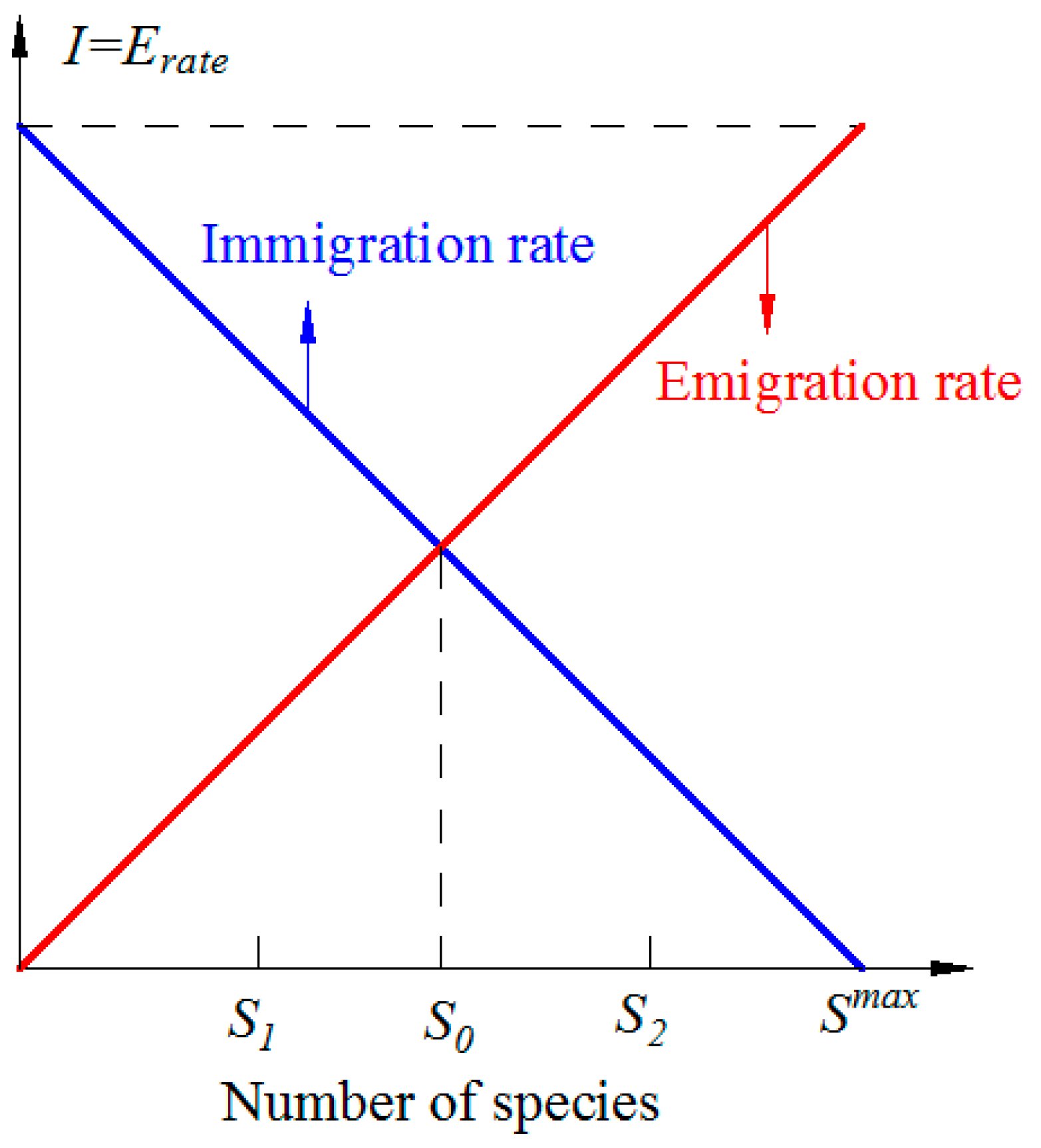
3.1. Basic Description of BBO

This paper presents an optimization algorithm based on the theory of biogeography, which is called biogeography-based optimization (BBO) [14]. Actually, BBO method has common features with other biology based optimization methods such as ABC, PSO, and GA but it has outstanding construction. The algorithm is found based on the observation of species emergence and migration from one island to the other. Based on that natural phenomenon, the mathematical model of biogeography is described [24,25].

Habitats are considered to be a good place with plentiful food, water sources, moderate temperature, proper humidity, and so on. The fact that different habitats have different conditions. Thus, each habitat is assigned to Habitat Suitability Index (HSI) for evaluating its quality level. The habitats which have difficult and harsh living conditions will be gotten a low index while other ones with better conditions will has higher index. Actually, the habitats with high HSI will attract many species for living and development and many species will emigrate to the habitats or nearby habitats for settling their life. The immigration rate is low and the emigration is high for habitats with high HSI vice versa. Because there are immigration and emigration in each habitat, thus there will be information exchange among considered habitats. The information about characteristics in each habitat is shared from this habitat to others through the migration operation of species. In the BBO, each design variable for particular population member is considered as suitability index variable (SIV) for that population member [14].

As shown in Figure 1, the number of species in a habitat is completely extinct when the maximum of immigration of species at rate I. Once the number of species (S_m) increases, the population density in the area increases. In this regard, there are fewer opportunities for new species to migrate to this habitat, causing low immigration rate. When such species achieve the largest population allowed to survive in this habitat, the immigration will come to zero and the emigration rate will reach a maximum [14].

The emigration and immigration rates are equal when the number of species is equal to S₀. This equilibrium point presents the balance between the immigration of the new species and the extinction of the old species [25]. In the BBO algorithm, there are two main operations: migration operation and mutation operation.

3.2. Migration Operation

This operation is a process of probabilistically modifying each individual in the habitat randomly. The habitat with high HSI tends to have a large number of species, high emigration rate, and immigration rate. A habitat with a high HSI tends to be more static in its species distribution. Immigration rate (${\lambda }_m$) and emigration rate (${\mu }_m$) are function of the number of species in a habitat and they are used to probabilistically share the information between habitats. For the habitat with no species, its immigration rate can be the highest. ${\lambda }_m$ and ${\mu }_m$ can be given by [26]:

$${\lambda }_m=I·(1-\frac{S_m}{S^{\max }})$$

(19)

$${\mu }_m=E·(\frac{S_m}{S^{\max }})$$

(20)

3.3. Mutation Operation

Mutation tends to increase the diversity of a species in a habitat. Due to natural events, the HSI of a habitat can change dramatically, causing the species count to shift away from its equilibrium value. Species count may be a probability value ($P_s$). If the probability P_m is very low, the considered solution will has more possibility to be newly updated. Therefore, the mutation rate of an individual solution can be calculated using species count probability, given by [27]:

$$m(s)=m^{\max }·(\frac{1-P_s}{P^{\max }})$$

(21)

3.4. Procedures for Implementing BBO Algorithm

The general implementation process of BBO algorithm for solving a typical optimization problem can be described briefly as follows [28]:

Step 1:

Initialize BBO parameters that are necessary for the algorithm. These parameters include population size (the number of habitats), maximum immigration rate, emigration rate, mutation coefficient, the elite keeping rate, the habitat modification probability, number of control variables.

Step 2:

Randomly generate population in the acceptable limits. Each member in the population contains the value of all the variations and every variation in the population indicates SIVs for that member.

Step 3:

Calculate and collect the value of objective function for all population members. This value indicates the HSI for that Habitat. In this case, if the problem is a constrained optimization problem, then a specific approach such as penalty is used for converting the constrained optimization problem into the unconstrained optimization problem.

Step 4:

Map the HSI value to obtain the species count. Here, the species count with high value is allotted to the population member having high HSI for maximization optimization problem.

Step 5:

Calculate immigration rate and emigration rate for H_m. Calculate λ_m and μ_m by using Equations (19) and (20), respectively.

Step 6:

Migration operation [29]. Migration operation is applied for modifying habitats, which are selected probabilistically (roulette wheel method can be used for selection). In this step, the selected habitat H_m,d will be replaced by another habitat H_j,d. While, the probability of election of H_m is proportional to immigration rate (λ_m) and the probability of election of H_j is proportional to emigration rate (μ_m).

$$H_{m,d}\leftarrow H_{j,d}$$

(22)

After applying migration operation, HSI must be calculated.

Step 7:

Mutation operator [29]. Mutation operation is applied for each selected habitat. Select H_m,_d according to mutation rate of Equation (21). The quantity of HSI for selected mutation habitat must be calculated again:

$$H_{m,d}\leftarrow H^{\min }+rand·(H^{\max }-H^{\min })$$

(23)

Step 8:

Best obtained solution is saved using elitism. Select population for next generation.

Step 9:

Repeat from step 3 until the specified number of generations or termination criterion is reached.

4. Biogeography-Based Optimization Algorithm for PVDG Units

With the strong growth in the connection of PVDG units in the distribution system, several methods have been employed to solve optimization problems considering the different objective functions and all constraints of distribution power networks. Actually, PVDG planning is one of the most important issues with significant impacts on economic and technical prospects. In this paper, PVDG units supply the active power directly to the loads in the radial distribution system with the presence of many nonlinear loads causing harmonics in the working systems. By installing and determining the optimal location as well as appropriate sizing of PVDG units, they can support the distribution power network with positive aspect. They can act as a power source supplying active power to load and playa very important electric component in reducing the total power loss, enhancing the voltage profile and maintaining the harmonic distortion falling into an accepted range. In this section, BBO is applied for determining the best location and the most appropriate rated power for PVDG units so that all total power loss is minimized while constraints regarding distribution power network and harmonic are exactly met. The implementation of BBO for the problem is described in detail as follows:

4.1. Producting Initial Solutions

Generation of initial population is an important step in implementation procedure of one method for solving an optimization problem. In the first task of the step, decision variables are chosen and included in each solution (i.e., each habitat of BBO method) and then generation of the whole population is easily done in the second task by setting all these decision variables to their predetermined range randomly. In the study, harmonic flow can be calculated by using forward/backward sweep technique (FW/BWST) but the technique needs information of location and rated active power of all installed PVDG units. Thus, the two factors including location and rated active power all PVDG units are considered to be decision variables in the problem and shown in Equation (24) below:

$$H_m=\left[L_{1m},P_{1m},\dots ,L_{jm},P_{jm},\dots ,L_{N_{DG}m},P_{N_{DG}m}\right];m=1,\dots ,N_{\mathrm{pop}}$$

(24)

Then, the whole population is randomly created within lower bound and upper bound as the following formula:

$$H_m=H^{\min }+rand·(H^{\max }-H^{\min });m=1,\dots ,N_{\mathrm{pop}}$$

(25)

where H^min and H^max are the lower bound and upper bound of all decision variables in each considered solution. The two important terms can be mathematically expressed by:

$$H^{\min }=\left[L_1^{\min },P_1^{\min },\dots ,L_j^{\min },P_j^{\min },\dots ,L_{N_{DG}}^{\min },P_{N_{DG}}^{\min }\right]$$

(26)

$$H^{\max }=\left[L_1^{\max },P_1^{\max },\dots ,L_j^{\max },P_j^{\max },\dots ,L_{N_{DG}}^{\max },P_{N_{DG}}^{\max }\right]$$

(27)

For all the study case with different systems such as 33-bus system and 69-bus system, the minimum location ($L_j^{\min }$) of the j^th PVDG unit, is bus No. 2 while the maximum location ($L_j^{\max }$) is equal to bus No. N_bus, the number of buses in the considered distribution power network. On the contrary to the range of location, predetermined range of rated power for each PVDG unit can be selected by operators. Basically, the minimum rated active power ($P_j^{\min }$) of the j^th PVDG unit is selected to be zero while its maximum ($P_j^{\min }$) is set to a value dependent on nominal voltage of the considered distribution system. The selection will be given and explained in simulation results section.

4.2. Produce New Solutions and Fix Violated Variables

BBO produces a new location and new size for all PVDG units by using migration operation as in step 6 and a mutation operation as in step 7 in the implementation procedures which were mentioned in Section 3 above. Normally, not every variable in a new solution violates predetermined bounds simultaneously but all variables in new solutions should be checked and fixed by using the following model:

$$H_m=\{\begin{array}{l}{H}^{\min }if{H}_m<H^{\min }\\ H^{\max }if{H}_m>H^{\max }\\ H_{m}else\end{array}$$

(28)

4.3. Calculate of Fitness Function Value

Performing initialization and new solution generation, all essential variables can be obtained and added into the data for running forward/backward sweep technique. Dependent variables yielded by the technique are current through all branches and voltage of all buses.

Total power loss can be obtained by using Equation (1) and objective function F₁ can be calculated by using Equation (2). Two terms regarding harmonics such as THD and IHD can be determined as a result of employing Equations (4) and (5), and then two terms in objective function F_{2_THD} and F_{2_IHD} are found by using Equations (6) and (7). Finally, F₂ is calculated by using Equation (10). The multi-objective function of the problem is obtained by using Equation (11). The multi-objective function and the violation of dependent variables are considered to be main terms in fitness function for judging quality of new solutions of BBO and other methods. The fitness function is constructed as follows:

$$F{F}_m=F_m+{\mu }_V{\displaystyle \sum _{i=1}^{N_{bus}}\Delta V_{i,m}^2}+{\mu }_I{\displaystyle \sum _{i=1}^{N_{br}}\Delta I_{n,m}^2}$$

(29)

where ∆V_i,m and ∆I_n,m can be yielded by the following formulas:

$$\Delta V_{i,m}=\{\begin{array}{ll}{V}_{i,m}-V_i^{\max }& if{V}_i>V_i^{\max }\\ V_i^{\min }-V_{i,m}& if{V}_{i,m}<V_i^{\min }\\ 0& else\end{array}$$

(30)

$$\Delta I_{n,m}=\{\begin{array}{ll}{I}_{n,m}-I_n^{\max }& if{I}_{n,m}>I_n^{\max }\\ 0& else\end{array}$$

(31)

4.4. Termination of Iterative Algorithm

The process of determining location and size of all installed PVDG units can be stopped based on comparison condition of current iteration and the predetermined maximum number of iterations. If current iteration is not equal to the maximum iteration, the search continues to be carried and otherwise, the search is stopped.

4.5. The Whole Search Procedure of BBO for Considered Problem

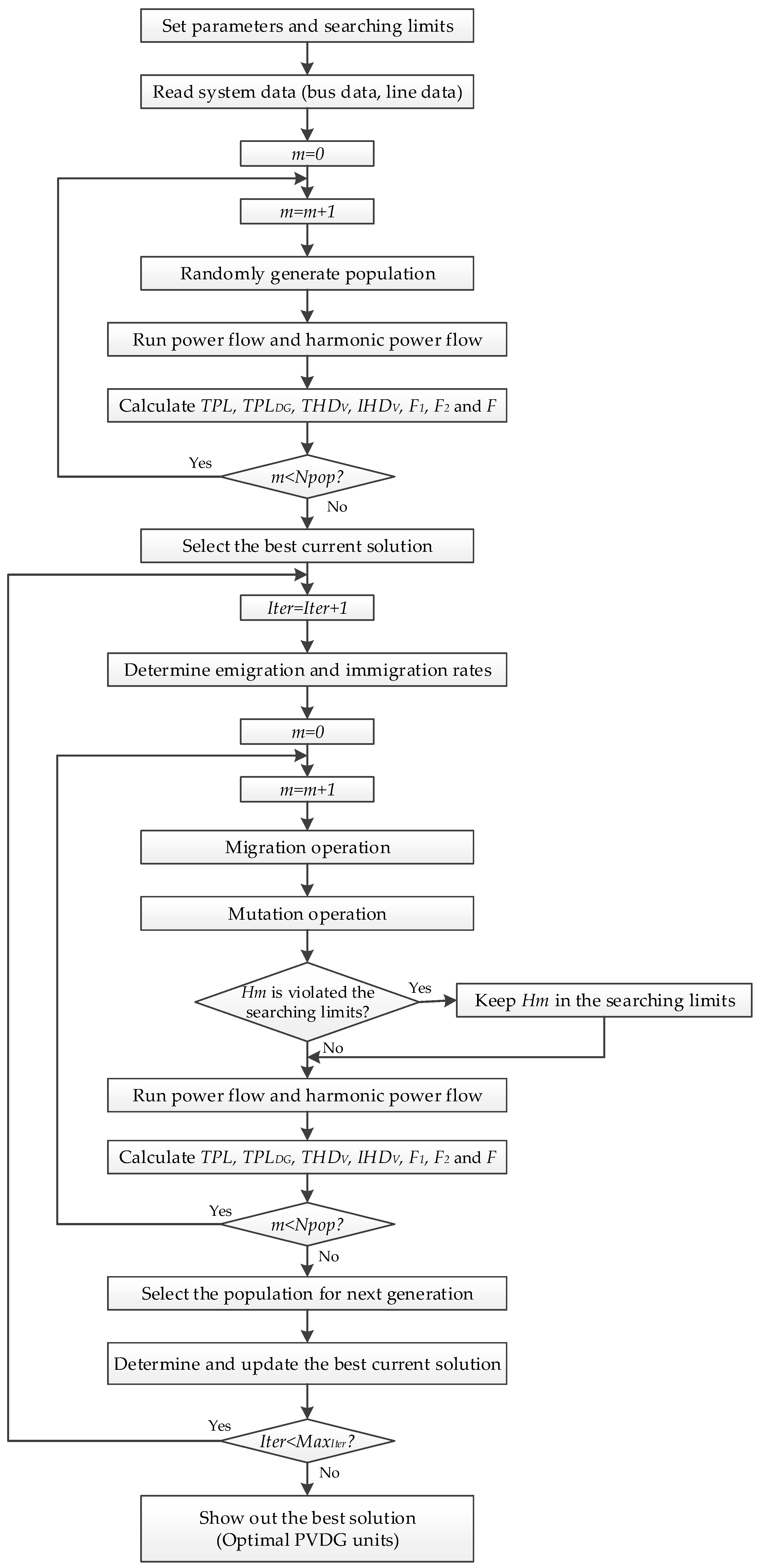
The whole computation process of using BBO for determining location and size of all installed PVDG units in distribution power network is given in Figure 2 and described in detail as follows:

Step 1:

Assign values to main parameters of BBO such as maximum immigration rate, emigration rate, mutation coefficient, kept population rate in percent, maximum number of iterations, population size, the number of installed PVDG units and rated power of each PVDG unit.

Step 2:

Read system data, which includes line data and bus data of the radial distributed system.

Step 3:

Generate population by using Equation (25).

Step 4:

Run power flow and harmonic power flow based on FW/BWTS to obtain all remaining variables I_n,m and V_i,m for the m^th solution.

Step 5:

Calculate total power loss and F₁ by using Equations (1) and (2)

Calculate THD and IHD by employing Equations (4) and (5)

Calculate F_{2_THD} and F_{2_IHD} by using Equations (6) and (7)

Determine F₂ by using Equation (10)

Calculate multi-objective function F by using Equation (11)

Evaluate quality of the solution m by calculating Equation (29).

Step 6: Select the best current solution based on the fitness values.

Step 7:

Set the computation to the first iteration (Iter = 1).

Step 8:

Determine the emigration rate and immigration rate for H_m by using Equations (19) and (20), respectively.

Step 9:

Migration operation: Follow the step 6 at procedures for implementing BBO algorithm.

Step 10:

Mutation operation: Follow the step 7 at procedures for implementing BBO algorithm.

Step 11:

Check limit violation for all new solutions and correct them by using Equation (28)

Step 12:

Run power flow and harmonic power flow based on FW/BWTS to obtain all remaining variables I_n,m and V_i,m for the m^th solution.

Step 13:

Calculate total power loss and F₁ by using Equations (1) and (2)

Calculate THD and IHD by employing Equations (4) and (5)

Calculate F_{2_THD} and F_{2_IHD} by using Equations (6) and (7)

Determine F₂ by using Equation (10)

Calculate multi objective function F by using Equation (11)

Evaluate quality of the m^th solution by calculating Equation (29).

Step 14:

Select the population for next generation by combining the top solution at previous generation with the top solution at current generation.

Step 15:

Determine and update the best current solution.

Step 16:

If Iter < Max_Iter, back to step 8. Otherwise, stop searching new solutions and report the best optimal solution.

5. Simulation Results

Here, we implement BBO method for finding optimal location and sizing of PVDG units with intent to reduce total active power loss while two main requirements such as harmonic flow constraints followed by IEEE Std. 519 and keeping voltage of all buses within an accepted range. Two study cases including an IEEE 33-bus distribution power network and an IEEE 69-bus distribution power network are chosen for running the BBO method. The data of the two systems are taken from [30,31] and given in the Appendix A. For verifying the performance of BBO, three other methods consisting of artificial bee colony (ABC), particle swarm optimization (PSO) with inertia weight and genetic algorithm (GA) are also executed for the two power systems. For each case, 30 trials of each method are run by coding in Matlab program language and personal computer with a 2.0 GHz CPU and 2.0 GB RAM.

For dealing with the multi-objective function (11), the weight factor ω₁ associated with total power loss objective is set to 0.6 while the weight factor ω₂ associated with the harmonic flow objective is set to 0.4. The selection can satisfy the constraint (12) and is also compatible with the contribution of each objective function to the multi objective function. In fact, although F₂ is the sum of two harmonic objective functions consisting of F_{2_THD} and F_{2_IHD}, the optimization of F₂ is not important as highly as F₁. We focus on minimizing total power loss F₁ and keeping THD and IHD within acceptable range as showing IEEE Std. 519.

In order to run BBO, the maximum immigration (I) and migration rates (E) for each habitat are fixed at 1; the maximum mutation rate (m_max) is set to 0.1; the habitat modification probability (P^mod) equal to 1; the combining ratio of selected habitat from the previous generation and current generation for next generation for each iteration is set to the range [20%–80%] (or the elite keeping rate equal to 0.2). For running GA, the optimal parameters are used as follows: the crossover probability (Cr) equal to 0.8 and mutation probability (Mu) equal to 0.001 [10]. To implement ABC, the colony size (employed bees + onlooker bees) is set to population size and the number of employed bees is equal to onlooker bees [32]. For running PSO, two acceleration factors c₁ and c₂ are set to 2 while the maximum and minimum inertia weight factor ω_max and ω_min are respectively fixed at 0.9 and 0.4 [33]. On the other hand, the same control parameters of the four methods including population size N_pop and the maximum number of iteration Max_Iter are selected to be 50 and 100, respectively.

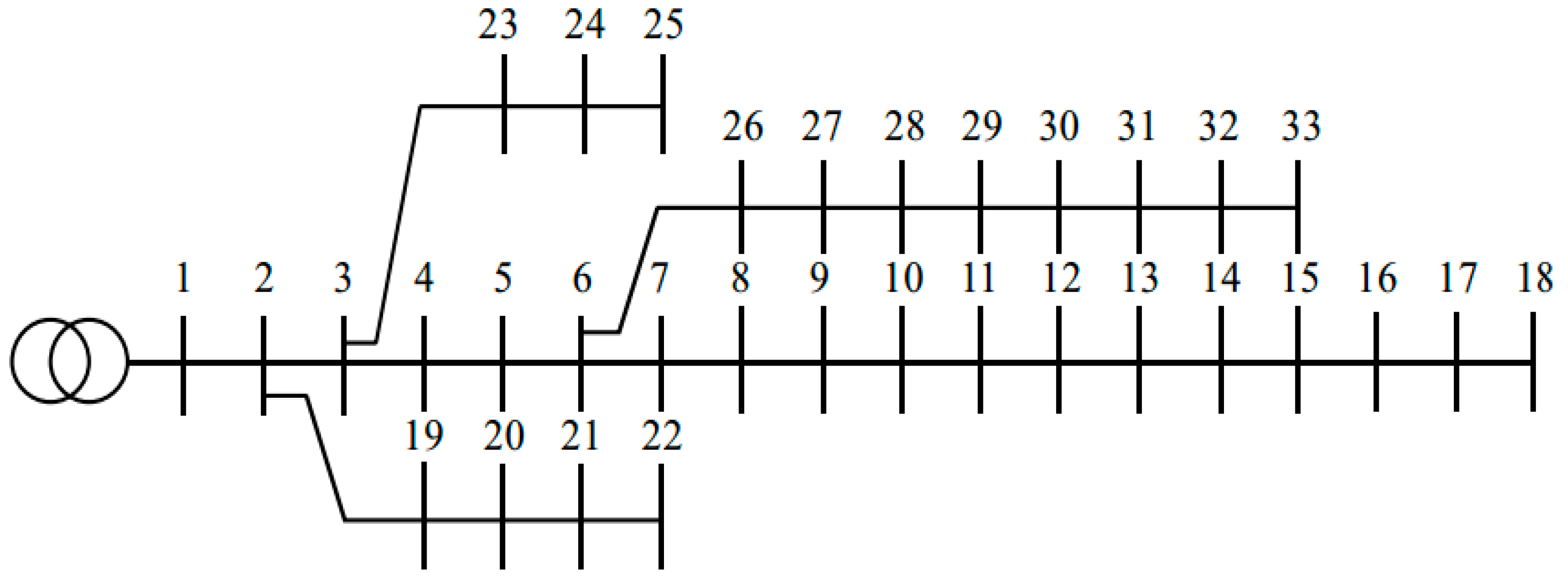
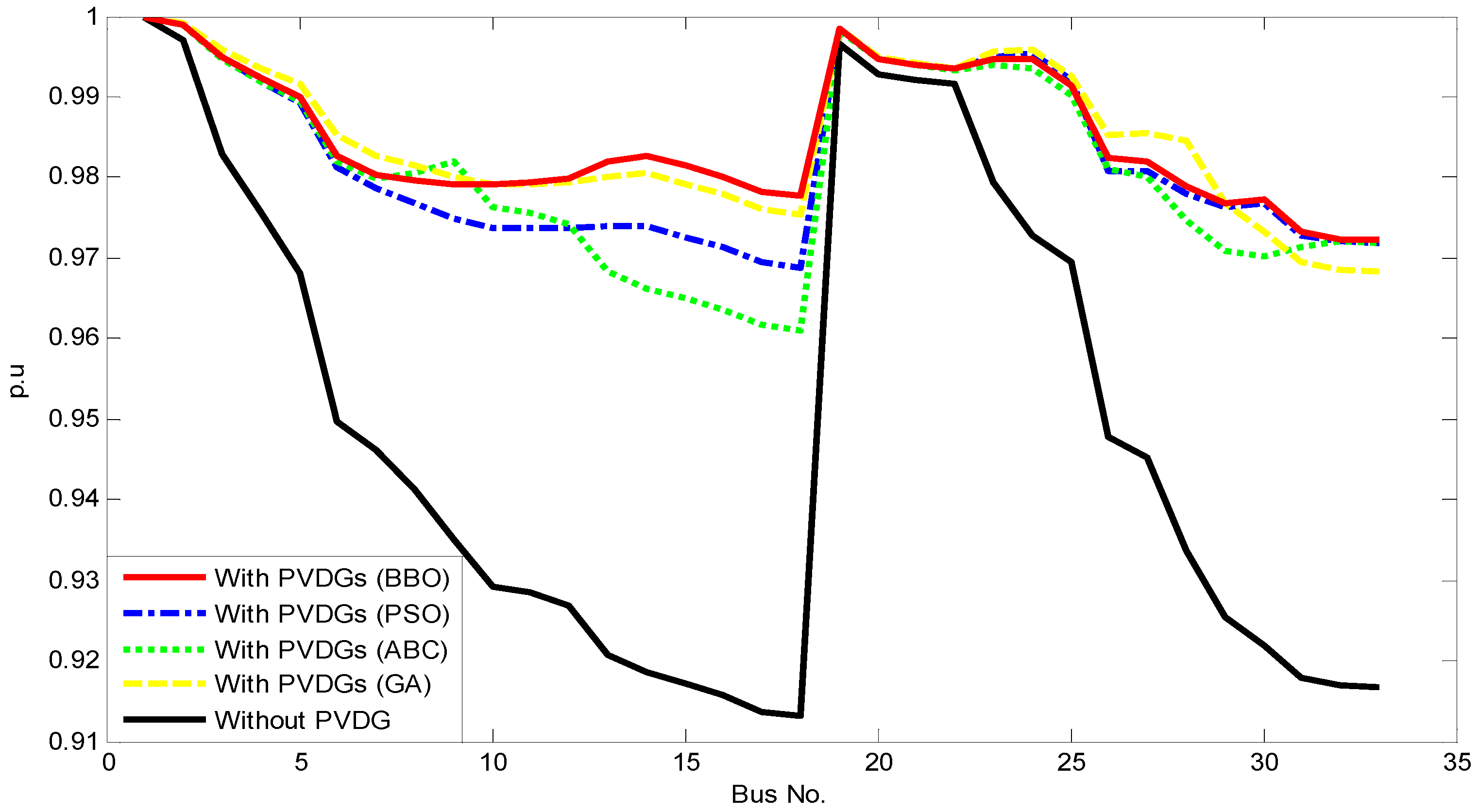
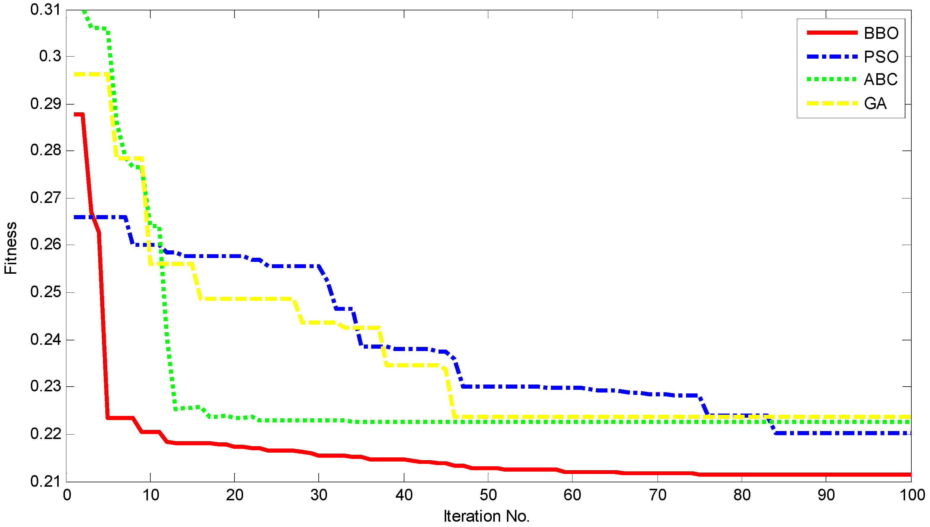
5.1. Case 1: IEEE 33-Bus Distribution Network

In this section, we install three different PVDG units in IEEE 33-bus system shown in Figure 3. The location and rated power of the units are control variables and need to be determined by using the four implemented methods. The locations that we can install the PVDG units are from bus 2 to bus 33 while the rated power of each PVDG unit can be selected to be from 0 MW and 2.0 MW [34]. In addition, for producing nonlinear loads, we inject five harmonic flows simultaneously to six loads located at buses 10, 15, 20, 24, 27 and 32. Information of the five harmonic flows such as order, magnitude as well as angle are taken from [35] and shown in

Table 1. Five harmonic flows injected to loads in distribution power networks.

Harmonic Order	Magnitude (%)	Angle (°)
5; 7; 11; 13; 17	0.765; 0.627; 0.248; 0.127; 0.071	28; −180; −59; 79; −253

.

The obtained numerical results for 30 trial runs consisting of the worst value of objective F, average value of F for 30 runs and the best value of obejctive F are reported in

Table 2. The comparison among four methods for IEEE 33-bus system.

Method	GA	ABC	PSO	BBO
The worst F	0.2570	0.2401	0.2523	0.2219
Average F	0.2375	0.2313	0.2291	0.2152
The best F	0.2238	0.2227	0.2203	0.2115
The best F1	0.3730	0.3712	0.3672	0.3525
The best F2	0	0	0	0

. In addition, two single objectives consisting of F₁ and F₂ corresponding to the best value of objective F are also reported in the table for better comparison. The best F values found by GA, ABC, PSO and BBO are 0.2238, 0.227, 0.2203 and 0.2115, respectively. According to these results, BBO can find less objective F than GA, ABC and PSO by 0.012, 0.011 and 0.009. In other words, BBO can improve the result over these methods up to 5.496%, 5.029% and 3.995%. The best F₂ equaling 0 from all methods indicates that the four methods can successfully reduce harmonic flows to acceptable value while the best F₁ regarding power loss found by BBO is the smallest equaling 0.3525 while that of GA, ABC and PSO is 0.3730, 0.3712 and 0.3672, respectively. The improvement of F₁ from BBO over GA, ABC and PSO is the same as the improvement of objective function F₁. For better comparisons of total power loss (which is considered in F₁) and harmonic flows (which are considered in F₂), we report $TH{D}_V^{\max }$, $IH{D}_V^{\max }$ and total power loss for the cases of uninstalling PVDG units and installing PVDG units by the four methods in

Table 3. The comparisons of IHD, THD and total power loss for IEEE 33-bus system.

Case	Without PVDG	With PVDGs and GA	With PVDGs and ABC	With PVDGs and PSO	With PVDGs and BBO
$TH{D}_V^{\max }$(%)	6.0331	4.1902	4.1627	4.2749	3.9355
$IH{D}_V^{\max }$(%)	3.9133	2.7187	2.7009	2.7736	2.5535
Total active power loss (MW)	0.2027	0.0756	0.0752	0.0744	0.0715

. It is obviously seen that before connecting PVDG units to grid, two harmonic components and total power loss are the highest. Namely, $TH{D}_V^{\max }$ and $IH{D}_V^{\max }$ are 6.0331% and 3.9133%, which are higher than required standard with 5% and 3%, respectively. Furthermore, the total power loss is very high, 0.2027 MW. However, after employing four methods in finding location and size of PVDG units in the system, both the two harmonic components and total power can significantly reduce. In fact, GA, ABC, PSO and BBO methods can reduce $TH{D}_V^{\max }$ and $IH{D}_V^{\max }$ to 4.1902% and 2.7187%, 4.1627% and 2.7009%, 4.2749% and 2.7736, and 3.9355% and 2.5535%, respectively. Clearly, these $TH{D}_V^{\max }$ and $IH{D}_V^{\max }$. are less than 5% and 3% as shown in IEEE Std. 519. Besides, the total power loss from four methods is also less than the case without installing PVDG units. The total power loss can be reduced to 0.0756 MW, 0.0752 MW, 0.0744 MW and 0.0715 MW for GA, ABC, PSO and BBO, respectively. The comparisons among the four applied methods recommend that BBO is the most appropriate method for installing PVDG units in the IEEE 33-bus system since it can support the power system in destroying harmonic flows and saving energy. Not only $TH{D}_V^{\max }$ and $IH{D}_V^{\max }$ but also total power loss from BBO are less than that from GA, ABC and PSO. Optimal solutions including location and size of each PVDG unit together with the total rated power of all units found by the four methods are reported in

Table 4. The best solution obtained by four methods for IEEE 33-bus system.

Method	The Best Solution	Total Capacity of PVDG Units
GA	Bus: 14–Size: 0.6947 MW	3.3419 MW
	Bus: 24–Size: 1.1844 MW
	Bus: 28–Size: 1.4628 MW
ABC	Bus: 09–Size: 1.1372 MW	3.0077 MW
	Bus: 24–Size: 1.0674 MW
	Bus: 32–Size: 0.8031 MW
PSO	Bus: 09–Size: 1.0625 MW	3.0590 MW
	Bus: 24–Size: 1.0447 MW
	Bus: 30–Size: 0.9518 MW
BBO	Bus: 14–Size: 0.7539 MW	2.9247 MW
	Bus: 24–Size: 1.0994 MW
	Bus: 30–Size: 1.0714 MW

. The total capacity of three optimal PVDG units that GA, ABC, PSO and BBO select are 3.3419 MW, 3.0077 MW, 3.0590 MW and 2.9247 MW, respectively. Compared to GA, ABC and PSO, BBO uses the smallest capacity of PVDG units while total power loss is the smallest. This result can indicate that it should install thee PVDG units at bus 14, bus 24 and bus 30 rather than other selections from the three compared methods.

The voltage profile of the IEEE 33-bus system for the cases of uninstalling and installing PVDG units by the four applied methods is shown in Figure 4. The five different curves point out that approximately all buses in the case without using PVDG units have lower voltage than other remaining cases. In addition, many buses in power system without PVDG units own voltage less than 0.95 pu, especially, two buses with less than 0.92 pu while those from power system using PVDG units are higher than 0.96 pu. Although the allowed range of voltage is [0.95, 1.05], higher voltage than lower bound is also preferred. Among the four applied methods, the lowest voltage from BBO is the best one with 0.9722 pu whilst that from PSO, ABC and GA are 0.9688 pu, 0.9611 pu and 0.9682 pu, respectively. Clearly, BBO is the most effective in improving voltage profile for the IEEE 33-bus system.

One more time, the outstanding performance of BBO can be demonstrated via the review on fitness functions obtained in 100 iterations for the best run shown in Figure 5. Solution of BBO at the 13th iteration can get better quality than that of three other methods at the final iteration. Furthermore, the improvement of solution quality of BBO can be seen clearly from the 13th iteration to the last one while other methods may be fallen into local zone and jumping out the zone seems not to be done.

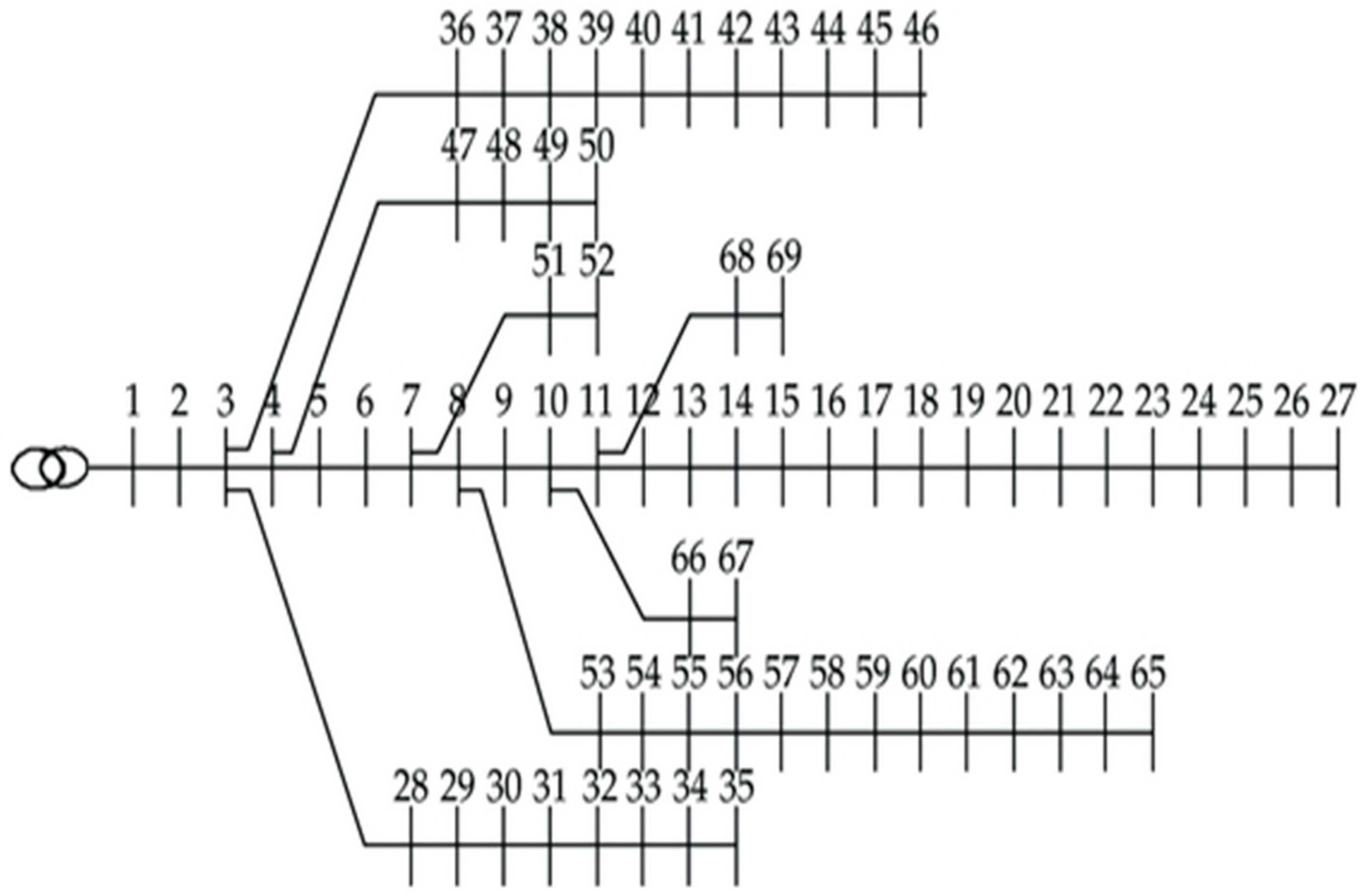
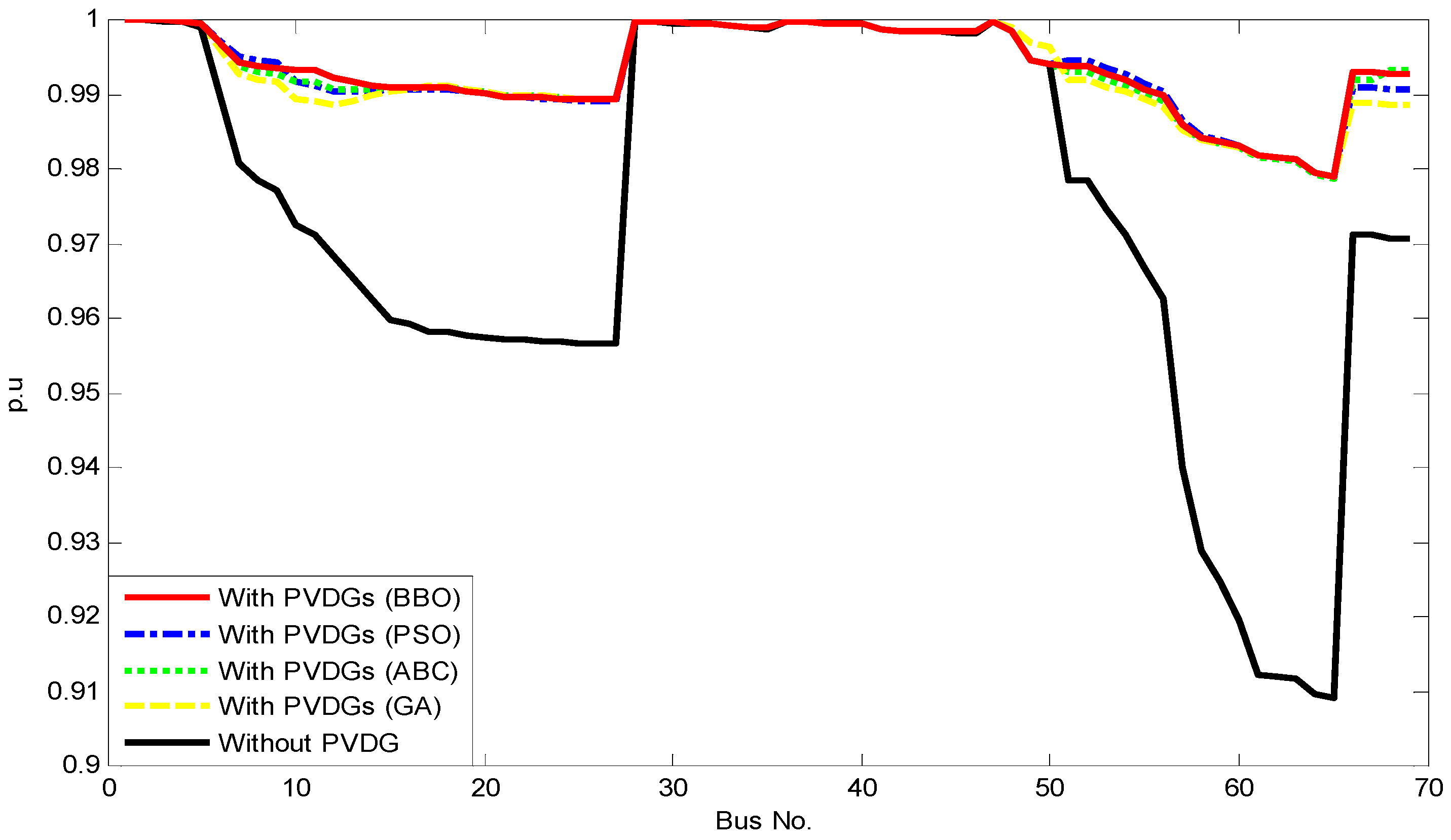
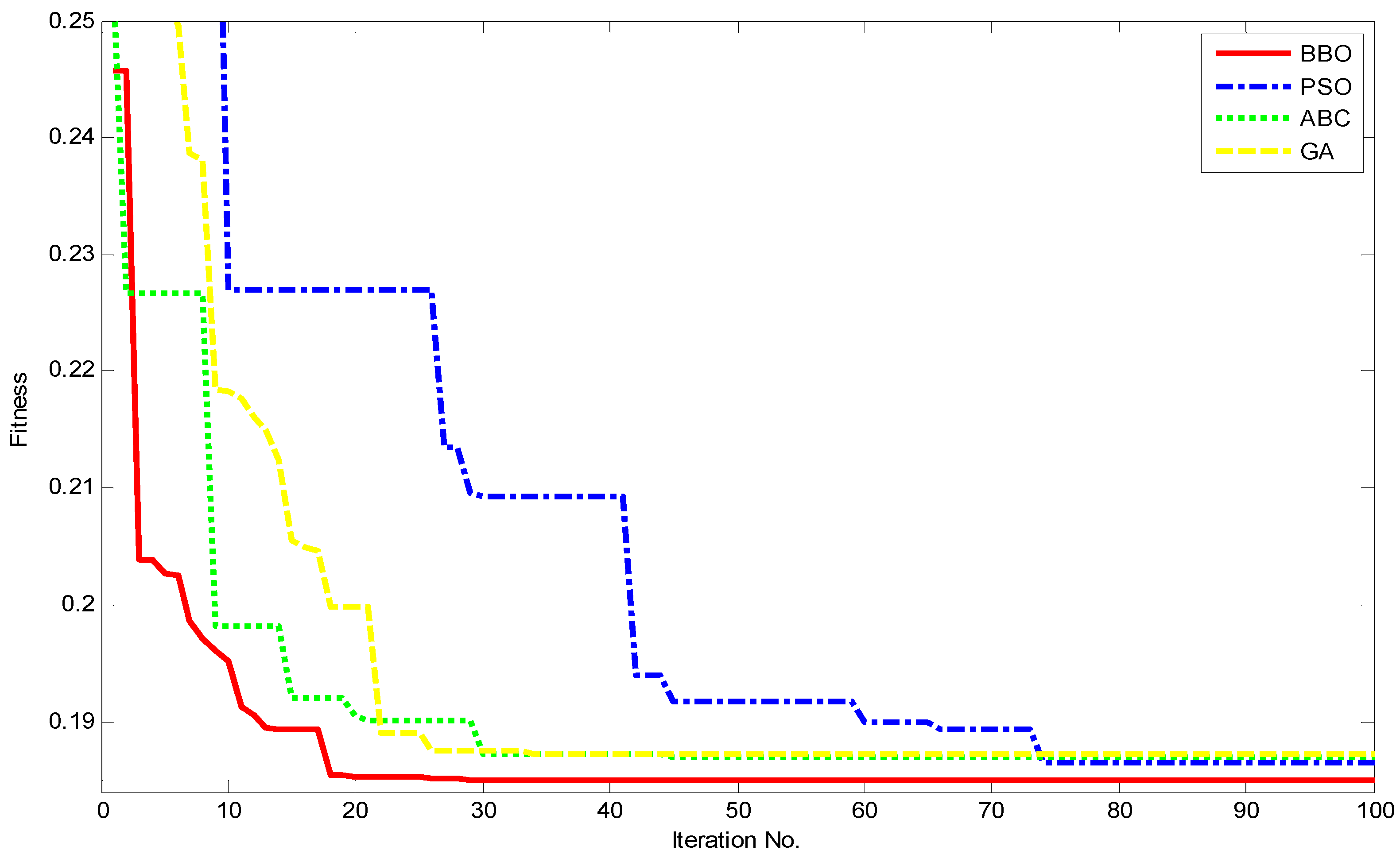
5.2. Case 2: IEEE 69-Bus Distribution Network

In this section, three different PVDG units are installed in the IEEE 69-bus system shown in Figure 6. Their locations as well as their rated power are determined by using the four implemented methods. Similar to IEEE 33-bus system, from bus 2 to bus 69 can be chosen for installing these units and the highest rated power of each PVDG unit is 2.0 MW. In addition, the five harmonic flows shown in Table 1 are simultaneously injected to eight buses in the system including 10, 12, 18, 19, 22, 25, 46 and 65.

Thirty trial runs are run for each of the four applied methods and three important values consisting of the best, average and worst objective functions are reported in

Table 5. The comparison of results obtained by four methods for IEEE 69-bus system.

Method	GA	ABC	PSO	BBO
The worst F	0.2499	0.1931	0.1955	0.1871
Average F	0.1902	0.1892	0.1881	0.1859
The best F	0.1873	0.1870	0.1864	0.1850
The best F1	0.3122	0.3117	0.3107	0.3083
The best F2	0	0	0	0

. The comparison of the best objective function F can lead to the evaluation that BBO can find the best optimal solution with the lowest objective among four methods once its value is 0.1850 while those from GA, ABC and PSO are 0.1873, 0.1870 and 0.1864, respectively. For the best F, the improvement of BBO over GA, ABC and PSO is 1.228%, 1.070% and 0.751%. Besides, the stablization in search process of BBO is also judged to be better than GA, ABC and PSO via the the best average of 0.1859 meanwhile that of three other methods is 0.1902, 0.1892 and 0.1881. Furthermore, the search ability fluctuation of the four methods can be reflected via the comparison of the worst solution. The worst solution of BBO is also the smallest among those of the four methods. Corresponding to the best objective function F, the best F₁ and the best F₂ are also reported in Table 5 for comparison of total power loss and harmonic flows. The four methods have the same F₂ equaling zero while F₁ of BBO is also the best one. Clearly, all the methods can reduce harmonic flows fallen into the allowed range less than 5% for THD and 3% for IHD from IEEE Std. 519. However, better comparison of harmonic objective function can be solved based on THD and IHD reported in

Table 6. The comparisons of IHD, THD and total power loss for IEEE 69-bus system.

Case	Without PVDG	With PVDGs and GA	With PVDGs and ABC	With PVDGs and PSO	With PVDGs and BBO
$TH{D}_V^{\max }$(%)	5.3964	3.7720	3.9330	3.3511	3.3037
$IH{D}_V^{\max }$(%)	3.4878	2.4372	2.5414	2.1619	2.1305
Total active power loss (MW)	0.2245	0.0701	0.0700	0.0698	0.0692

. Also, the exact total power loss can be observed in the table. As seen from the case without PVDG units, $TH{D}_V^{\max }$ and $IH{D}_V^{\max }$ are equal to 5.3964% and 3.4878%, which are higher than harmonic standard, 5 % and 3 %, respectively. On the contrary, those from four methods are less than 5% and 3% for $TH{D}_V^{\max }$ and $IH{D}_V^{\max }$, especially BBO with the best results, 3.3037% for $TH{D}_V^{\max }$ and 2.1305% for $IH{D}_V^{\max }$. Although GA, ABC and PSO can satisfy harmonic constraints, their results are worse than that of BBO. The power loss report also leads to the conclusion that the power system is working ineffectively due to the highest power loss for the case without PVDG units installed, but the power loss can be optimized when applying BBO for determining location and capacity of PVDG units. The total power loss significantly reduces from 0.2245 MW to 0.0692 MW corresponding to without PVDG units and with PVDG units from BBO’s solution. Clearly, the instalation of PVDG untis is really important and the effectiveness of BBO is trully confirmed.

Bus numbers where PVDG units are being installed and the capacity of the PVDG units together with the total capacity of all units found by the four methods are summarized in

Table 7. The best solutions and the total capacity of PVDG untis found by the four implemented methods for IEEE 69-bus system.

Method	The Best Solution	Total Capacity of PVDG Units
GA	Bus: 18–Size: 0.5239 MW	3.2451 MW
	Bus: 49–Size: 0.9356 MW
	Bus: 61–Size: 1.7856 MW
ABC	Bus: 18–Size: 0.4290 MW	2.5015 MW
	Bus: 61–Size: 1.7405 MW
	Bus: 69–Size: 0.3320 MW
PSO	Bus: 09–Size: 0.6385 MW	2.7678 MW
	Bus: 17–Size: 0.4390 MW
	Bus: 61–Size: 1.6903 MW
BBO	Bus: 11–Size: 0.5388 MW	2.6241 MW
	Bus: 18–Size: 0.3669 MW
	Bus: 61–Size: 1.7184 MW

. The total capacities of three proposed PVDG units obtained by GA, ABC, PSO and BBO methods are 3.2451 MW, 2.5015 MW, 2.7678 MW and 2.6241 MW, respectively. It is clear that BBO can find signficantly and slightly less capacity than GA and PSO but it is slighly higher than ABC. Nevertheless, the effectiveness of BBO in terms of total power loss minimization and harmonic flow reduction is superior to ABC for the system.

The voltages of all buses in the IEEE 69-bus system for the case without PVDG units and for four cases with PVDG units from GA, ABC, PSO and BBO are illustrated in Figure 7. There are five voltage magnitude values at each bus in the figure for the comparison of voltage improvement. All the curves see that voltage of the case without PVDG unit is always below that of four other cases. Especially, the lowest voltage of the system without PVDG is equal to 0.9092 pu, but the lowest one from four other cases is much higher. They are 0.9810 pu, 0.9790 pu, 0.9789 pu and 0.9790 pu for BBO, PSO, ABC, GA, respectively. Clearly, BBO has better voltage magnitude than other methods. Furthermore, the curves can see that approximately all buses of BBO own better voltage than other ones.

One more time, the outstanding performance of BBO over GA, ABC and PSO can be observed via Figure 8. All solutions found by BBO are much more effective than those from other ones since the deviation from red curve and other curves is significant and clearly seen.

The BBO solution at the 18th iteration has lower fitness than solutions of three other methods at the final iteration. It is clear that BBO has faster search ability than other ones for the system with 69 buses. In summary, simulation results in Section 5 can lead to the two following main conclusions:

(1)

Installing PVDG units in a distribution power network can bring benefits such as destroying harmonic flows acceptably, improving voltage profiles, and reducing total power losses;

(2)

Among the four implemented methods, including GA, ABC, PSO and BBO, the most effective method for determining location and size of PVDG units in distribution power network is BBO. BBO can reduce harmonic magnitude harmfully influencing loads, improve voltage profile, reduce total power loss and minimize capacity of PVDG units.

6. Conclusions

In this paper, an effective biogeography-based optimization algorithm (BBO) has been employed to determine optimal location and size of PVDG units installed in two IEEE distribution network with 33 buses and 69 buses with intent to minimize power loss and satisfy IEEE Std. 519 related to harmonic flow limits. The multi objective function with the presence of total power loss and two harmonic components consisting of THD and IHD has been considered to be minimized for the two systems. In the study, we have proposed a very effective multi-objective function in which total power loss in MW has been considered in the first objective F₁ and the sum of THD and IHD has been considered in the second objective. In addition, objective F₁ and objective F₂ could be converted into the same per unit with the same range less than 1. By using the multi-objective function, the selection of weight factors associated with the two objectives has become a simple task due to a very small deviation between the two objectives. Furthermore, as using the multi-objective function, harmonic flow could be kept within allowed range and the total power loss minimization can be focused better. The results from IEEE 33-bus distribution network and IEEE 69-bus distribution network have indicated that harmonic flows could be treated in the case of installing PVDG units and total power loss could be reduced effectively. In addition, three other meta-heuristic algorithms have also been applied for optimizing location and size of PVDG units. The result comparisons related to the considered problem such as total power loss, THD, IHD, voltage profile and total capacity of all PVDG units as well as related to solution search ability of the four methods could show the outstanding performance of BBO over GA, ABC and PSO. As a result, it could lead to a conclusion that the installation of PVDG units is highly important in distribution power network for the case with harmonic flows, and the application of BBO brings high effectiveness.

References

1. Pandey, R.R.; Arora, S. Distributed generation system: A review and its impact on India. Int. Res. J. Eng. Technol. (IRJET) 2016, 3, 758–765. [Google Scholar]
2. Kamaruzzaman, A.Z.; Mohamed, A.; Shareef, H. Effect of grid-connected photovoltaic systems on static anddynamic voltage stability with analysis techniques—A review. Universiti Kebangsaan Malays. 2015, 134–138. [Google Scholar] [CrossRef]
3. Sahib, J.T.; Ghani, A.R.M.; Jano, Z.; Mohamed, H.I. Optimum allocation of distributed generation using PSO: IEEE test case studies evaluation. Int. J. Appl. Eng. Res. 2017, 12, 2900–2906. [Google Scholar]
4. Saad, M.N.; Sujod, Z.M.; Ming, H.L.; Abas, F.M.; Jadin, M.S.; Ishak, R.M.; Abdullah, H.R.N. Impacts of photovoltaic distributed generation location and size on distribution power system network. Int. J. Power Electron. Drive Syst. (IJPEDS). 2018, 9, 905–913. [Google Scholar]
5. Sadeghian, H.; Athari, H.M.; Wang, Z. Optimized solar photovoltaic generation in a real local distribution network. In Proceedings of the 2017 IEEE Power & Energy Society Innovative Smart Grid Technologies Conference (ISGT), Washington, DC, USA, 23–26 April 2017; pp. 2472–8152. [Google Scholar]
6. Khorasany, M.; Aalami, H. Determination of the optimal location and sizing of DGs in radial distribution network using modified PSO and ABC algorithms. Int. J. Mod. Trends Eng. Res. 2016, 3, 429–436. [Google Scholar]
7. Kumawat, A.; Singh, P. Optimal placement of capacitor and DG for minimization of power loss using genetic algorithm and artificial bee colony algorithm. Int. Res. J. Eng. Technol. (IRJET) 2016, 3, 2482–2488. [Google Scholar]
8. Phuangpornpitak, W.; Bhumkittipich, K. Optimal placement and sizing of distributed generation for power loss reduction using particle swarm optimization. Res. J. Appl. Sci. Eng. Technol. 2014, 7, 1211–1216. [Google Scholar] [CrossRef]
9. Sedighizadeh, M.; Rezazadeh, A. Using genetic algorithm for distributed generation allocation to reduce losses and improve voltage profile. Int. Sch. Sci. Res. Innov. 2008, 2, 50–55. [Google Scholar]
10. Sulistyowati, R.; Rianwan, C.D.; Ashari, M. PV farm placement and sizing using GA for area development plan of distribution network. In Proceedings of the 2016 International Seminar on Intelligent Technology and Its Application, Lombok, Indonesia, 28–30 July 2016. [Google Scholar] [CrossRef]
11. Othman, M.M.; El-Khattam, W.; Hegazy, G.Y.; Abdelaziz, Y.A. Optimal placement and sizing of distributed generators in unbalanced distribution systems using supervised big bang-big crunch method. IEEE Trans. Power Syst. 2014, 30, 911–919. [Google Scholar] [CrossRef]
12. Ameli, A.; Bahrami, S.; Khazaeli, F.; Haghifam, M. A multiobjective particle swarm optimization for sizing and placement of DGs from DG owner’s and distribution company’s viewpoints. IEEE Trans. Power Deliv. 2014, 29, 1831–1840. [Google Scholar] [CrossRef]
13. Umar; Firdaus; Ashari, M.; Penangsang, O. Optimal location, size and type of DGs to reduce power loss and voltage deviation considering THD in radial unbalanced distribution systems. In Proceedings of the 2016 International Seminar on Intelligent Technology and Its Application (ISITIA), Lombok, Indonesia, 28–30 July 2016; Volume 29, pp. 1831–1840. [Google Scholar] [CrossRef]
14. Simon, D. Biogeography-based optimization. IEEE Trans. Evolut. Comput. 2008, 12, 702–713. [Google Scholar] [CrossRef]
15. Kadir, A.F.A.; Mohamed, A.; Shareef, H.; Wanik, C.Z.M.; Ibrahim, A.A. Optimal sizing and placement of distributed generation in distribution system considering losses and THDv using gravitational search algorithm. Przegląd Elektrotechniczny 2013, 89, 132–136. [Google Scholar]
16. Teng, H.J.; Chang, Y.C. Backward/Forward sweep-based harmonic analysis method for distribution system. IEEE Trans. Power Deliv. 2007, 22, 1665–1672. [Google Scholar] [CrossRef]
17. Beránek, V.; Olšan, T.; Libra, M.; Poulek, V.; Sedláček, J.; Dang, M.-Q.; Tyukhov, I.I. New Monitoring System for Photovoltaic Power Plants’ Management. Energies 2018, 11, 2495. [Google Scholar] [CrossRef]
18. Allah, A.B.; Djamel, L. Control of power and voltage of solar grid connected. Int. J. Electr. Comput. Eng. (IJECE) 2016, 6, 26–33. [Google Scholar] [CrossRef]
19. Hu, H.; Shi, Q.; He, Z.; He, J.; Gao, S. Potential harmonic resonance impact of PV inverter filters on distribution systems. IEEE Trans. Sustain. Energy 2015, 6, 151–161. [Google Scholar] [CrossRef]
20. Sariraja, R.M.; Muthulakshmi, K.; Kumar, S.V.; Abinaya, T. PSO based optimal distributed generation placement and capacity by considering harmonic limits. Tech. Gaz. 2017, 24, 391–398. [Google Scholar]
21. Prakash, P.; Khatod, K.D. Optimal sizing and siting techniques for distributed generation in distribution system: A review. Renew. Sustain. Energy Rev. 2016, 111–130. [Google Scholar] [CrossRef]
22. Wazir, A.; Arbab, N. Analysis and optimization of IEEE 33 bus radial distributed system using optimization algorithm. J. Eng. Trends Appl. Eng. 2016, 1, 17–21. [Google Scholar]
23. Rao, R.V.V.P.; Raju, S.S. Voltage regulator placement in radial distribution system using plant growth simulation algorithm. Int. J. Eng. Sci. Technol. 2010, 2, 207–217. [Google Scholar] [CrossRef]
24. Lim, L.W.; Wibowo, A.; Desa, I.M.; Haron, H. A Biogeography-based optimization algorithm hybridized with tabu search for the quadratic assignment problem. Comput. Intell. Neurosci. 2016. [Google Scholar] [CrossRef] [PubMed]
25. Sadeghi, H.; Ghaffarzadeh, N. A simultaneous biogeography based optimal location of DG units and capacitor bank in distribution systems with nonlinear loads. J. Electr. Eng. 2016, 67, 351–357. [Google Scholar] [CrossRef]
26. Kumar, R.A.; Premalatha, L. Optimal power flow for a deregulated power system using adaptive real coded biogeography-based optimization. Electr. Power Energy Syst. 2015, 73, 393–399. [Google Scholar] [CrossRef]
27. Wang, Z.; Liu, P.; Ren, M.; Yang, Y.; Tian, X. Improved biogeography-based optimization based on affinity propagation. Int. J. Geo-Inf. 2016, 5, 129. [Google Scholar] [CrossRef]
28. Rao, R.V.; Savsani, V.J. Chapter 2: Advanced optimization techniques. Mech. Des. Opt. Using Adv. Opt. Tech. 2012, 7, 11–14. [Google Scholar]
29. Wang, C.Z.; Wu, B.X. Hybrid biogeography-based optimization for integer programming. Sci. World J. 2014, 2014, 672983. [Google Scholar] [CrossRef]
30. Palomino, G.G.; Barragán, A.A.L.; Trujillo, R.E. Locating distributed generation units radial systems. Contemp. Eng. Sci. 2017, 10, 1035–1046. [Google Scholar] [CrossRef]
31. Aman, M.M.; Jasmon, B.G.; Bakar, A.H.A.; Mokhlis, H. A new approach for optimum simultaneous multi-DG distributed generation Units placement and sizing based on maximization of system load ability using HPSO (hybrid particle swarm optimization) algorithm. Energy 2014, 66, 202–215. [Google Scholar] [CrossRef]
32. Sajeevan, S.; Padmavathy, N. Optimal allocation and sizing of distributed generation using artificial bee colony algorithm. Int. Res. J. Eng. Technol. (IRJET) 2016, 3, 1244–1252. [Google Scholar]
33. Pandey, D.; Bhadoriya, S.J. Optimal placement & sizing of distributed generation (DG) to minimize active power loss using particle swarm optimization (PSO). Int. J. Sci. Technol. Res. 2014, 3, 246–254. [Google Scholar]
34. Vita, V. Development of a decision-making algorithm for the optimum size and placement of distributed generation units in distribution networks. Energies 2017, 10, 1433. [Google Scholar] [CrossRef]
35. Harmonic Spectrum. Available online: https://github.com/tshort/OpenDSS/blob/master/Test/indmachtest/Spectrum.DSS (accessed on 7 January 2014).
Figure 1. The relationship between the number of species, emigration rate and immigration rate.
Energies 12 00174 g001
Figure 2. The flowchart of using BBO method for determining location and sizing of all installed PVDG units.
Energies 12 00174 g002
Figure 3. IEEE 33-bus distribution network.
Energies 12 00174 g003
Figure 4. Voltage profile without and with PVDG units.
Energies 12 00174 g004
Figure 5. Convergence of implemented methods within 100 iterations.
Energies 12 00174 g005
Figure 6. IEEE 69-bus distribution network.
Energies 12 00174 g006
Figure 7. Volt profile without and with PVDG units.
Energies 12 00174 g007
Figure 8. Convergence of implemented methods in 100 iterations.
Energies 12 00174 g008