Evaluation of Direct Horizontal Irradiance in China Using a Physically-Based Model and Machine Learning Methods


1
School of Resource and Environmental Science, Wuhan University, Wuhan 430079, China
2
School of Geographic Sciences, Xinyang Normal University, Xinyang 464000, China
3
Laboratory of Critical Zone Evolution, School of Earth Sciences, China University of Geosciences, Wuhan 430074, China
*
Author to whom correspondence should be addressed.
Energies 2019, 12(1), 150; https://doi.org/10.3390/en12010150
Submission received: 19 November 2018
/
Revised: 18 December 2018
/
Accepted: 27 December 2018
/
Published: 2 January 2019
(This article belongs to the Special Issue Solar Thermal Energy Utilization Technologies in Buildings)
Abstract
:Accurate estimation of direct horizontal irradiance (DHI) is a prerequisite for the design and location of concentrated solar power thermal systems. Previous studies have shown that DHI observation stations are too sparsely distributed to meet requirements, as a result of the high construction and maintenance costs of observation platforms. Satellite retrieval and reanalysis have been widely used for estimating DHI, but their accuracy needs to be further improved. In addition, numerous modelling techniques have been used for this purpose worldwide. In this study, we apply five machine learning methods: back propagation neural networks (BP), general regression neural networks (GRNN), genetic algorithm (Genetic), M5 model tree (M5Tree), multivariate adaptive regression splines (MARS); and a physically based model, Yang’s hybrid model (YHM). Daily meteorological variables, including air temperature (T), relative humidity (RH), surface pressure (SP), and sunshine duration (SD) were obtained from 839 China Meteorological Administration (CMA) stations in different climatic zones across China and were used as data inputs for the six models. DHI observations at 16 CMA radiation stations were used to validate their accuracy. The results indicate that the capability of M5Tree was superior to BP, GRNN, Genetic, MARS and YHM, with the lowest values of daily root mean square (RMSE) of 1.989 MJ m−2day−1, and the highest correlation coefficient (R = 0.956), respectively. Then, monthly and annual mean DHI during 1960–2016 were calculated to reveal the spatiotemporal variation of DHI across China, using daily meteorological data based on the M5tree model. The results indicated a significantly decreasing trend with a rate of −0.019 MJ m−2during 1960–2016, and the monthly and annual DHI values of the Tibetan Plateau are the highest, while whereas the lowest values occur in the southeastern part of the Yunnan−Guizhou Plateau, the Sichuan Basin and most of the southern Yangtze River Basin. The possible causes for spatiotemporal variation of DHI across China were investigated by discussing cloud and aerosol loading.
1. Introduction
Solar energy is regarded as a clean, renewable, sustainable and environmentally-friendly energy source for life on Earth [1]. With the rapid economic development of China, large amounts of fossil fuel have been burned in recent decades, which have caused serious environmental pollution [2]. Moreover, the concentration of atmospheric greenhouse gases continues to increase unless the global consumption of fossil fuel drops sharply [3]. To address the problem of air pollution, solar electrical energy applications converting solar energy into heat and electricity have been developed rapidly in China in recent years. For example, since 2016, China has had the largest solar power generation capability, with an installed capacity of 77.42 GW [4]. Therefore, an accurate estimation of solar radiation is crucial for site resource analysis, system design and plant operation [5].
Solar radiation consists of two parts: direct radiation and diffuse radiation, which determine areas with potential for solar power generation, and thus have a profound influence on the solar photovoltaic (PV) industry [6]. There are two main types of solar energy systems: concentrated solar power thermal systems (CSP) and photovoltaic (PV) systems, which use the direct radiation and both the direct and diffuse components (global radiation), respectively. Currently, solar radiation is measured mainly using four methods: solar radiation retrieval from satellite observations, reanalysis data, simulations based on general circulation models, and direct measurements at the surface [7]. Several surface-radiation measurement networks have been established worldwide; for example the Baseline Surface Radiation Network (BSRN), which provides measurements of global radiation of high accuracy and high-temporal resolution [8]; and the Global Energy Balance Archive (GEBA), which compiles monthly global radiation data from more than 2500 stations worldwide [9]. However, because of their sparse and heterogeneous distribution, these networks are insufficient for deriving estimates of global radiation (including direct radiation) from surface observations alone. Remote sensing provides an alternative method for retrieving spatiotemporally continuous solar radiation values; for example, the Global Energy and Water Cycle Experiment-Surface Radiation Budget (GEWEX-SRB) provides solar radiation products at a 3h temporal resolution and 1° spatial resolution [10,11], as does the International Satellite Cloud Climatology Project-Flux Data (ISCCP-FD) at 3h intervals and 2.5° spatial resolution [12]. However, they are limited because of the relatively short historical record, and in addition, their accuracy needs further improvement. Reanalysis datasets are another feasible means of producing global radiation products and have a relatively high temporal resolution. For example, the National Center for Environmental Prediction−National Centre for Atmospheric Research (NCEP−NCAR) reanalysis is a global reanalysis from 1948 to near-present, with a temporal resolution of 6 h and spatial resolution of 1.9° [13,14]; in addition, the Japan Meteorological Agency (JMA) conducted the second Japanese global atmospheric reanalysis, called the Japanese 55-year reanalysis or JRA-55, which covers the period from 1958 to 2013, and has a 3h temporal resolution and spatial resolution of 0.56° [15]. Unfortunately, however, in comparison with ground measurements, there is a larger positive bias in current reanalysis products [16]. Furthermore, all the three above-mentioned sources mainly provide global radiation estimates and there is a lack of products for direct radiation. However, direct radiation has great potential for the application of CSP electricity production across China and, therefore, it is of vital importance to develop models to estimate and map direct radiation to maximize the efficiency of installations of solar power plants using CSP.
Many methods have been developed to estimate solar radiation [17,18,19,20,21], and they can be divided into three principal categories: empirical parameterization models, physical models and data-driven models [22]. Empirical parameterization schemes are designed to indirectly estimate solar radiation from routine meteorological variables (mainly temperature, sunshine duration and cloud data) [23,24,25,26,27,28,29]. For example, Yao [30] proposed a new high-quality sunshine duration model to estimate daily global solar radiation, and the results were shown to be more accurate than those of the Lewis model. In addition, Hassan [31] proposed 20 different ambient temperature-based models for estimating the monthly average daily global solar radiation; the performance of 12 of the new models was superior to that of the three models selected from the literature. However, because no physical principles were considered explicitly in these estimation schemes, the calibration parameters often vary between sites, which limits the general applicability of the models, and may lead to large uncertainties in solar radiation estimates at uncalibrated sites. Physical models provide an effective means of estimating solar radiation with high accuracy; for example, a clear-sky broadband radiative transfer model was developed by Yang [32,33], which was shown to be one of the best broadband models in terms of accuracy and robustness. In addition, Qin [7] developed an efficient physically-based parameterization scheme to derive surface solar irradiance in China and the USA; the results showed that the model can effectively retrieve surface solar irradiance, with a root mean square error (RMSE) of 35 Wm−2, on a daily basis. In comparison, data-driven models are more concise in that they do not explicitly incorporate physical principles and do not require prior assumptions about the underlying data. In other examples, Deo and Sahin [22] forecast solar radiation using an ANN model in Queensland. Celik [34] optimized the performance of an ANN model to provide an efficient estimation of solar radiation for the eastern Mediterranean region of Turkey.
However, most studies estimating solar radiation have focused on global radiation, and few on estimating direct radiation [35]. Nevertheless, there has been some success in estimating direct radiation worldwide using various methods. For example, Bertrand [36] evaluated decomposition models of varying degrees of complexity to estimate direct solar irradiance from Meteosat second generation images over Belgium; Rosales [37] proposed an analytical and numerical model to simulate the interactions of direct solar radiation. Gueymard [38,39] compared four models (CPCR2, MLWT2, REST and Yang) and concluded that the newly developed MLWT2 model provides the best performance in all direct solar radiation estimation tests. Mellit et al. [5] developed an adaptive model for predicting hourly DHI and a good agreement between measured and predicted data was obtained. However, there are very few published studies about the estimation of direct radiation in China. Although Chen et al [40] developed twenty satellite-based MOD08-M3 atmospheric product and proposed the best site-specific models for DHI in China; Tang [35] made the first attempt to construct direct solar radiation data sets for China based on a physical model. It is necessary to apply and compare different modeling techniques for the simulation of direct radiation. In addition, there have been very few studies focusing on the analysis and comparison of the patterns of variation within different climatic zones.
From the above, it can be concluded that there is an increasing need for accurate and reliable daily direct radiation data for solar energy applications using various methods within different climatic zones in China. Therefore, we conducted a comparative study of the spatiotemporal performance of six selected direct radiation models in different climate zones of China. The model with the highest degree of accuracy was used to demonstrate the temporal variation of annual and monthly mean direct radiation, and the spatial distribution of annual mean sum of potential CSP electricity production in different climatic zones across China. Our study is the first assessment of various direct radiation models in different ecosystems in China.
2. Materials and Methods
2.1. Sites and Data
2.1.1. Observation Data
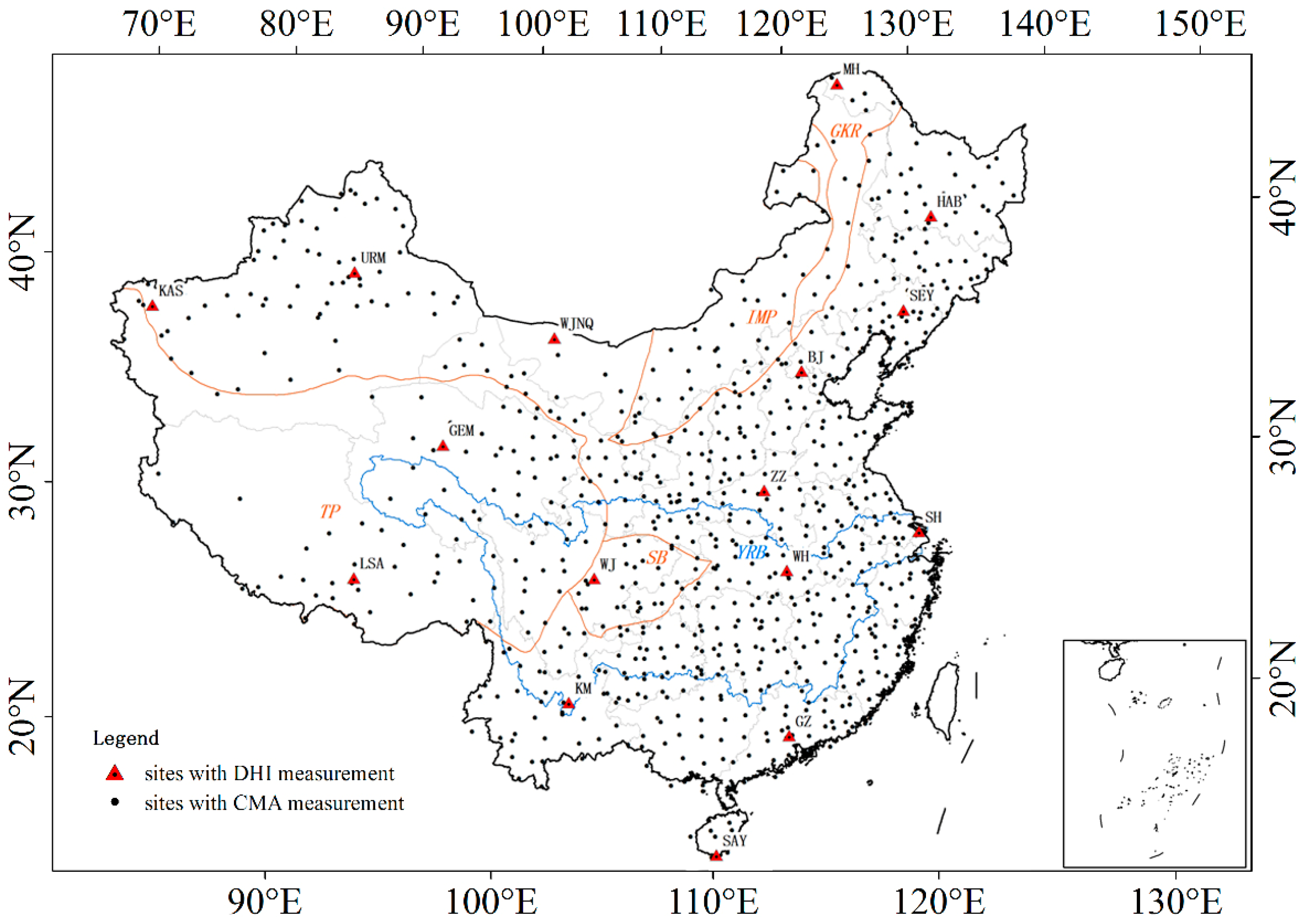
Figure 1 shows the location of 16 DHI stations and 839 CMA stations across China. Daily meteorological measurements of 839 CMA stations were used to estimate DHI values. The meteorological elements of these measurements were sunshine duration (SD), relative humidity (RH), air temperature (T) and surface pressure (P). All 16 DHI stations were used to validate model accuracy. The 839 CMA stations cover latitudes ranging from 16.5° N to 53.29° N, and longitudes ranging from 75.11° E to 132.56° E; the latitudes of the 16 DHI stations range from 18.14° N to 53.04° N, and the longitudes from 75.58° E to 126.43° E. A DEM of the Shuttle Radar Topography Mission (SRTM) 90 m was acquired from the Resource and Environment Data Cloud platform, Chinese Academy of Sciences (http://www.resdc.cn) [41].
2.1.2. Temperature and Humidity Zones
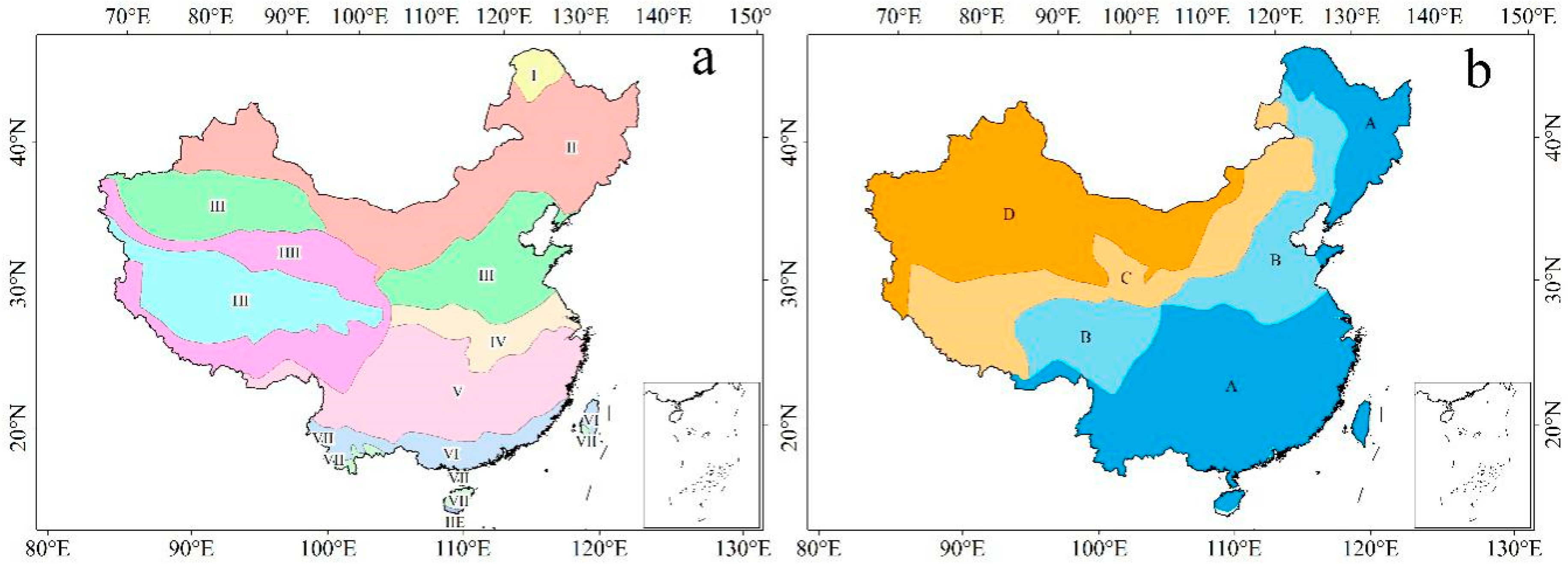
Figure 2 shows the respective distribution of temperature and humidity across China. The temperature and humidity data were obtained from the website: http://www.resdc.cn [41].
2.2. Direct Horizontal Irradiance Evaluation Model
2.2.1. Back Propagation Neural Network
BP is a supervised learning algorithm proposed by D.E. Rumelhart in 1986 [42]. The BP neural network is a three-layer structure that includes an input layer, an intermediate layer, and an output layer; the layers are interconnected but the nodes of each layer are not connected. In this study, for establishing the DHI calculation model, the basic structure of the BP neural network is 6-10-1. The air temperature (T), air pressure (PS), day number (D), relative humidity (RH), sunshine duration (SD), and altitude (A) are the input variables; the number of nodes in the hidden layer is 10; and one output variable of the model is the value of the daily DHI.
For the whole study period, a total of 70% of the datasets were modeled using the BP model, and the remaining datasets were used to evaluate it. The DHI values were calculated using the following equation:
where Mi is the estimated DHI, Z(.) is the hidden transfer function, wi(t) is the weight coefficient, xi(t) are the input variables and b is the neuronal bias.
2.2.2. General Regression Neural Network (GRNN)
A GRNN model is a type of radial basis function neural network (RBF). The classical generalized regressive neural network is a type of radial basis neural network [43]. It has a strong nonlinear mapping ability and flexibility, and the network structure has a high degree of fault tolerance and robustness. GRNN consists of a four-layer network, this is, the input layer, the mode layer, the summation layer and the output layer. Qin et al. [44] and Wang et at. [17] provide detailed information on the steps required for estimating DHI using the GRNN model using meteorological data.
2.2.3. Genetic Algorithm (Genetic)
Genetic is a metaheuristic proposed by Holland in 1969 [45], which consists of a class of evolutionary algorithms analog summarized by DeJong et al. [46] and Goldberg et al. [47]. Genetic is a type of self-organizing simulation of the natural process of biological evolution and the mechanisms needed to solve the problems of extreme values and is based on adaptive artificial intelligence technology. We used BP neural networks to determine the weights and thresholds of the optimization needed to improve the accuracy of the model for predicting DHI values. Based on the basic structure of BP neural network 6-10-1 above, therefore, when the genetic algorithm initializes the random population, the number of weights is 70 (6 × 10 + 10 × 1) and the number of thresholds is 11 (10 + 1). The coding length of Genetic for estimating the daily DHI is 81 (70 + 11). A detailed explanation of Genetic used to estimate DHI is given in Wang et al. [17].
2.2.4. M5 Model Tree (M5Tree)
M5Tree was based on a binary decision tree with linear regression functions at the terminal (leaf) nodes [48], which was first developed by Quinlan [49]. This model is based on the classification tree to create a relationship between the dependent and independent variables. Evaluating with M5Tree generally consists of three steps [50,51]: (1) divide the data into subsets to create a decision tree; (2) generate a model tree based on the decision tree; and (3) construct a linear regression model. The schematic diagram of M5Tree can be obtained in Wang et al [52]. The standard deviation reduction (SDR) can be expressed by the following formula:
where E is the set of examples of reaching the node, SD is the standard deviation.
2.2.5. Multivariate Adaptive Regression Splines (MARS)
MARS is a form of non-parametric regression technique [53]. The MARS consecutive relevant prediction model utilizes a set of independent variables or variable value predictors, and generally operates without assuming a functional relationship between the dependent and independent variables [54]. The general MARS model equation for estimating DHI values is expressed as follows:
where V is the estimated DHI values, which is a function of the input parameters (RH, T, PS, SD, A and day number); α is the intercept parameter; βm is the weight of the input parameters; and hm (X) is the basis function.
2.2.6. Yang’s Hybrid Model (YHM)
The physical parameterization scheme of Yang’s Hybrid model [55] takes into account the five solar radiation transmittance of the atmosphere during damping (aerosol extinction, ozone absorption, Rayleigh scattering, gas absorption and water vapor absorption). It can be expressed as follows:
where Hall (MJ m−2day−1) is the daily DHI for all-sky conditions and Hclr is the daily DHI for clear-sky conditions. τc is a cloud transmittance parameter to corrected the cloud effect on daily DHI, which is a function of the SD and the maximum possible sunshine durations (N) [35].
Hall = τc Hclr
2.3. Statistical Measures of Model Accuracy
We used regression analysis between the measured and estimated values of DHI to validate the accuracy of the DHI models. The mean absolute bias error (MAE), mean bias errors (MBE), root mean square error (RMSE), coefficient of determination (R2) and correlation coefficient (R) were used for the evaluation. They were calculated as follows:
Here, N represent the number of samples collected; and represent the estimated and observed DHI, respectively; represents the mean value of the estimated DHI; and represent the mean value of the observed DHI.
2.4. Data Quality Control
The DHI data from CMA used for model evaluation in this study covered the 57-year interval from 1960–2016. Three different classes (first class, second class and third class) of radiometer were installed for measuring solar radiation in China both before 1990 and subsequent to (Table 1). However, only first-class stations (16 stations) could measure DHI from 1960 to the present. It is reported that observed DHI data may have an inhomogeneity problem because of the sensitivity drift and instrument replacement [55]; therefore, daily DHI observations at these stations should be checked to ensure data quality. Detailed rules for assessing these data are given in Tang et al. [56]. After the quality control, the remaining data were used for model estimation and accuracy verification. In addition, quality control of all the other daily meteorological data was performed by CMA, and the detailed procedures are given at http://data.cma.gov.cn [57].
3. Results and Discussion
To ensure the accuracy and effectiveness of the experimental results, 10,752 samples (the compilations of the estimated results of BP, GRNN, Genetic, M5Tree, MARS and YHM at 16 CMA stations) were taken to verify the accuracy of the models during 1960–2016.
3.1. Validation of Estimated DHI
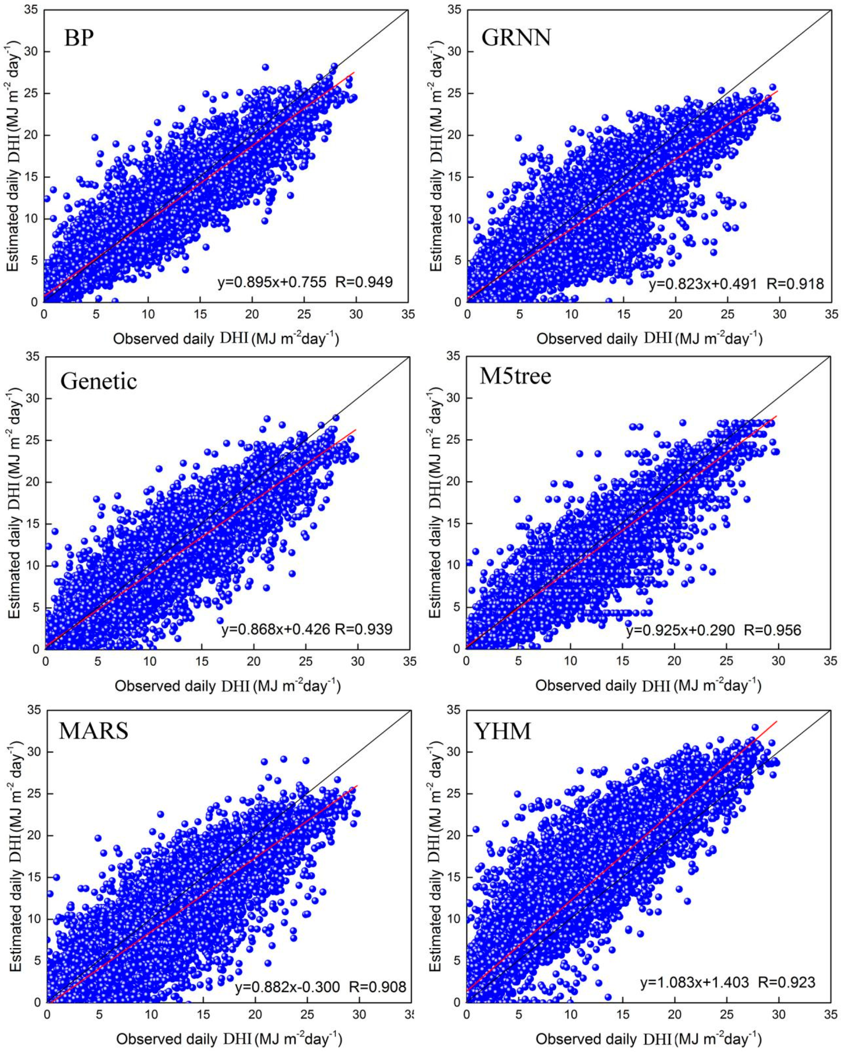
Correlation analysis was used to analyze the differences between the observed and estimated daily DHI for BP, GRNN, Genetic, M5Tree, MARS, and YHM at 16 CMA stations. The results are shown in Figure 3 and they indicate that the estimated values of DHI simulated by BP, GRNN, Genetic, M5Tree, MARS and YHM are all positively correlated with the DHI measurements; the correlation coefficients are 0.949, 0.918, 0.939, 0.956, 0.908 and 0.923, respectively. For the 16 CMA stations, M5Tree yielded slightly better forecasts (RMSE = 1.989, MAE = 1.923, R2 = 0.915) than BP (RMSE = 2.122, MAE = 1.440, R2 = 0.901), GRNN (RMSE = 2.784, MAE = 1.788, R2 = 0.843), Genetic (RMSE = 2.390, MAE = 1.618, R2 = 0.882) and MARS (RMSE = 3.090, MAE = 2.250, R2 = 0.825). YHM, which is based on the theoretical principles of atmospheric physical transmission processes, also showed a relatively high degree of accuracy (RMSE = 3.692, MAE = 2.463, R2 = 0.853); however, it performed the worst among the six models, because of the effects of cloud, aerosol extinction and water vapor.
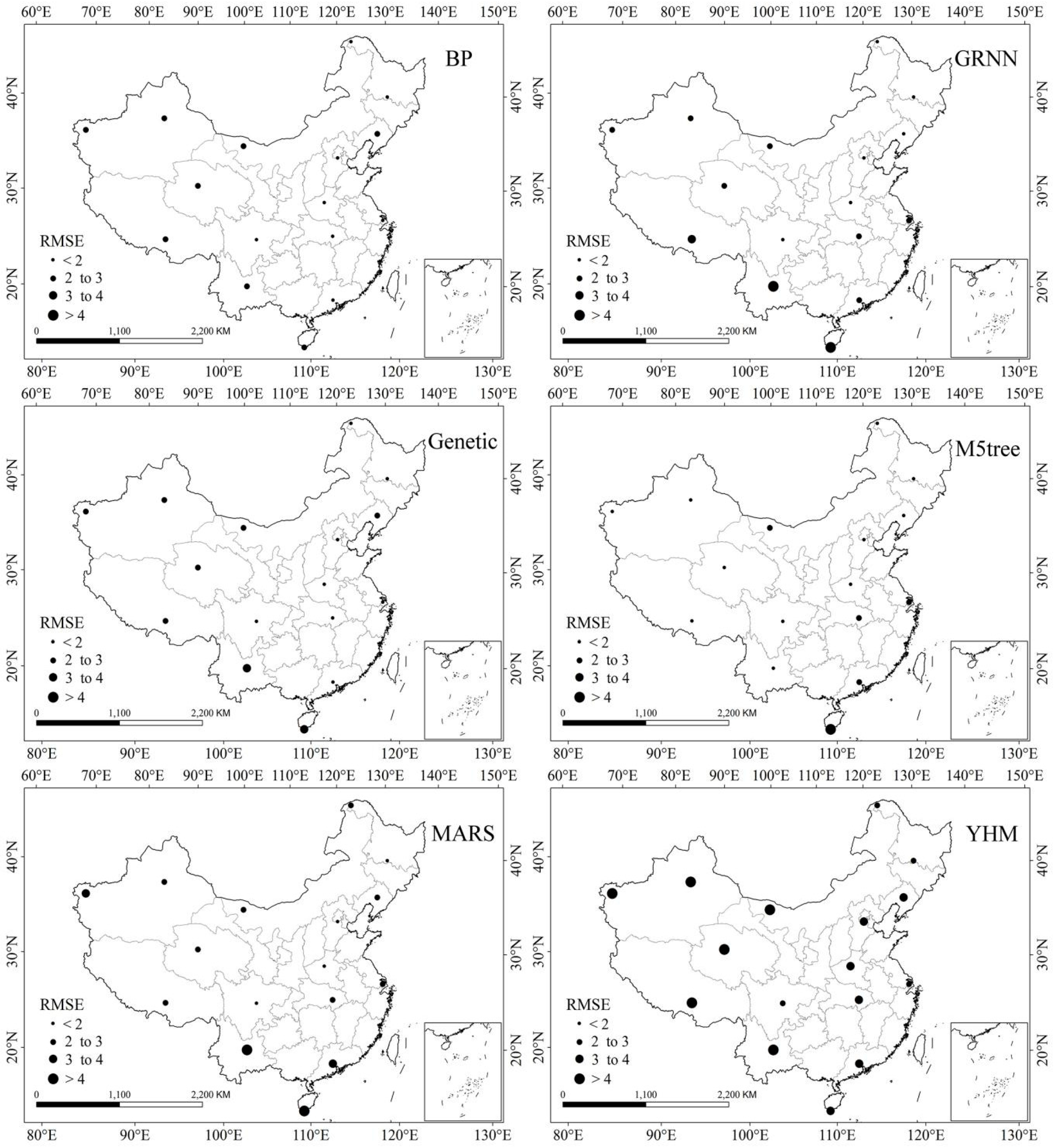
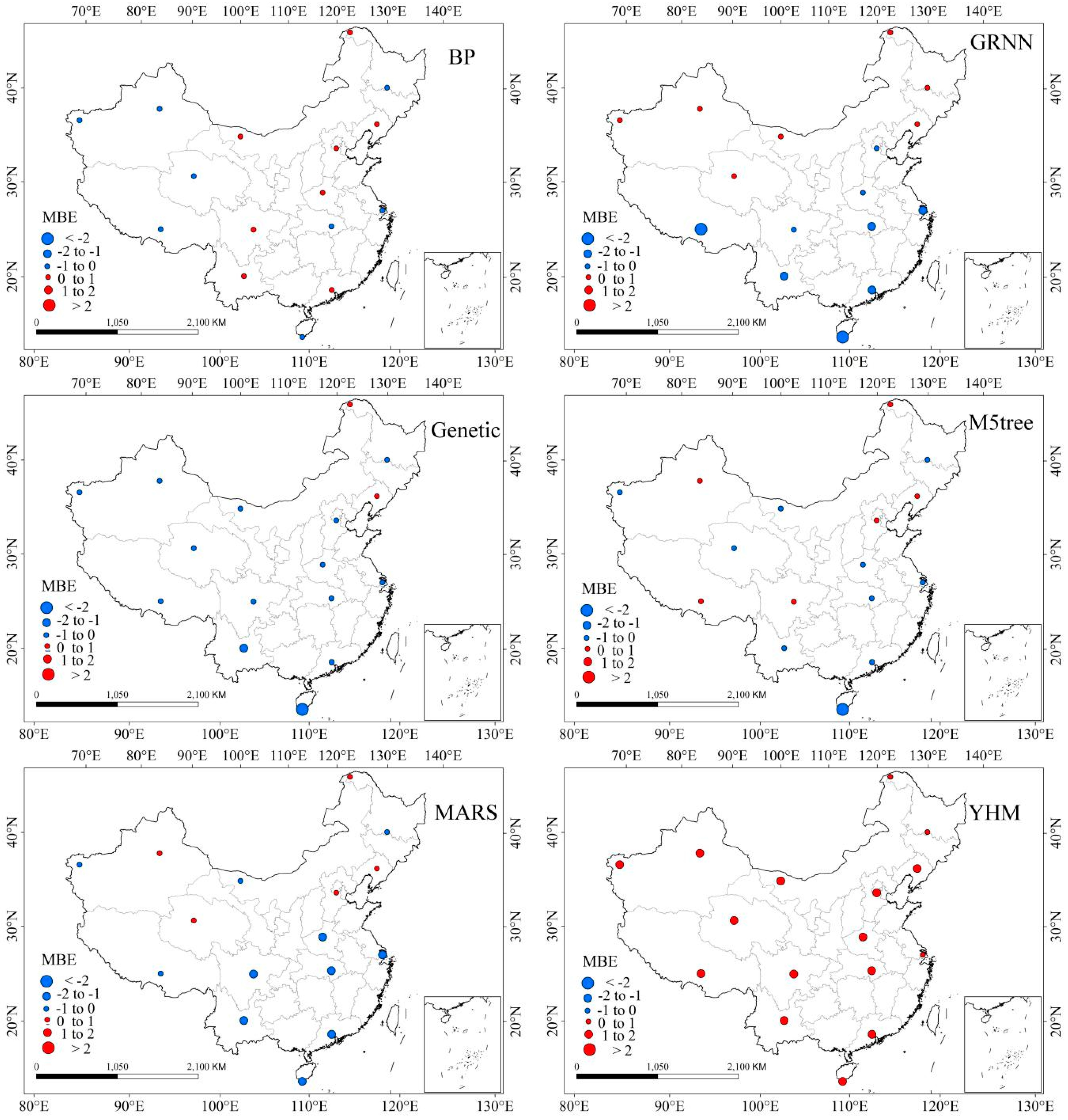
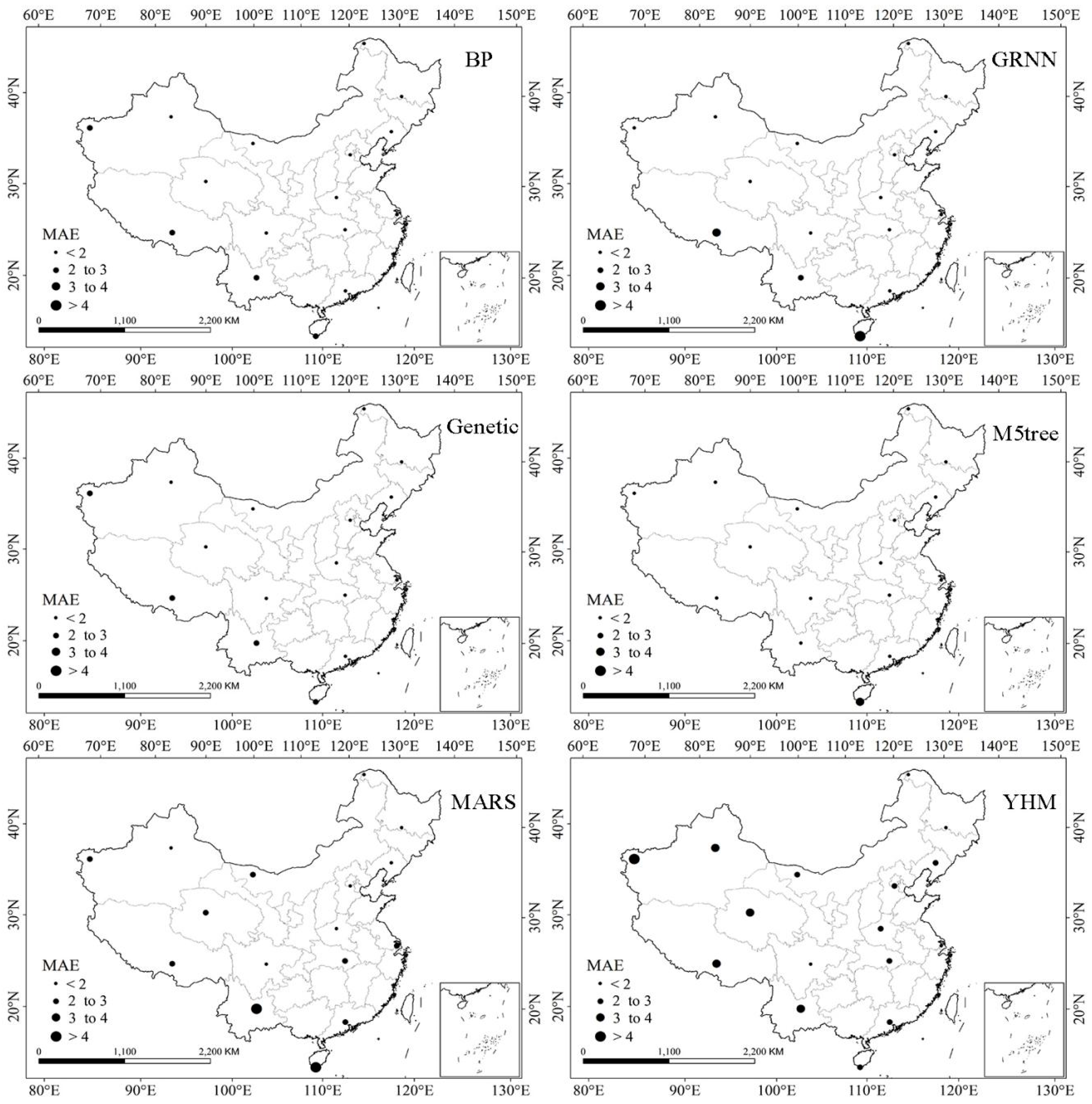
Figure 4, Figure 5 and Figure 6 illustrate spatial changes of the mean values of the statistical indicators (RMSE, MBE and MAE), representing the accuracy of the six different DHI models. It is evident that all model performances are better in the eastern regions than in the western regions of China. In addition, the M5Tree model is overwhelmingly superior to the other DHI models, because of its strong self-learning ability. The values of RMSE, MAE, and R2 for M5Tree are 1.839, 1.194 MJ m−2day−1 and 0.899, respectively. The SHY station in Hainan province has the largest MAE (3.028 MJ m−2day−1), MBE (−2.371 MJ m−2day−1), and RMSE (4.258 MJ m−2day−1) for M5Tree. The lowest MAE and RMSE are 0.380 and 0.781 MJ m−2day−1, respectively, and are for WJ station in the southern Sichuan. YHM was not as accurate as the other DHI models, because of its vulnerability to cloud and terrain effects; for this model, RMSE, MAE and R2 are 3.554, 2.468 MJ m−2day−1 and 0.837, respectively. The highest RMSE and MAE (5.830 and 4.589 MJ m−2day−1, respectively) are for YHM of KAS station in northwestern Xinjiang, possibly because of the high atmospheric dust loading. The lowest RMSE and MAE (2.066 and 1.302 MJ m−2day−1, respectively) are for MH station in northeastern Heilongjiang, because of the low radiative damping processes in the region.
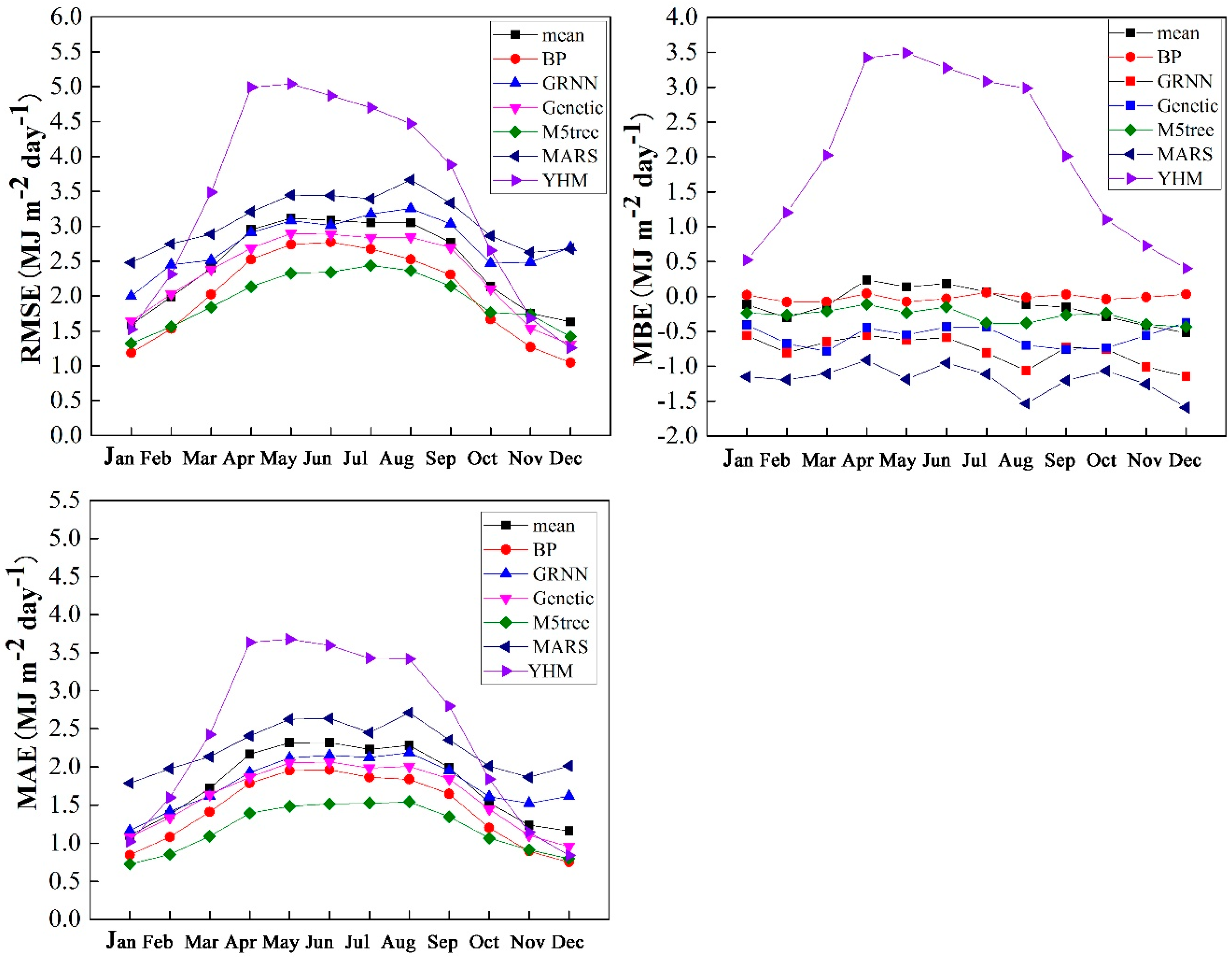
Figure 7 shows the monthly changes of RMSE, MBE and MAE for BP, GRNN, Genetic, M5Tree, MARS and YHM. The results show that the model measurements are better in winter than in summer, because of the relatively strong radiative damping processes due to frequent cloud occurrence and wet weather in summer. The mean MAE and RMSE in May are 2.318 and 3.255 MJ m−2day−1, respectively, which are the highest values. The minimum mean values of MAE and RMSE are 1.105 and 1.690 MJ m−2day−1, respectively, and are observed in January. In addition, the RMSE and MAE values from winter to summer show an increasing trend. The lowest mean MAE and RMSE are 1.215 and 1.736 MJ m−2day−1, respectively, and are observed in winter; while the highest mean MAE and RMSE are 2.277 and 3.061 MJ m−2day−1, respectively, and are observed in summer. M5tree performed better than BP, GRNN, Genetic, MARS and YHM in most months of the year. The largest RMSE for M5Tree is 2.438 MJ m−2day−1 in July, while the smallest RMSE is 1.323 MJ m−2day−1 in January; the largest MAE for M5Tree is 1.526 MJ m−2day−1 in July, and the lowest MAE is 0.724 MJ m−2day−1 in January. Although the RMSE varies for YHM and BP, GRNN, Genetic, M5tree and MARS, they all show a similar pattern of significant seasonal changes because of strong radiative damping processes in summer. The highest MAE and RMSE for YHM are 3.676 and 5.041 MJ m−2day−1, respectively, and are observed in May; and the lowest lest MAE and RMSE are 0.842 and 1.258 MJ m−2day−1, respectively, and are observed in December.
In summary, M5Tree was superior to the other DHI models in stations with smaller seasonal variations, which suggests that this model can be used to reconstruct the historical datasets of DHI at CMA stations across mainland China, with a high degree of accuracy and robustness.
3.2. Analysis of Spatial-Temporal Variations of DHI Values across China
Daily meteorological data from 839 CMA stations across China were used as input data using the M5Tree model to simulate the daily average DHI values for 1960–2016. The monthly and annual mean DHI values were calculated and software tools in ArcGIS were used to illustrate the temporal trend of annual average DHI.
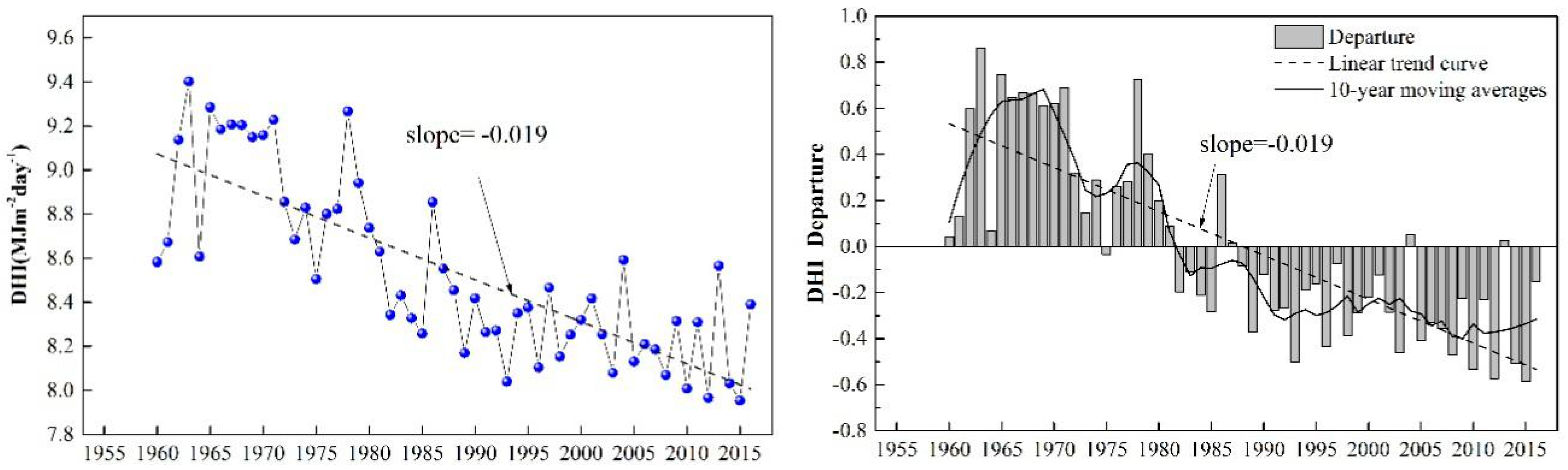
Figure 8 illustrates the temporal trends of the annual mean values of DHI during 1960–2016 across mainland China. The results indicate that the highest value occurs in 1963 (9.402 MJm−2day−1) and the lowest value in 2015 (7.954 MJm−2day−1). The DHI values decrease at the rate of −0.190 MJm−2day−1 per decade during 1960–2016. Especially after 1980, the annual mean DHI values decreased gradually, because of the enhancement of the aerosol radiative forcing effect with the population growth and rapid development of the economy [44]. In 1990–2007, the annual mean DHI decreased slowly, at the rate of 0.027 MJm−2 day−1 per decade, and the annual mean DHI increased at the rate of 0.084 MJm−2day−1 per decade during 2008–2016; this is because the aerosol radiative forcing effect was decreasing as a consequence of the further implementation of environmental protection policies [44]. The trend of the DHI in the research matched the previous finding in Athens [60], the Mediterranean Basin [61], the Indian monsoon region [62], China and Japan [63], all of which reveal the “global dimming/brightening“ effect. The difference of the result illustrates that the affecting factors on the trends change of DHI change with climate, topography, humidity, cloud, and aerosol effects.
Figure 9 indicates the spatial pattern of the annual average DHI values over mainland China. The values increased gradually from southeast China to northwest China, from 3.481–17.495 MJ m−2day−1 with an average of ~9.836 MJm−2day−1. The pattern of annual mean DHI is spatially heterogeneous across the mainland; for example, the maximum DHI value (17.195 MJ m−2day−1) occurs on the Tibetan Plateau. Northwest China and the Mongolian Plateau also exhibit high values (12.542 MJ m−2day−1), whereas the lowest values (from 3.481 MJ m−2day−1 to 7.460 MJ m−2day−1) occur in the southeastern part of the Yunnan–Guizhou Plateau, the Sichuan Basin and most of the southern Yangtze River Basin.
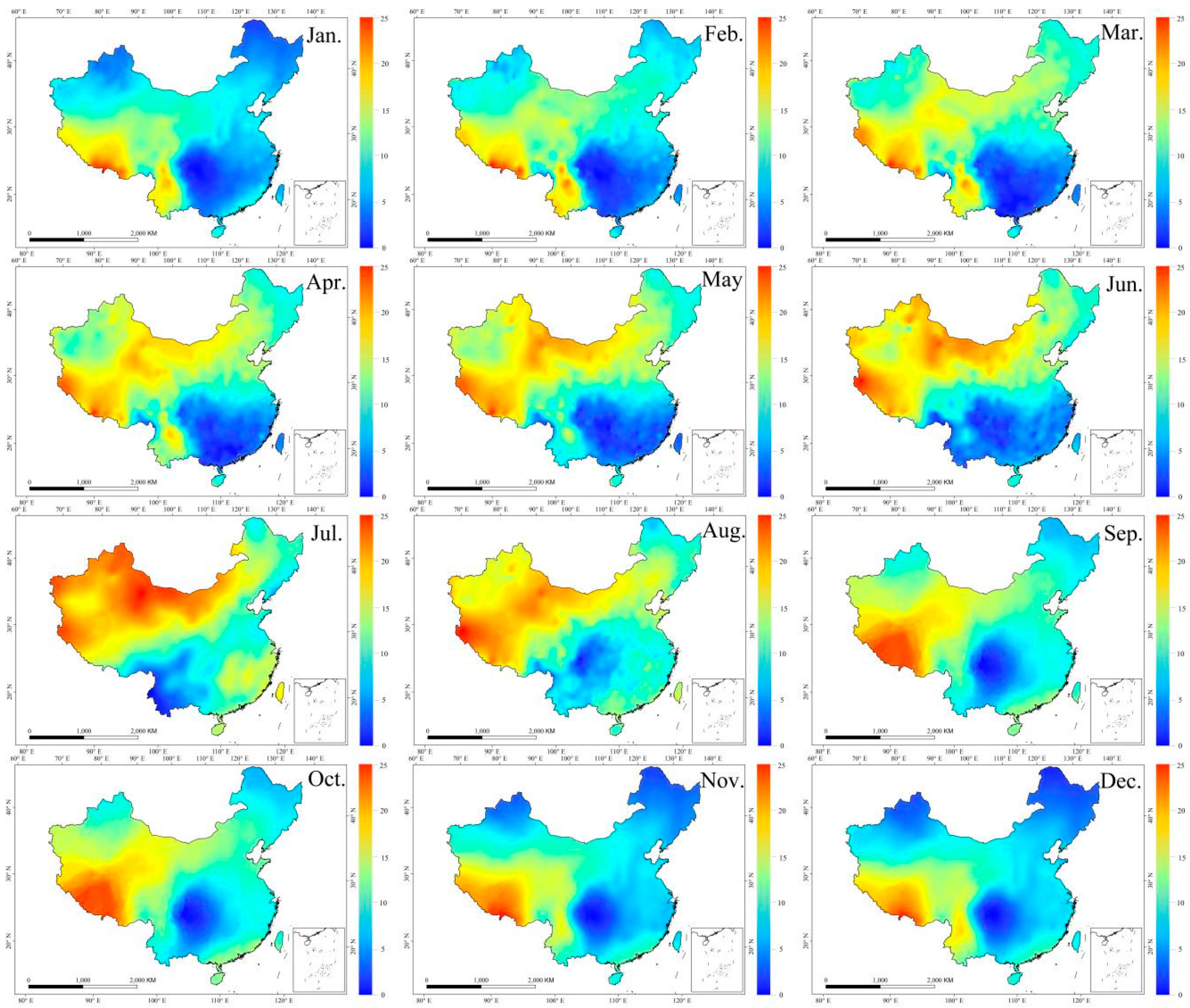
The spatial pattern of monthly DHI in China is shown in Figure 10. Here, spring is March–May, summer is June–August, autumn is September–November, and winter is December–February. The sunshine duration in summer is longer and the daily average solar elevation angle higher than in other seasons, because China is in the middle and low latitudes of the Northern Hemisphere. Therefore, the DHI value in summer (13.185 MJ m−2day−1) over mainland China is significantly higher than in spring (11.046 MJ m−2day−1), autumn (8.609 MJ m−2day−1) and winter (7.218 MJ m−2day−1).
The monthly and annual DHI values of the Qinghai–Tibetan Plateau are the highest because of the lowest attenuation of the solar rays due to the high attitude. For the Qinghai–Tibetan Plateau, the annual mean DHI during 1960-2016 is 13.43 MJ m−2day−1, and the values range from 8.522 MJ m−2day−1 (January) to 17.946 MJ m−2day−1 (May). The annual DHI value of the Mongolian Plateau is 11.49 MJ m−2day−1, which is because this arid region has less precipitation and a higher frequency of sunny days than elsewhere, and thus the attenuation of solar radiation by the thin atmosphere is weak [35,64].
The Sichuan Basin lies within the warm and humid climate zone, and there is a high incidence of cloud and fog throughout the year. In addition to the basin terrain, aerosol particles and clouds result in the substantial attenuation of atmospheric radiation; therefore, the Sichuan Basin has low values of direct radiation in China, and its annual mean DHI is 6.478 MJ m−2day−1. The monthly mean DHI values for the Sichuan Basin from January to December are 5.45, 7.09, 7.608, 7.256, 10.24, 9.976, 7.35, 5.91, 4.754, 3.952, 3.697 and 4.35 MJ m−2day−1, respectively. The middle and lower reaches of the Yangtze River (MLYR) and the Chiang-nan Hilly Region (CHR) have consistently low values because of the influence of the monsoon in spring and summer, because solar radiation receipt is reduced during the rainy season. The ranges of the monthly mean DHI values in Hanzhong Basin, the MLYR, and the CHR are 5.08–9.62 MJ m−2day−1, 5.31–9.34 MJ m−2day−1, and 3.47–13.65 MJ m−2day−1, respectively.
Because of its low latitude and short sunshine duration, northeast China is characterized by low values in winter; for example, the annual DHI value of the Greater Khingan Range is 7.282 MJ m−2day−1. In the desert regions of northwestern China, although aerosols in the desert can weaken the effects of solar radiation, because of the perennial arid climate conditions in the region, the solar radiation attenuation effect is weak, so the annual average solar radiation on the surface is higher.
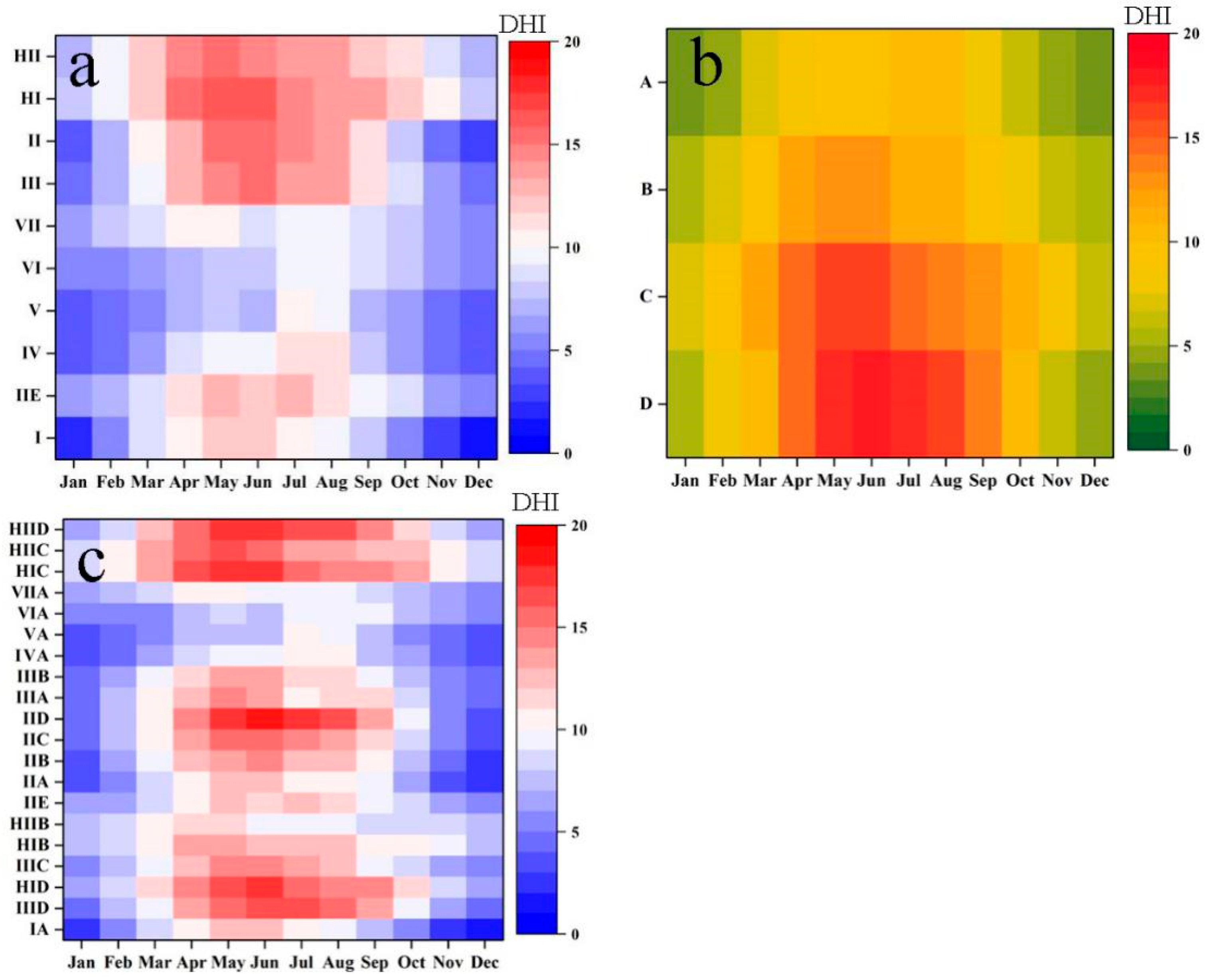
Figure 11 shows the monthly average DHI values in different climatic zones. Because cloud cover is the dominant factor affecting surface solar radiation [35], the DHI values are generally higher in semi-arid and arid zones than in humid zones, which have a more frequent cloud occurrence. The ranges of DHI for HIC, HIIC, HID and IID are 8.52–17.94, 8.42–16.54, 6.36–16.54, and 3.90 –18.08 MJ m−2day−1, respectively; and the ranges of VIA, IVA, IIE, VIIA, IIA, IA and IIIA are 3.697–10.243, 5.069–9.885, 3.815–10.965, 5.505–12.663, 5.72–10.59, 2.253–12.42, 1.519–12.419 and 4.004–14.503 MJm−2day−1, respectively. Notably, the DHI values during May–August are 14.286–18.955 MJ m−2day−1 in the arid zones, and 8.24–10.06 MJ m−2day−1 in the humid zones. Thus, DHI is higher in the semi-arid and arid zones than in the humid and semi-humid zones, especially during May to August, because of the perennial rainy weather in the latter and the resulting attenuation effect of clouds and water vapor. For example, the DHI values for HIC, HIIC, HID, and IID in summer are 14.606–17.361 MJ m−2day−1, 13.264–15.581 MJ m−2day−1, 14.849–17.045 MJ m−2day−1 and 16.262–18.079 MJm−2day−1, respectively; and the values for VA, VIA, IVA, IIE, VIIA, IIA, IA, IIIA are 7.61–10.24, 7.88–9.86, 9.84–10.97, 11.19–12.66, 9.03–10.59, 10.24–12.42, 9.30–12.42, and 10.27–14.50 MJ m−2day−1,respectively.
4. Conclusions
Solar radiation stations are extremely sparsely distributed across China, and, therefore, they are unable to meet the requirements for the optimum location of solar power thermal plants, especially for planning CSP systems. Therefore, we conducted a systematic study of six different models (a physically based model and five machine learning methods) to estimate daily DHI. The accuracies of the DHI estimates using the six different models are comparable to those at the 16 CMA DHI stations; however, the M5Tree method for daily DHI estimation exhibits the best performance, with RMSE and MAE being about 1.989 and 1.923 MJ m−2day−1, respectively, for different climatic conditions across China.
We extended the method to compile a dataset from 839 CMA meteorological stations using the M5Tree model and then investigated the spatiotemporal distribution of DHI across China. There was a significant decreasing trend for DHI, at a rate of −0.19 MJm−2 per decade, during 1960–2016. The annual mean DHI was generally higher in the Qinghai−Tibetan Plateau (13.43 MJ m−2day−1) and the Mongolian Plateau, and lower in the Yunnan−Guizhou Plateau, the Sichuan Basin (6.478 MJ m−2day−1) and most of the southern Yangtze River Basin.
Our various analyzed DHI datasets from 1960 to 2016 for China potentially have applications in fields such as global and regional climatology, agricultural production, and especially in the application of CSP thermal systems throughout China. Our study also provides a refined methodology for estimating DHI. Finally, we suggest that these models should be further tested and verified in other climatic zones and terrain types worldwide. This study is the first assessment of various DHI models in different ecosystems, and derives a long-term high-density dataset of daily DHI in China, which contributes to many aspects, such as terrestrial ecosystem processes, solar energy technologies, and especially CSP thermal systems. Meanwhile, the effects of water vapor, aerosols, and cloud, as well as on the temporal variations of DHI will be quantitatively analyzed in future work. Although we have done the variable selection and parameter tuning in preparatory work, the parameter selection and tuning could be further improved in future work. Especially, the mean impact value (MIV) method proposed by Dombi et al. [65] will be used for variable selection and the Bayesian optimization method will be used to tune the hyper parameters for AI models.
Author Contributions
Conceptualization, A.L. and W.Q.; methodology, F.C. and W.Q. and J.N.; data curation, F.C.; writing—original draft preparation, Z.Z. and F.C.; writing—review and editing, F.C. and Z.Y.
Funding
This research was funded by the National Natural Science Foundation of China (grant number.41771438 and grant number.41671405) and the Henan Province Philosophy and Social Science planning project (grant number.2016JJ046).
Acknowledgments
The CMA station data were obtained from the National Meteorological Information Center, which was highly appreciated by the authors.
Conflicts of Interest
The authors declare no conflict of interest.
References
- Wang, L.; Gong, W.; Hu, B.; Lin, A.; Li, H.; Zou, L. Modeling and analysis of the spatiotemporal variations of photosynthetically active radiation in China during 1961–2012. Renew. Sustain. Energy Rev. 2015, 49, 1019–1032. [Google Scholar] [CrossRef]
- Wang, B.; Shi, G. Long-term trends of atmospheric absorbing and scattering optical depths over China region estimated from the routine observation data of surface solar irradiances. J. Geophys. Res. Atmos. 2010, 115. [Google Scholar] [CrossRef] [Green Version]
- Liu, Z.; Wu, D.; Yu, H.; Ma, W.; Jin, G. Field measurement and numerical simulation of combined solar heating operation modes for domestic buildings based on the Qinghai-Tibetan plateau case. Energy Build. 2018, 167, 312–321. [Google Scholar] [CrossRef]
- National Energy Administration: Statistics of photovoltaic power generation in 2016. Available online: http://www.nea.gov.cn/2017-02/04/c_136030860.htm (accessed on 26 September 2018).
- Mellit, A.; Eleuch, H.; Benghanem, M.; Elaoun, C.; Pavan, A.M. An adaptive model for predicting of global, direct and diffuse hourly solar irradiance. Energy Convers. Manag. 2010, 51, 771–782. [Google Scholar] [CrossRef]
- Sun, H.; Qiang, Z.; Wang, Y.; Yao, Q.; Su, J. China’s solar photovoltaic industry development: The status quo, problems and approaches. Appl. Energy 2014, 118, 221–230. [Google Scholar] [CrossRef]
- Qin, J.; Tang, W.; Yang, K.; Lu, N.; Niu, X.; Liang, S. An efficient physically based parameterization to derive surface solar irradiance based on satellite atmospheric products. J. Geophys. Res. Atmos. 2015, 120, 4975–4988. [Google Scholar] [CrossRef] [Green Version]
- Tang, W.; Qin, J.; Yang, K.; Liu, S.; Lu, N.; Niu, X. Retrieving high-resolution surface solar radiation with cloud parameters derived by combining MODIS and MTSAT data. Atmos. Chem. Phys. 2015, 16, 2543–2557. [Google Scholar] [CrossRef]
- Sanchez-Lorenzo, A.; Enriquez-Alonso, A.; Wild, M.; Trentmann, J.; Vicente-Serrano, S.M.; Sanchez-Romero, A.; Posselt, R.; Hakuba, M.Z. Trends in downward surface solar radiation from satellites and ground observations over Europe during 1983–2010. Remote Sens. Environ. 2017, 189, 108–117. [Google Scholar] [CrossRef]
- Pinker, R.T.; Laszlo, I. Modeling Surface Solar Irradiance for Satellite Applications on a Global Scale. J. Appl. Meteorol. 1992, 31, 194–211. [Google Scholar] [CrossRef] [Green Version]
- Rossow, W.B. Advances in understanding clouds from ISCCP. Bull. Am. Meteorol. Soc. 1999, 80, 2261–2287. [Google Scholar] [CrossRef]
- Zhang, Y.C.; Rossow, W.B.; Lacis, A.A. Calculation of surface and top of atmosphere radiative fluxes from physical quantities based on ISCCP data sets: 1. Method and sensitivity to input data uncertainties. J. Geophys. Res. Atmos. 1995, 100, 1149–1165. [Google Scholar] [CrossRef]
- Kalnay, E.; Kanamitsu, M.; Kistler, R.; Collins, W.; Deaven, D.; Gandin, L.; Iredell, M.; Saha, S.; White, G.; Woollen, J. The NCEP/NCAR 40-Year Reanalysis Project. Bull. Am. Meteorol. Soc. 1996, 77, 437–472. [Google Scholar] [CrossRef]
- Kistler, R.; Collins, W.; Saha, S.; White, G.; Woollen, J.; Kalnay, E.; Chelliah, M.; Ebisuzaki, W.; Kanamitsu, M.; Kousky, V. The NCEP–NCAR 50–Year Reanalysis: Monthly Means CD–ROM and Documentation. Bull. Am. Meteorol. Soc. 2001, 82, 247–268. [Google Scholar] [CrossRef]
- Kobayashi, S.; Ota, Y.; Harada, Y.; Ebita, A.; Moriya, M.; Onoda, H.; Onogi, K.; Kamahori, H.; Kobayashi, C.; Endo, H. The JRA-55 Reanalysis: General Specifications and Basic Characteristics. J. Meteorol. Soc. Jpn. Ser. II 2015, 93, 5–48. [Google Scholar] [CrossRef] [Green Version]
- Zhang, X.; Liang, S.; Wang, G.; Yao, Y.; Jiang, B.; Cheng, J. Evaluation of the Reanalysis Surface Incident Shortwave Radiation Products from NCEP, ECMWF, GSFC, and JMA using Satellite and Surface Observations. Remote Sens. 2016, 8, 225. [Google Scholar] [CrossRef]
- Wang, L.; Kisi, O.; Zounemat-Kermani, M.; Salazar, G.A.; Zhu, Z.; Gong, W. Solar radiation prediction using different techniques: Model evaluation and comparison. Renew. Sustain. Energy Rev. 2016, 61, 384–397. [Google Scholar] [CrossRef]
- Wang, L.; Kisi, O.; Zounemat Kermani, M.; Zhu, Z.; Gong, W.; Niu, Z.; Liu, H.; Liu, Z. Prediction of solar radiation in China using different adaptive neuro-fuzzy methods and M5 model tree. Int. J. Clim. 2016, 37, 1141–1155. [Google Scholar] [CrossRef]
- Qin, W.; Wang, L.; Lin, A.; Zhang, M.; Xia, X.; Hu, B.; Niu, Z. Comparison of deterministic and data-driven models for solar radiation estimation in China. Renew. Sustain. Energy Rev. 2018, 81, 579–594. [Google Scholar] [CrossRef]
- Keshtegar, B.; Mert, C.; Kisi, O. Comparison of four heuristic regression techniques in solar radiation modeling: Kriging method vs RSM, MARS and M5 model tree. Renew. Sustain. Energy Rev. 2018, 81, 330–341. [Google Scholar] [CrossRef]
- Liu, Z.; Li, H.; Liu, K.; Yu, H.; Cheng, K. Design of high-performance water-in-glass evacuated tube solar water heaters by a high-throughput screening based on machine learning: A combined modeling and experimental study. Sol. Energy 2017, 142, 61–67. [Google Scholar] [CrossRef]
- Deo, R.C.; Şahin, M. Forecasting long-term global solar radiation with an ANN algorithm coupled with satellite-derived (MODIS) land surface temperature (LST) for regional locations in Queensland. Renew. Sustain. Energy Rev. 2017, 72, 828–848. [Google Scholar] [CrossRef]
- Ertekin, C.; Evrendelik, F. Spatio-temporal modeling of global solar radiation dynamics as a function of sunshine duration for Turkey. Agric. For. Meteorol. 2007, 145, 36–47. [Google Scholar] [CrossRef]
- Meza, F.; Varas, E. Estimation of mean monthly solar global radiation as a function of temperature. Agric. For. Meteorol. 2000, 100, 231–241. [Google Scholar] [CrossRef]
- Ehnberg, J.S.G.; Bollen, M.H.J. Simulation of global solar radiation based on cloud observations. Sol. Energy 2005, 78, 157–162. [Google Scholar] [CrossRef]
- Kambezidis, H.D. Current Trends in Solar Radiation Modeling: The Paradigm of MRM. J. Fundam. Renew. Energy Appl. 2016, 6, e106. [Google Scholar] [CrossRef]
- Kambezidis, H.D.; Psiloglou, B.E.; Karagiannis, D.; Dumka, U.C.; Kaskaoutis, D.G. Recent improvements of the Meteorological Radiation Model for solar irradiance estimates under all-sky conditions. Renew. Energy 2016, 93, 142–158. [Google Scholar] [CrossRef]
- Kambezidis, H.D.; Psiloglou, B.E.; Karagiannis, D.; Dumka, U.C.; Kaskaoutis, D.G. Meteorological Radiation Model (MRM v6.1): Improvements in diffuse radiation estimates and a new approach for implementation of cloud products. Renew. Sustain. Energy Rev. 2017, 74, 616–637. [Google Scholar] [CrossRef]
- Kambezidis, H.D. Solar Radiation Modelling: The Latest Version and Capabilities of MRM. J. Fundam. Renew. Energy Appl. 2017, 7. [Google Scholar] [CrossRef]
- Yao, W.; Zhang, C.; Wang, X.; Zhang, Z.; Li, X.; Di, H. A new correlation between global solar radiation and the quality of sunshine duration in China. Energy Convers. Manag. 2018, 164, 579–587. [Google Scholar] [CrossRef]
- Hassan, G.E.; Youssef, M.E.; Mohamed, Z.E.; Ali, M.A.; Hanafy, A.A. New Temperature-based Models for Predicting Global Solar Radiation. Appl. Energy 2016, 179, 437–450. [Google Scholar] [CrossRef]
- Yang, K.; Koike, T. A general model to estimate hourly and daily solar radiation for hydrological studies. Water Resour. Res. 2005, 41, W10403. [Google Scholar] [CrossRef]
- Yang, K.; Huang, G.W.; Tamai, N. A hybrid model for estimating global solar radiation. Sol. Energy 2001, 70, 13–22. [Google Scholar] [CrossRef]
- Çelik, Ö.; Teke, A.; Yıldırım, H.B. The optimized artificial neural network model with Levenberg–Marquardt algorithm for global solar radiation estimation in Eastern Mediterranean Region of Turkey. J. Clean Prod. 2016, 116, 1–12. [Google Scholar] [CrossRef]
- Tang, W.; Yang, K.; Qin, J.; Min, M.; Niu, X. First Effort for Constructing a Direct Solar Radiation Data Set in China for Solar Energy Applications. J. Geophys. Res. Atmos. 2018, 123, 1724–1734. [Google Scholar] [CrossRef]
- Bertrand, C.; Vanderveken, G.; Journée, M. Evaluation of decomposition models of various complexity to estimate the direct solar irradiance over Belgium. Renew. Energy 2015, 74, 618–626. [Google Scholar] [CrossRef]
- Arias Rosales, A.; Mejía Gutiérrez, R. Modelling and simulation of direct solar radiation for cost-effectiveness analysis of V-Trough photovoltaic devices. Int. J. Interact. Des. Manuf. (IJIDeM) 2016, 10, 257–273. [Google Scholar] [CrossRef]
- Gueymard, C.A. Direct solar transmittance and irradiance predictions with broadband models. Part I: Detailed theoretical performance assessment. Sol. Energy 2003, 74, 355–379. [Google Scholar] [CrossRef]
- Gueymard, C.A. Direct solar transmittance and irradiance predictions with broadband models. Part II: Validation with high-quality measurements. Sol. Energy 2003, 74, 381–395. [Google Scholar] [CrossRef]
- Chen, L.; He, L.; Chen, Q.; Zhu, H.; Wen, Z.; Wu, S. Study of monthly mean daily diffuse and direct beam radiation estimation with MODIS atmospheric product. Renew. Energy 2019, 132, 221–232. [Google Scholar] [CrossRef]
- Resource and Environment Data Cloud Platform (China). Available online: http://www.resdc.cn (accessed on 26 September 2018).
- Rumelhart, E.D.; Hinton, E.G.; Williams, J.R. Learning representations by back-propagating errors. Nature 1986, 323, 399–421. [Google Scholar] [CrossRef]
- Specht, D.F. A general regression neural network. IEEE Trans. Neural Netw. 1991, 2, 568–576. [Google Scholar] [CrossRef] [PubMed]
- Qin, W.; Wang, L.; Lin, A.; Zhang, M.; Bilal, M. Improving the Estimation of Daily Aerosol Optical Depth and Aerosol Radiative Effect Using an Optimized Artificial Neural Network. Remote Sens. 2018, 10, 1022. [Google Scholar] [CrossRef]
- Holland, J.H. Genetic Algorithms and Adaptation; Springer: Boston, MA, USA, 1984. [Google Scholar]
- Dejong, K. Learning with Genetic Algorithms: An Overview; Kluwer Academic Publishers: Dordrecht, The Netherlands, 1988. [Google Scholar]
- Goldberg, E.D.; Smith, E.R. Nonstationary function optimization using genetic algorithm with dominance and diploidy. In Proceedings of the ICGA 1987, Cambridge, MA, USA, 28–31 July 1987. [Google Scholar]
- Witten, I.H.; Frank, E. Data Mining: Practical Machine Learning Tools with Java Implementations. ACM Sigmod Rec. 1999, 31, 76–77. [Google Scholar] [CrossRef]
- Quinlan, J.R. Learning with Continuous Classes. In Proceedings of the 5th Australian Joint Conference on Artificial Intelligence, Hobart, Australia, 16–18 November 1992; pp. 343–348. [Google Scholar]
- Rahimikhoob, A.; Asadi, M.; Mashal, M. A Comparison Between Conventional and M5 Model Tree Methods for Converting Pan Evaporation to Reference Evapotranspiration for Semi-Arid Region. Water Resour. Manag. 2013, 27, 4815–4826. [Google Scholar] [CrossRef]
- Mirabbasi, R.; Kisi, O.; Sanikhani, H.; Gajbhiye Meshram, S. Monthly long-term rainfall estimation in Central India using M5Tree, MARS, LSSVR, ANN and GEP models. Neural Comput. Appl. 2018, 1–20. [Google Scholar] [CrossRef]
- Wang, L.; Kisi, O.; Hu, B.; Bilal, M.; Zounemat-Kermani, M.; Li, H. Evaporation modelling using different machine learning techniques. Int. J. Clim. 2017, 37, 1076–1092. [Google Scholar] [CrossRef]
- Friedman, J.H. Multivariate Adaptive Regression Splines. Ann. Stat. 1991, 19, 1–67. [Google Scholar] [CrossRef] [Green Version]
- Samui, P.; Karup, P. Multivariate adaptive regression spline and least square support vector machine for prediction of undrained shear strength of clay. Int. J. Appl. Metaheuristic Comput. 2012, 3, 33–42. [Google Scholar] [CrossRef]
- Yang, K.; Koike, T.; Ye, B. Improving estimation of hourly, daily, and monthly solar radiation by importing global data sets. Agric. For. Meteorol. 2006, 137, 43–55. [Google Scholar] [CrossRef]
- Tang, W.J.; Yang, K.; Qin, J.; Cheng, C.C.K.; He, J. Solar radiation trend across China in recent decades: A revisit with quality-controlled data. Atmos. Chem. Phys. 2011, 10, 393–406. [Google Scholar] [CrossRef]
- National Meteorological Information Center (China). Available online: http://data.cma.cn (accessed on 28 December 2018).
- Zhang, W. Technical report on telemetering radiometer. Meteorol. Mon. 1988, 7, 3. [Google Scholar]
- Zhang, W. Introduction to telemery radiation instruments and methods of observation. Meteorol. Mon. 1990, 26, 17–19. [Google Scholar]
- Kambezidis, H.D. The solar radiation climate of Athens: Variations and tendencies in the period 1992–2017, the brightening era. Sol. Energy 2018, 173, 328–347. [Google Scholar] [CrossRef]
- Kambezidis, H.D.; Kaskaoutis, D.G.; Kalliampakos, G.K.; Rashki, A.; Wild, M. The solar dimming/brightening effect over the Mediterranean Basin in the period 1979–2012. J. Atmos. Sol. Terr. Phys. 2016, 150–151, 31–46. [Google Scholar] [CrossRef]
- Kumari, B.P.; Goswami, B.N. Seminal role of clouds on solar dimming over the Indian monsoon region. Geophys. Res Lett. 2010, 37, 460–472. [Google Scholar]
- Norris, J.R.; Wild, M. Trends in aerosol radiative effects over China and Japan inferred from observed cloud cover, solar “dimming,” and solar “brightening”. J. Geophys. Res. 2009, 114. [Google Scholar] [CrossRef] [Green Version]
- Patton, R.W. The investigation of the nature and extent of attenuation of 3.2-cm radiation by subtropical precipitation. Master’s Thesis, Texas A & M University, College Station, TX, USA, 1965. [Google Scholar]
- József, D. Bayes theorem, uninorms and aggregating expert opinions. In Aggregation Functions in Theory and in Practise; Springer: Berlin, Germany, 2013. [Google Scholar]
Figure 1.
Distribution of the 16 direct horizontal irradiance (DHI) stations and 839 China Meteorological Administration (CMA) stations across China used as data sources (GKR for the Greater Khingan Range; IMP for the Inner Mongolia High Plain; TP for the Tibet Plateau; SB for the Sichuan Basin; YRB for the Yangtze River Basin).

Figure 2.
Climatic and humidity zones of China. (a) Temperate zones (I. cold temperate, II. mid-temperate, III. warm temperate, IV. northern subtropical, V. mid-subtropical, VI. southern subtropical, VII. tropical margin zone, HI. sub-frigid plateau zone, HII. plateau temperature zone, IIE. mid-tropical zone with humid weather. (b) Humidity zones (A. humid region, B. semi-humid region, C. semi-arid region, D. arid region).

Figure 3.
Results of correlation analysis of observed and estimated daily DHI at 16 CMA stations. Back propagation neural networks (BP); general regression neural networks (GRNN); genetic algorithm (Genetic); M5 model tree (M5Tree); multivariate adaptive regression splines (MARS); 343 Yang’s hybrid model (YHM).

Figure 4.
Spatial variation of the root mean square error (RMSE) for the six DHI models.

Figure 5.
Spatial variation of the mean bias errors (MBE) for the six DHI models.

Figure 6.
Spatial variation of the mean absolute bias error (MAE) for the six DHI models.

Figure 7.
Monthly changes of RMSE, MBE and MAE used to verify estimated DHI using BP, GRNN, Genetic, M5Tree, MARS, and YHM.
Figure 7.
Monthly changes of RMSE, MBE and MAE used to verify estimated DHI using BP, GRNN, Genetic, M5Tree, MARS, and YHM.

Figure 8.
Time series of annual mean DHI (MJ m−2day−1) for China during 1960–2016.

Figure 9.
Spatial distribution of annual mean DHI (MJ m−2day−1) across China.

Figure 10.
Spatial and temporal changes of DHI (MJ m−2day−1) across mainland China.

Figure 11.
Monthly mean DHI (MJ m−2day−1) values in different climatic zones. The zones are defined based on both temperature and humidity (a) Temperature zones, (b) humidity zones, (c) climatic zones.
Figure 11.
Monthly mean DHI (MJ m−2day−1) values in different climatic zones. The zones are defined based on both temperature and humidity (a) Temperature zones, (b) humidity zones, (c) climatic zones.


Table 1.
Measurement method and calibration procedure for surface solar radiation (Rs) instruments in China [58,59].
| Time | Category | Measurement Variable | Number of Sites |
|---|---|---|---|
| 1957–1989 | 1st | direct and diffuse (both are used to calculate total radiation); | 75 |
| 2nd | total only | 13 (88 in total) | |
| 1990–present | 1st | direct, diffuse and Rs | 17 |
| 2nd | Rs and net radiation | 33 | |
| 3rd | Rs | 48 (98 in total) |
© 2019 by the authors. Licensee MDPI, Basel, Switzerland. This article is an open access article distributed under the terms and conditions of the Creative Commons Attribution (CC BY) license (http://creativecommons.org/licenses/by/4.0/).
Share and Cite
MDPI and ACS Style
Chen, F.; Zhou, Z.; Lin, A.; Niu, J.; Qin, W.; Yang, Z. Evaluation of Direct Horizontal Irradiance in China Using a Physically-Based Model and Machine Learning Methods. Energies 2019, 12, 150. https://doi.org/10.3390/en12010150
AMA Style
Chen F, Zhou Z, Lin A, Niu J, Qin W, Yang Z. Evaluation of Direct Horizontal Irradiance in China Using a Physically-Based Model and Machine Learning Methods. Energies. 2019; 12(1):150. https://doi.org/10.3390/en12010150
Chicago/Turabian StyleChen, Feiyan, Zhigao Zhou, Aiwen Lin, Jiqiang Niu, Wenmin Qin, and Zhong Yang. 2019. "Evaluation of Direct Horizontal Irradiance in China Using a Physically-Based Model and Machine Learning Methods" Energies 12, no. 1: 150. https://doi.org/10.3390/en12010150
Note that from the first issue of 2016, this journal uses article numbers instead of page numbers. See further details here.