Article

Reconstruction and Prediction of Flow Field Fluctuation Intensity and Flow-Induced Noise in Impeller Domain of Jet Centrifugal Pump Using Gappy POD Method

1
College of Energy and Power Engineering, Lanzhou University of Technology, Lanzhou 730050, China
2
Key Laboratory of Fluid Machinery and Systems, Lanzhou University of Technology, Lanzhou 730050, China
*
Author to whom correspondence should be addressed.
Energies 2019, 12(1), 111; https://doi.org/10.3390/en12010111
Submission received: 7 December 2018 / Revised: 24 December 2018 / Accepted: 27 December 2018 / Published: 29 December 2018

Abstract

:
To analyze the interrelations among impeller blade geometry, flow field fluctuation intensity and impeller-induced hydrodynamic noise of jet centrifugal pump (JCP), a Gappy proper orthogonal decomposition (POD) method combined with computational fluid dynamics/computational fluid acoustics (CFD/CFA) technique was proposed to reconstruct and predict the unsteady flow field fluctuation intensity and flow-induced noise in impeller region. The snapshot sets were composed of blade profile parameters, flow field fluctuation intensity data and the data of sound pressure level of hydrodynamic noise in the frequency domain. Similar mesh reconstruction and flow field interpolation were carried out to have the same number of flow field data. The snapshot sets were decomposed into a linear combination of orthogonal bases using the singular value decomposition (SVD) method. The orthogonal basis coefficients corresponding to the objective variables were fitted by the least square method. The results show that the proposed method has a good accuracy in predicting the flow field fluctuation intensity and flow-induced noise of the JCP impeller domain. The relative error of pressure fluctuation intensity field is less than 4.0%, relative velocity fluctuation intensity field is less than 3.0%, turbulent kinetic energy fluctuation intensity field is less than 4.5%, and impeller-induced hydrodynamic noise is less than 10%. Taking the method as a surrogate model to predict the flow field fluctuation intensity and the radiation level of hydrodynamic noise in the optimization process of centrifugal pump impeller, it could not only reduce the calculation amount and time significantly and improve optimization speed and efficiency greatly but could also provide a reference for vibration characteristics of the models.

1. Introduction

The proper orthogonal decomposition (POD) method is also known as Karhunen-Loeve expansion and can discover the dominant features hidden in the data through a set of known data and also repair of the missing data. It is an efficient and fast data analysis and processing method, which has developed rapidly in recent years and has been widely employed in various fields [1,2]. The Gappy POD method is a deformable usage of the Snapshot POD method proposed by Sirvorch and Kirby [3], which addresses some defects in the original POD method, such as improving the efficiency and stability of eigenvalue solution and having better applicability in data prediction. Therefore, it has been widely employed in the optimization design of airfoil and turbomachinery [4,5,6,7], flow field analysis [8,9,10,11], and data mining [12]. The third author [13,14,15] of this paper applied the POD method to the inverse problem of a centrifugal pump impeller, with a modal analysis of the flow field and a reconstruction of the gas-liquid two-phase flow field of a liquid ring pump, which extends the ideas and methods of flow characteristic analysis and optimization design of a centrifugal pump.
The impeller-induced hydrodynamic noise of a centrifugal pump is generated by fluid pressure, velocity or volume fluctuation caused by the strong interaction between the impeller surface and its surrounding fluid while in high-speed operation. When a blade passes through a certain space point, the physical quantities at that point will be hit by the blade and will rapidly fluctuate once. With the rotating blades continuously skimming over the point, the flow fluctuates continuously and is disordered. Thus, hydrodynamic noise is generated and radiated out. The impeller-induced hydrodynamic noise of a centrifugal pump is not only related to the interaction between the impeller and the surrounding fluid medium but is also affected by the rotor–stator interaction between the impeller and the tongue of the volute or guide vane, the resonance of the fluid, and the structure, etc. Therefore, it is very important to study the induced mechanism and radiation characteristics of impeller-induced hydrodynamic noise for achieving low noise design or acoustic performance optimization of a centrifugal pump. Scholars have undertaken significant research on radiation characteristics [16,17,18,19,20] and the reduction of hydrodynamic noise [21,22], but there is a lack of innovation in the mapping mechanism between hydrodynamic noise and flow field and in experimental measurement and the numerical prediction method.
The jet centrifugal pump (JCP) can be self-priming depending on whether it has a special jet device which positioned before the impeller inlet and makes a low-pressure zone at the pump inlet. It is widely used in water purification systems, well water pumping in rural households, pipeline pressurization, automobile spray washing, oil pumping, fountains, horticultural irrigation, and many other fields. The pump is portable, simple to use, is efficient at self-priming, and there is no need to fill the pump with water before each use. However, due to having excessive flow-passage components and a lower pressure at import, it has some shortcomings, such as easy cavitation, low efficiency, and high noise. The pictures of the impeller and guide vane of the model pump are shown in Figure 1.
In this paper, the Gappy POD method combined with computational fluid dynamics/computational fluid acoustics (CFD/CFA) technology is employed to reconstruct and predict the flow field fluctuation intensity and flow-induced noise in the impeller domain. The intrinsic relationships were analyzed among the impeller blade geometry, flow field fluctuation intensity in the impeller domain and impeller-induced hydrodynamic noise. The aim is to make a new exploration for a prediction method of the flow field and sound field of a centrifugal pump.

2. Theoretical Basis

2.1. Principle of Gappy POD Method

The orthogonal basis of the system can be obtained by singular decomposition in the surrogate model of Gappy POD. The orthogonal basis can be employed for linear fitting of complex problems so the system complexity can be reduced. The basic principle of the Gappy POD method is introduced as follows.
Snapshots set G consists of the vector set G1 and G2, and the vectors in G1 and G2 correspond to each other:
G = [ G 1 , G 2 ] ,
where all the elements are completely known in vector sets G1, but some elements in the vector G2 are missing. Therefore, G1 can not correspond to G2 one-to-one completely, and the missing elements in the vector G2 need to be filled.
Snapshots set G can be deduced by singular value decomposition (SVD):
G = Q Σ V T = Q Φ ,
where Φ = [Φ1,Φ2], Φ1 and Φ2 are the basic vectors corresponding to G1 and G2. Equation (2) can be expressed as follows:
( G 11 G 1 n G 1 , n + 1 G 1 , n + k G 21 G 2 n G 2 , n + 1 G 2 , n + k g 11 g 22 ) = ( Q 11 Q 1 m Q 21 Q 2 m Q m 1 Q m n ) · ( Φ 11 Φ 1 n Φ 1 , n + 1 Φ 1 , n + k Φ 21 Φ 2 n Φ 2 , n + 1 Φ 2 , n + k Φ m 1 Φ m n Φ m , n + 1 Φ m , n + k ) ,
where g22 is the missing data vector in G2, which corresponds to the known data vector g11 in G1. The vector sets G1 and G2 satisfy Equations (4) and (5):
G 1 i = j = 1 N α i j Φ 1 j ,
G 2 i = j = 1 N α i j Φ 2 j ,
The basic process of the Gappy POD method is to solve the common coefficient of the g11 and g22 through the known data g11 and the POD basis Φ1. g11 can be solved by fitting the least square approximation method:
M α = f ,
where
M i j = ( Φ i , Φ j ) , f i = ( g 11 , Φ i )
where (a, b) denotes the inner product of a and b. Once the coefficient g11 is solved, the missing vector g22 can be filled by Equation (5).

2.2. Definition of Fluctuation Intensity Flow Field

Unsteady flow characteristics of the pump were analyzed by statistical method. The unsteady physical quantities include two parts at each grid node (x, y, z) of the flow domain, the time-averaged component ϕ ¯ , and the periodic component ϕ ˜ , in which the periodic component ϕ ˜ represents the variation of the physical quantities in a rotating period of the impeller [23]. The two components are respectively expressed as follows:
ϕ ¯ ( n ) = 1 N j = 0 N 1 ϕ ( n , t 0 + j Δ t ) ,
ϕ ˜ ( n ) = ϕ ( n , t ) ϕ ¯ ( n )
where n, N, t0, and t are grid nodes, the number of samples in an impeller rotation period, the starting time of the rotation period and transient time, respectively.
The non-dimensional standard deviation of periodic components ϕ ˜ is defined as the flow field fluctuation intensity, including pressure fluctuation intensity, relative velocity fluctuation intensity, and turbulent kinetic energy fluctuation intensity, etc.
Pressure fluctuation intensity is expressed as:
C P * = 1 N j = 0 N 1 P ˜ ( n , t 0 + j Δ t ) 2 0.5 ρ U 2 2 ,
Relative velocity fluctuation intensity is expressed as:
C U * = 1 N j = 0 N 1 U ˜ ( n , t 0 + j Δ t ) 2 / U 2 ,
Turbulent kinetic energy fluctuation intensity is expressed as:
C T * = 1 N j = 0 N 1 T ˜ ( n , t 0 + j Δ t ) 2 / 0.5 U 2 2
where, U2 is circumferential velocity at the impeller outlet.
The two-dimensional structure diagram of the model pump is shown in Figure 2.
The fluctuation intensity of pressure, relative velocity, and turbulent kinetic energy on the two cutting surfaces of the JCP are shown in Figure 3. The flow field fluctuation intensity in the impeller and guide vane affected by rotor-stator interaction is obviously larger than that in other regions. Because the hydrodynamic noise of water pump is caused by the pressure, velocity or volume fluctuation of the fluid, we can infer that the hydrodynamic noise in the rotor and stator cascades is the main source of the hydrodynamic noise of the JCP. It is very helpful that the study of the flow field fluctuation intensity in the impeller and the impeller-induced hydrodynamic noise assists with the overall acoustic performance optimization of the JCP.

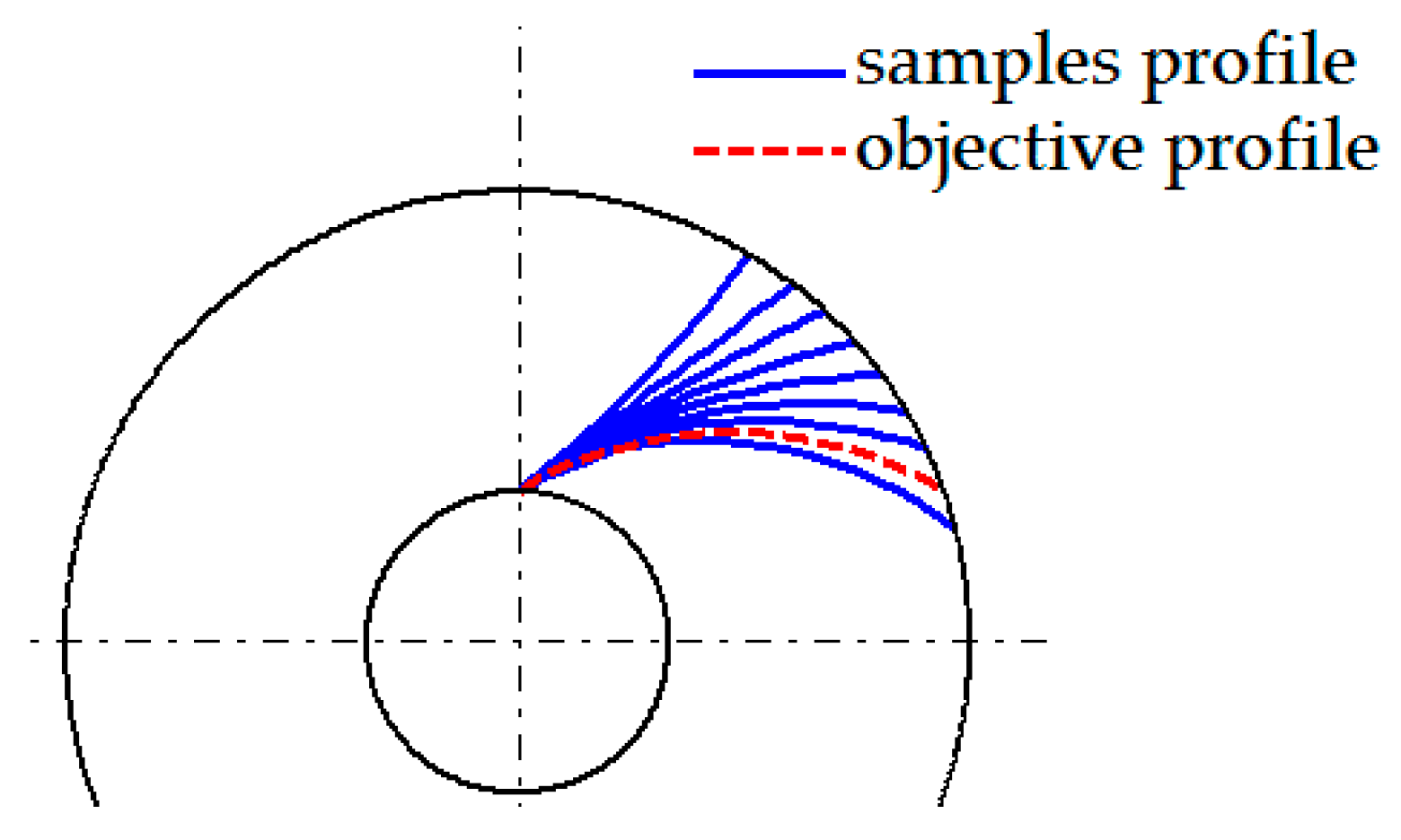
2.3. Parametrization of Blade Profile and Sample Set Generation

The impeller of the model JCP is the cylindrical blade, which can be parameterized by Taylor polynomial and deformed rapidly and efficiently by changing the variable coefficients in the polynomial. The principle of Taylor polynomial to control blade profile is shown in Figure 4, where r is the radius; R1, R2 are the radius of blade inlet and outlet, and θ0, θ are the initial cylindrical angle and cylindrical angle.
A point on the blade profile can be expressed as follows:
f ( r , θ ) = 0 ,
According to the Equation (13), any blade profile can be expressed as a Taylor polynomial based on the original blade profile, as follows:
θ ( r ) = θ 0 + a 1 r 0 + a 2 r 0 2 + + a n r 0 n ,
where r0 is the dimensionless radius and r0 = (RR1)/(R2R1). Equation (13) can be regarded as a Taylor polynomial of the unknown function θ(r) at θ0, so that any blade profile can be expressed by Equation (14).
The impeller blade of the model pump is an equal thickness, so only the pressure face needs to be parameterized, whose equation is as follows:
θ 1 ( r ) = 2.95177 r 5.09806 r 2 + 7.14066 r 3 5.39180 r 4 + 1.64281 r 5
By perturbing the control parameters of Equation (15), the sample set of the blade profile needed by POD reconstruction can be obtained. Blade profiles of eight samples and the objective profile in this research are shown in Figure 5.

2.4. Similar Mesh Reconstruction and Flow Field Interpolation

In this research, the flow field fluctuation intensity corresponding to the objective blade profile was reconstructed and predicted by the basic principle of the Gappy POD method based on the mapping relationship between the geometry and flow field fluctuation intensity of eight samples in the sample set. To ensure the consistency of all data collected from the different samples, structured mesh was employed to each sample impeller with the same rules. If some samples needed to be densified to meet the requirements of computational accuracy and residual convergence to achieve the unification of the grid number, grid deformation technology was employed to reconstruct their grid by referencing a standard grid sample. Then the flow field was interpolated at the reconstructed similar grid nodes, and the vector sets with the same number were obtained.
The dimensionless coordinates of the circumferential angle and radius are defined as εi,j and ηi,j:
ε i , j = ( θ i , j θ i , 1 ) / ( θ i , a θ i , 1 ) ,
η i , j = ( r i , j r i , 1 ) / ( r i , b r i , 1 )
The schematic diagram of the impeller single-channel mesh reconstruction is shown in Figure 6. It uses the same method on blade surface and outlet circumferential surface.

3. Numerical Method

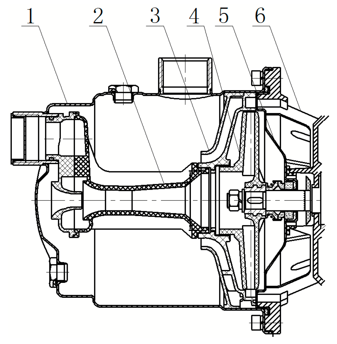
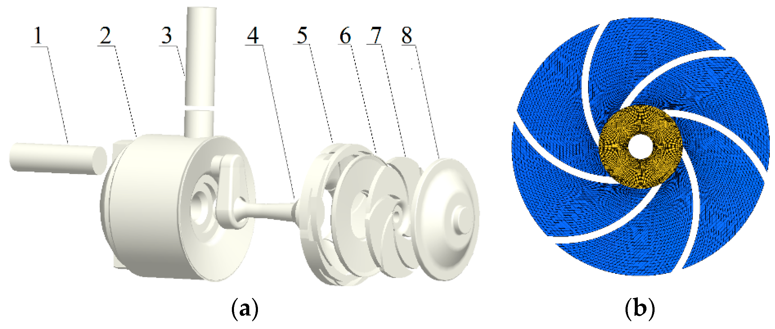
3.1. Physical Model of the Model Jet Centrifugal Pump (JCP)

The rated flow of the model JCP was Q = 2.5 m3/h, rated water head H = 23 m, rated efficiency η = 20%, rotational speed n = 2850 r/min, shaft passing frequency SPF = 47.5 Hz, and blade passing frequency BPF = 285 Hz. The main geometry design parameters of the impeller and guide vane are listed in Table 1.

3.2. Flow Field Calculation Method

The whole computational domain includes impeller, guide vane, jet, front pump cavity, back pump cavity, inlet pipe, outlet pipe, and pump body, which are shown in Figure 7a. ANSYS-ICEM (16.0 ANSYS, Inc., Canonsburg, PA, USA) was employed to the discrete computational domain, hexahedral structured meshes were employed to the computational domain of the impeller and guide vane, and tetrahedral unstructured meshes were employed to other flow-passage components. The number of total meshes was about 3 million after irrelevant checks. The impeller mesh of the model pump is shown in Figure 7b.
CFX (16.0, ANSYS Inc., Pittsburgh, PA, USA) was employed to the flow field calculation. The impeller flow fields were calculated in the rotating coordinate system in the multi-coordinate system, and flow fields of the other components were calculated in the stationary coordinate system. The k-ω turbulence model was adopted, and General Grid Interface (GGI) technology was employed to exchange data between the rotor and stator. The automatic near-wall treatment method was applied to flow near the wall. Pressure inlet and velocity outlet boundary conditions were set, and inlet pressure value was set according to the value obtained from the experiment. All the solid walls were provided with a non-slip wall condition, and roughness was set to 25 μm according to actual processing. The governing equations were solved by the second-order upwind formula and time-term were discretized by the second-order implicit scheme. All residuals were less than 10−5. The time-step was set to 0.000117 s, which means the impeller rotated about 2 degrees per time-step. First, steady calculations were carried out, whose results were taken as the initial value for unsteady calculations. Pressure fluctuation information files of eight rotation cycles on the impeller surface were output for sound field calculations when the flow field showed a stable periodic change.

3.3. Sound Field Calculation Method

In this research, the acoustic finite element method (FEM) was employed to solve the impeller-induced hydrodynamic noise. LMS Virtual.Lab 12.0 was employed to the calculation of sound field, and the wide-band calculation method of fan noise was adopted, which did not need Fourier transform when importing pressure fluctuation data from impeller surface. The impeller was divided into 10 parts to meet the requirement of wavelength and sound source scale and to improve the calculation accuracy. The element length of the acoustic FEM mesh was determined by Equation (18):
L c 6 f max
where c, fmax are the speed of sound and the maximum computational frequency, respectively.
Considering the structural characteristics of the model JCP, the length of the mesh element was given as 8 mm. When the impeller-induced hydrodynamic noise was solved, the surface of other flow-passage components was set as the total reflection wall. That is, it had no transmission of sound on the wall, and the sound only traveled along the water upstream and downstream. The boundary conditions of the inlet and outlet of the pump were defined as the property of total sound absorption. The monitoring point was set at the pump outlet pipe of three times the pipe-diameter.

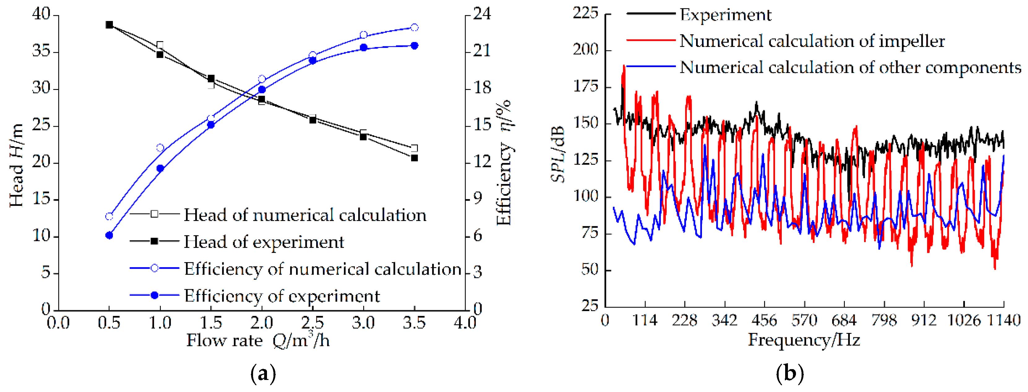
3.4. Numerical Validation

Numerical calculations of flow field and sound field were validated at the JCP test-bed of hydraulic performance and hydrodynamic noise in the Key Laboratory of Fluid Machinery and Systems, Gansu Province. The test system is shown in Figure 8.
The comparison curves of hydraulic performance between the experiment and the numerical simulation is shown in Figure 9a. It can be observed that the variation trend of the performance curve is consistent between numerical calculations and the experiment, and the values at different working points are close. The maximum error of the water head is 4.6%, and efficiency is 4.1% which proves the accuracy of the calculation results.
At the monitoring point, the comparison of frequency response curves of the sound pressure level (SPL) between numerical calculations and the experiment at rated conditions is shown in Figure 9b. It can be observed that the impeller-induced hydrodynamic noise from CFA matches well with the one from the experiment, and the level of the impeller-induced hydrodynamic noise is larger than that of other components in each frequency band. This, therefore, is the main source of the hydrodynamic noise of the JCP. The JCP has several flow-passage components and is complex in structure. It contains mechanical noise and hydrodynamic noise with different characteristics. These different noises may not only be enhanced by overlapping each other but also weakened by subtracting from each other. In addition, the flow field calculation cannot capture the flow separation, secondary flow, vortex, or local slight cavitation completely and accurately. In reality, hydrodynamic noise radiates to the pump outlet after multiple reflections and scatterings on the irregular inner wall. The effects of scattering and transmission on the wall are neglected in the numerical calculations, so the hydrodynamic noise may be increased at some frequencies and inhibited at other frequencies. The sound field numerical calculation method has good accuracy.

4. Reconstruction and Prediction of Flow Field and Sound Field

The flow field fluctuation intensity in the impeller domain and the impeller-induced hydrodynamic noise of the objective sample were reconstructed and predicted by the Gappy POD method based on the mapping relationship among the blade geometry, flow field fluctuation intensity, and impeller-induced hydrodynamic noise of eight samples in the sample set, whose accuracy was validated by comparing it with CFD or CFA results. It includes three parts. First, blade profile parameters and the data of flow field fluctuation intensity of eight samples were given, and the flow field fluctuation intensity corresponding to the objective blade profile was reconstructed. Second, blade profile parameters and the frequency response curves of the SPL of the eight samples were given, and the frequency response curve of the SPL corresponding to objective blade profile was reconstructed. Third, the data of pressure fluctuation intensity and the frequency response curves of the SPL of eight samples were given, and the frequency response curve of the SPL corresponding to objective blade profile was reconstructed.

4.1. Geometry/Flow Field

According to the basic principle of the Gappy POD method described in Section 2.1, the sample vector of the problem is composed of blades profile parameters and the flow field fluctuation intensity data from the similar grid nodes in the impeller.
Flow field fluctuation intensity was reconstructed and predicted, respectively, on the impeller single channel plane, pressure and suction surface of the blade, and impeller outlet circumferential surface. Before reconstructing the flow field, it was necessary to reconstruct the mesh and interpolate the flow field, so that the number of flow field data were unified to 30 × 30 on the single channel plane, 11 × 30 on the pressure and suction surface, and 30 × 11 on the outlet circumferential surface. The number of blade profile parameters were 21 for each sample.

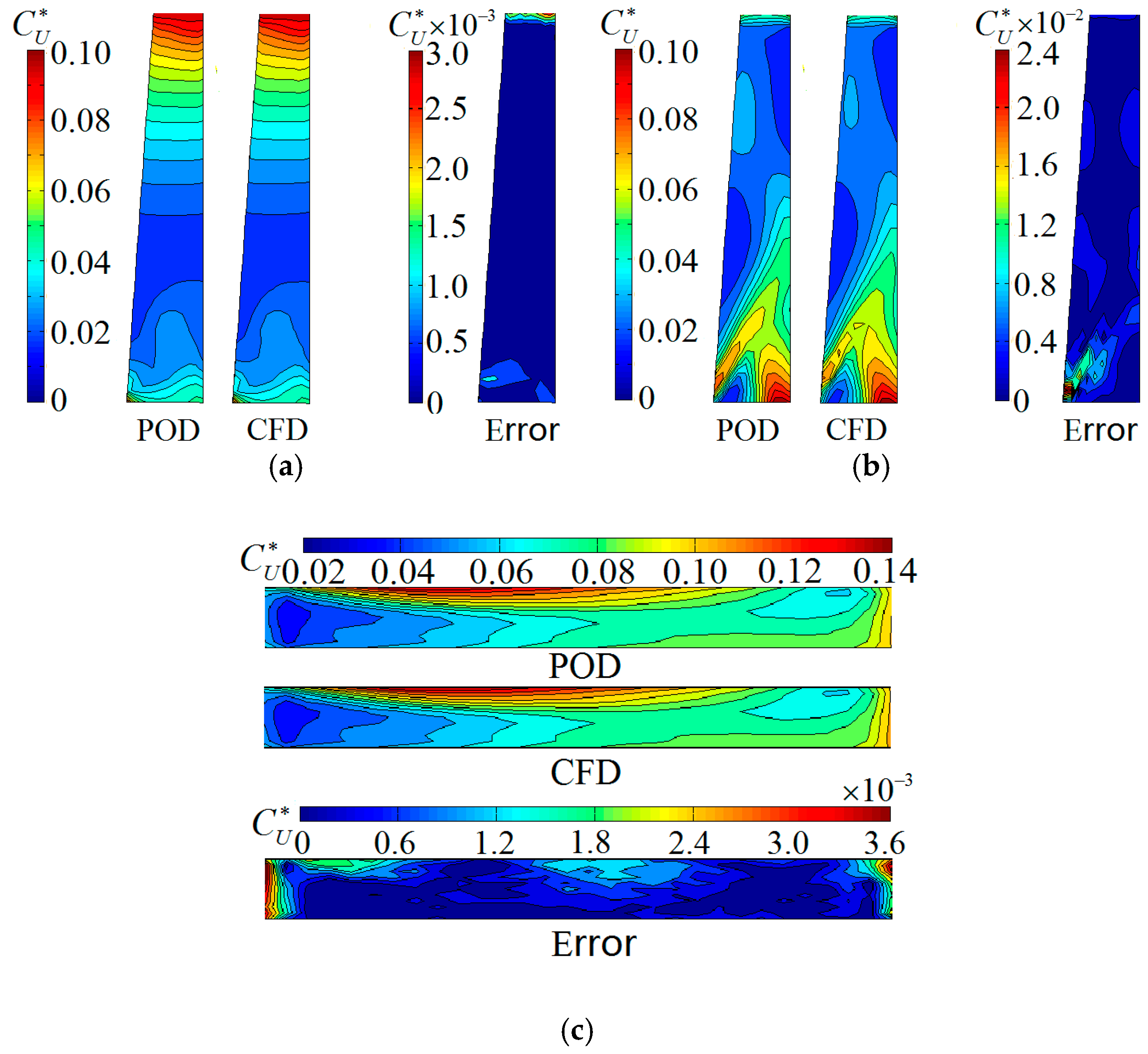
4.1.1. Reconstruction of Pressure Fluctuation Intensity Field

The POD reconstruction, CFD calculation, as well as their error ( Error = | C P _ POD * C P _ CFD * | ) contour of the pressure fluctuation intensity field on the single channel plane are shown in Figure 10. The results from the POD are in good agreement with ones from CFD: The fluctuation intensity increases gradually from the inlet to outlet, and the maximum values appear on the impeller outlet near the pressure surface. Figure 10c shows that the maximum error occurs in the middle of the flow channel and near the suction surface of the impeller outlet.
The POD reconstruction, CFD calculation, and their error contour of the pressure fluctuation intensity field on the pressure and suction surface of the blade, and the outlet circumferential surface of the impeller single channel are shown in Figure 11. The results from the POD are in very good agreement with ones from CFD: On the whole, the pressure fluctuation intensity on the pressure surface is greater than that of suction surface. It increases gradually from the blade inlet to the outlet on the pressure surface. On the suction surface, it changes sharply from large to small on the blade inlet near the hub, then increases gradually with the radius, but decreases near the outlet. Figure 10c shows that the pressure fluctuation intensity changes less from shroud to hub in the axis direction, and it increases first and then decreases from the pressure surface to the suction surface in the circumferential direction. By analyzing the error distribution, it can be found that the maximum error occurs in the middle of the pressure surface, increases gradually from the inlet to the outlet on the suction surface, and has a relatively large area near the blade on the outlet circumferential surface.
By comparing and analyzing the pressure contour of error of the POD reconstruction in each position, it can be observed that the absolute is mainly in the range of 0 to 0.003, and the relative is within 4.0% except for some tiny zone.

4.1.2. Reconstruction of Relative Velocity Fluctuation Intensity Field

The POD reconstruction, CFD calculation, as well as their error contour of the relative velocity fluctuation intensity field on the single channel plane are shown in Figure 12. The distribution and characteristic of the two results are identical: The intensity of the relative velocity fluctuation is weak in the middle of the flow channel. It is much greater than that of other position in the position of the inlet and outlet. This is because the water relative velocity changes sharply and quickly from an axial direction to a circumferential direction in the impeller inlet, and is affected by rotor–stator interaction in the impeller outlet. The error is the most obvious in the area of the channel inlet near the suction surface of blades.
The POD reconstruction, CFD calculation, and their error contour of the relative velocity fluctuation intensity field on pressure and suction surface of the blade, outlet circumferential surface of the impeller single channel are shown in Figure 13. The results from the POD are in very good agreement with the one from CFD: The relative velocity fluctuation intensity decreases first and then increases with the increase of radius on the pressure surface. On the suction surface, the intensity is large in the blade inlet, especially near the hub side. On the outlet circumferential surface, the intensity is larger near the shroud in the axial direction as well as near the pressure surface in the circumferential direction. By analyzing the contour of errors, the maximum error is in the outlet area on the pressure surface and in the inlet area on the suction surface, as well as near the blades side on the outlet circumferential surface.
By comparing and analyzing the relative velocity contour of error of the POD reconstruction in each position, it can be observed that the absolute is mainly in the range of 0 to 0.001, and the relative is within 3.0% except for some tiny zone.

4.1.3. Reconstruction of Turbulent Kinetic Energy Fluctuation Intensity Field

The POD reconstruction, CFD calculation, as well as their error contour of the turbulent kinetic energy fluctuation intensity field on the single channel plane are shown in Figure 14. The results from POD are in very good agreement with ones from CFD: The turbulent kinetic energy fluctuation intensity is weak in the middle of the flow passage and large in at the inlet and outlet. This is due to the same reason as the distribution law of relative velocity fluctuation intensity. Figure 13c shows that the position of the largest error is in the impeller inlet near the pressure surface and in the middle of the passage outlet.
The POD reconstruction, CFD calculation and their error contour of turbulent kinetic energy fluctuation intensity field on pressure and suction surface of the blade, outlet circumferential surface of the impeller single channel are shown in Figure 15. The results from POD are in very good agreement with ones from CFD: The turbulent kinetic energy fluctuation intensity decreases rapidly in the inlet area on the pressure and suction surface, then changes slightly with the increase in radius, and the intensity is large in the middle of the outlet circumferential surface. By analyzing the error distribution, it can be found that the maximum error appears in the inlet area on the pressure surface, in the inlet position near the shroud side on the suction surface, and near the shroud side on the outlet circumferential surface.
By comparing and analyzing the turbulent kinetic energy contour of error of POD reconstruction in each position, it can be observed that the absolute is mainly in the range of 0 to 0.0005, and the relative is within 4.5% except for some tiny zone.
Approximately 1.5 h are needed to complete the calculation of the flow field fluctuation intensity in an impeller rotation period by the CFD method on the workstation with DELLT620, 24 cores and 64 GB memory. However, it only needs 20 s by POD method with the same workstation. This is 1/270 of the time for CFD, so the POD method has very high efficiency.
The above-analyzed results show that the method of Gappy POD has a good accuracy in reconstructing and predicting flow field fluctuation intensity of the objective sample based on the mapping relationship between the geometry and flow field fluctuation intensity of the sample set. The method is employed as a surrogate model to predict the flow field fluctuation intensity in the optimization process of a centrifugal pump impeller, and will significantly reduce the amount and time of numerical calculations of complex flow, improve the optimization efficiency and speed greatly. Because the pressure fluctuation is the main reason of flow-induced noise and vibration of the pump, the prediction of flow field fluctuation intensity by the Gappy POD method, such as pressure fluctuation intensity, can also provide a reference and basis for the noise and vibration characteristics of the models.

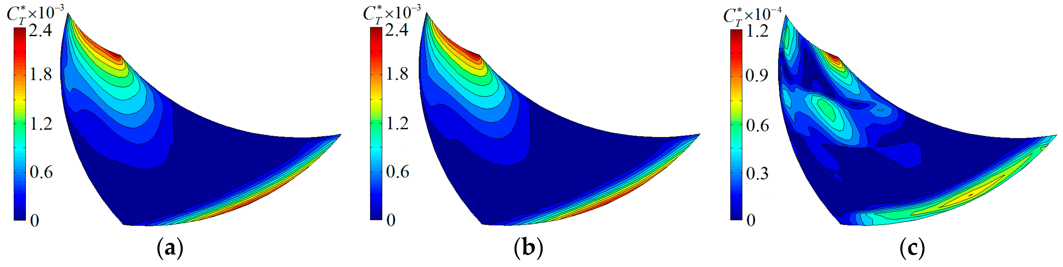
4.2. Geometry/Sound Field

The sample vector of this problem consists of the blade profile parameter and noise data. The noise is expressed by the sound pressure level of impeller-induced hydrodynamic noise in the frequency range of 47.5 Hz to 1140 Hz. The blade profile parameter is 21 data for each sample; and the noise is 1059 data for each sample at the same distance in the spectrum curve.
The POD reconstruction, CFA calculation, as well as their error curve of impeller-induced hydrodynamic noise are shown in Figure 16. The results from the POD are in good agreement with ones from CFA: Both the frequency response curves of SPL obtained by the POD and the CFA method fluctuate taking shaft frequency as the cycle. By analyzing the error distribution of POD prediction and CFA calculation, it can be observed that the absolute error in the different frequency band is within 15 dB and the relative error is within 10%.
The above-analyzed results show that the Gappy POD method is accurate for reconstructing and predicting the impeller-induced hydrodynamic noise of the objective sample based on the mapping relationship between the blades profile parameter and the numerical calculation results of the impeller-induced hydrodynamic noise in the sample set. The numerical simulation of flow-induced noise must be carried out based on the unsteady calculation of the flow field. Therefore, the method could be employed as a surrogate model to predict the acoustic characteristics in the optimization process of a centrifugal pump impeller, which can reduce the computational time for the flow field and sound field, and greatly improve the speed and efficiency of acoustic performance optimization.

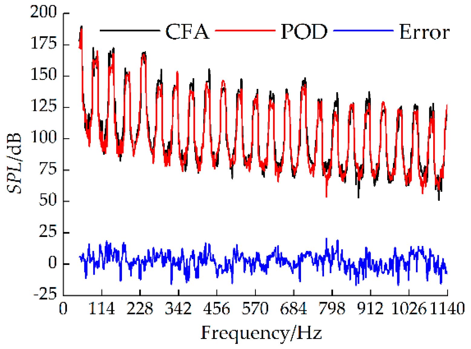
4.3. Flow Field/Sound Field

Dipole noise induced by pressure fluctuation on the wall is the main source of hydrodynamic noise of a centrifugal pump. The magnitude and level of the noise are closely related to the instability of pressure in the time domain. To deeply analyze the mapping relationship between pressure fluctuation intensity field and flow induced-noise field in the impeller domain, the frequency response curve of the SPL of the impeller-induced hydrodynamic noise were reconstructed respectively by the pressure fluctuation intensity data on the pressure and suction surface, and the curve was compared with CFA. The sample vector of this problem consists of the pressure fluctuation intensity data and the SPL data of the impeller-induced hydrodynamic noise in the frequency range of 47.5 Hz to 1140 Hz at the monitoring point.
The POD reconstruction, CFA calculation, as well as their error curves of impeller-induced hydrodynamic noise are shown in Figure 17. The results from POD are in agreement with ones from CFA. By analyzing the error distribution of POD prediction and CFA calculation, it can be observed that the accuracy of using suction surface data is higher than that of the pressure surface. The absolute error is less than 18 dB, and the relative error is less than 12% while using the suction surface data. It is less than 20 dB, and the relative error is less than 15% while using the pressure surface data.
Compared with the results shown in Figure 15 of objective sample reconstruction by mapping relationship of geometry/sound field of the sample set, the errors are larger by mapping relationship of flow field/sound field of the sample set. This is due to the complexity of internal flow of the impeller which makes the formation mechanism of hydrodynamic noise more complex. The noise level is related not only to the intensity of pressure fluctuation in the time domain but also is closely related to the distribution law in the frequency domain. It has some limitations and shortcomings which are due to reconstructing the impeller-induced noise of the objective sample by the method of Section 4.3. The problem needs further consideration and research.

5. Conclusions

The Gappy POD method was proposed to reconstruct and predict the flow field fluctuation intensity in the impeller domain and impeller-induced hydrodynamic noise of the jet centrifugal pump. The sample vectors include blade profile parameter, flow field fluctuation intensity data and sound pressure level parameters.
(1)
The example showed that it has a good accuracy for the reconstruction of the flow field fluctuation intensity and impeller-induced hydrodynamic noise of the objective sample based on the mapping relationship between the geometry and flow field fluctuation intensity of the sample set, or between the geometry and impeller-induced hydrodynamic noise of the sample set. The relative error of the pressure fluctuation intensity field was less than 4.0%, the relative velocity fluctuation intensity field was less than 3.0%, turbulent kinetic energy fluctuation intensity field was less than 4.5%, and impeller-induced hydrodynamic noise was less than 10%.
(2)
It has some limitations and shortcomings due to the reconstruction of the impeller-induced noise of objective sample based on the mapping relationship between the flow field fluctuation intensity and impeller-induced hydrodynamic noise of the sample set. The problem needs further consideration and research.
(3)
The Gappy POD method was employed as a surrogate model to predict the flow field fluctuation intensity and flow-induced noise in the optimization process of a centrifugal pump impeller. It could not only reduce the calculation amount and time significantly and improve optimization speed and efficiency greatly but also could provide a reference for vibration characteristics of the models.

Author Contributions

R.G. and R.Z. wrote the application code of the Gappy POD; R.G. and R.L. performed the experiment; R.G. made the numerical simulation, analyzed the data and wrote the paper.

Funding

This research was funded by Natural Science Foundation of China, grant number 51579125; National Key Research and Development Program of China, grant number 2016YFB0200901.

Acknowledgments

The authors gratefully acknowledge the financial support by the National Natural Foundation of China (51579125), National Key Research and Development Program of China (2016YFB0200901).

Conflicts of Interest

The authors declare no conflict of interest.

References

  1. Wang, Y.; Sun, S.; Yu, B. Acceleration of gas flow simulations in dual-continuum porous media based on the mass-conservation POD method. Energies 2017, 10, 1380. [Google Scholar] [CrossRef]
  2. Fernandezgamiz, U.; GomezMármol, M.; ChacónRebollo, T. Computational modeling of gurney flaps and microtabs by POD Method. Energies 2018, 11, 2091. [Google Scholar] [CrossRef]
  3. Sirovich, L.; Kirby, M. Turbulence and dynamics of coherent structures. Part1: Coherent structures. Q. Appl. Math. 1987, 45, 561–571. [Google Scholar] [CrossRef]
  4. Dolci, V.; Arina, R. Proper orthogonal decomposition as surrogate model for aerodynamic optimization. Int. J. Aerosp. Eng. 2016, 3, 1–15. [Google Scholar] [CrossRef]
  5. Toal, D.J.J.; Bressloff, N.W.; Keane, A.J.; Holden, C.M.E. Geometric filtration using proper orthogonal decomposition for aerodynamic design optimization. AIAA J. 2010, 48, 916–928. [Google Scholar] [CrossRef]
  6. Xiao, M.Y.; Breitkopf, P.; Coelho, R.F.; Villon, P.; Zhang, W.H. Proper orthogonal decomposition with high number of linear constraints for aerodynamical shape optimization. Appl. Math. Comput. 2014, 247, 1096–1112. [Google Scholar] [CrossRef]
  7. Bai, J.Q.; Qiu, Y.S.; Hua, J. Improved airfoil inverse design method based on gappy POD. Acta Aeronaut. ET Astronaut. Sin. 2013, 34, 762–771. [Google Scholar] [CrossRef]
  8. Weiland, C.; Vlachos, P. Analysis of the parallel blade vortex interaction with leading edge blowing flow control using the proper orthogonal decomposition. In Proceedings of the ASME/JSME Joint Fluids Engineering Conference, San Diego, CA, USA, 30 July–2 August 2007. [Google Scholar] [CrossRef]
  9. Eladawy, M.; Heikal, M.; Aziz, A.A.; Siddiqui, M.; Munir, S. Characterization of the inlet port flow under steady-state conditions using piv and pod. Energies 2017, 10, 1950. [Google Scholar] [CrossRef]
  10. Andersson, L.R.; Larsson, A.S.; Hellström, J.G.I.; Andreasson, P.; Andersson, A.G.; Lundström, T.S. Characterization of flow structures induced by highly rough surface using particle image velocimetry, proper orthogonal decomposition and velocity correlations. Engineering 2018, 10, 399–416. [Google Scholar] [CrossRef]
  11. Hall, K.C.; Thomas, J.P.; Dowell, E.H. Proper orthogonal decomposition technique for transonic unsteady aerodynamic flows. AIAA J. 2000, 38, 1853–1862. [Google Scholar] [CrossRef]
  12. Oyama, A.; Nonomura, T.; Fujii, K. Data mining of pareto-optimal transonic airfoil shapes using proper orthogonal decomposition. J. Aircr. 2010, 47, 1756–1762. [Google Scholar] [CrossRef]
  13. Zhang, R.H.; Guo, R.; Yang, J.H.; Li, R.N. Inverse method of centrifugal pump impeller based on proper orthogonal decomposition (POD) method. Chin. J. Mech. Eng. 2017, 30, 1–7. [Google Scholar] [CrossRef]
  14. Zhang, R.H.; Wu, H.; Yang, J.H.; Li, R.N. Reconstruction for gas-liquid flow of liquid-ring pump based on proper orthogonal decomposition. Trans. Chin. Soc. Agric. Mach. 2017, 48, 381–386. [Google Scholar] [CrossRef]
  15. Zhang, R.H.; Chen, X.B.; Guo, G.Q.; Li, R.N. Reconstruction and modal analysis for the flow field of low specific speed centrifugal pump impeller. Trans. Chin. Soc. Agric. Mach. 2018, 11, 1–8. [Google Scholar]
  16. Guo, C.; Gao, M.; Lu, D.Y.; Wang, K. An experimental study on the radiation noise characteristics of a centrifugal pump with various working conditions. Energies 2017, 10, 2139. [Google Scholar] [CrossRef]
  17. Gao, M.; Dong, P.X.; Lei, S.H.; Turan, A. Computational study of the noise radiation in a centrifugal pump when flow rate changes. Energies 2017, 10, 221. [Google Scholar] [CrossRef]
  18. Si, Q.R.; Yuan, S.Q.; Yuan, J.P.; Liang, Y. Investigation on flow-induced noise due to backflow in low specific speed centrifugal pumps. Adv. Mech. Eng. 2013, 6, 631–635. [Google Scholar] [CrossRef]
  19. Liu, H.L.; Dai, H.W.; Ding, J.; Tan, M.G.; Wang, Y.; Huang, H.Q. Numerical and experimental studies of hydraulic noise induced by surface dipole sources in a centrifugal pump. J. Hydrodyn. 2016, 28, 43–51. [Google Scholar] [CrossRef]
  20. Yang, J.; Yuan, S.Q.; Yuan, J.P.; Si, Q.R.; Pei, J. Numerical and Experimental Study on Flow-induced Noise at Blade-passing Frequency in Centrifugal Pumps. Chin. J. Mech. Eng. 2014, 27, 606–614. [Google Scholar] [CrossRef]
  21. Si, Q.R.; Lin, G.; Yuan, S.Q.; Cao, R. Multi-objective optimization on hydraulic design of non-overload centrifugal pumps with high efficiency and low noise. Trans. Chin. Soc. Agric. Eng. 2016, 32, 69–77. [Google Scholar] [CrossRef]
  22. Zhang, J.F.; Jia, J.; Hu, R.X.; Wang, Y.; Cao, P.Y. Flow noise of pipeline pump and bionic sound optimization. Trans. Chin. Soc. Agric. Eng. 2018, 49, 138–145. [Google Scholar] [CrossRef]
  23. Pei, J.; Yuan, S.Q.; Yuan, J.P.; Wang, W.J. Comparative study of pressure fluctuation intensity for a single-blade pump under multiple operating conditions. J. Huazhong Univ. Sci. Technol. Nat. Sci. Ed. 2013, 41, 29–33. [Google Scholar] [CrossRef]
Figure 1. Pictures of impeller and guide vane of the model pump. (a) Guide vane of the jet centrifugal pump (JCP); (b) Impeller of the JCP.
Energies 12 00111 g001
Figure 2. Structural diagram of the model pump. 1: Pump body; 2: Jet; 3: Guide vane; 4: Impeller; 5: Pump cover; 6: Bracket.
Energies 12 00111 g002
Figure 3. Contour of flow field fluctuation intensity. (a) Contour of pressure fluctuation intensity; (b) Relative velocity fluctuation intensity; (c) Turbulent kinetic energy fluctuation intensity.
Energies 12 00111 g003
Figure 4. Schematic diagram of the blade profile while it is controlled by Taylor polynomial.
Energies 12 00111 g004
Figure 5. Schematic diagram of blades profile.
Energies 12 00111 g005
Figure 6. Schematic diagram of mesh reconstruction.
Energies 12 00111 g006
Figure 7. Grid diagram of the impeller and computational domain of model pump. 1: Inlet pipe; 2: Pump body Outlet pipe 3: Outlet pipe; 4: Jet; 5: Guide vane; 6: Front pump cavity; 7: Impeller; 8: Back pump cavity. (a) Computational domain of the model pump; (b) Grid diagram of impeller.
Energies 12 00111 g007
Figure 8. Testing system. (a) Schematic diagram of test system structure; (b) Test site. 1: Valve at pump outlet; 2: Flowmeter; 3: Pressure sensor at pump outlet; 4: Hydrophone at pump outlet; 5: The model pump; 6: Electric motor; 7: Hydrophone at pump inlet; 8: Pressure sensor at pump inlet; 9: Tachometer; 10: Valve at pump inlet; 11: Computer; 12: Oscilloscopes; 13: Measuring instrument of electric power.
Energies 12 00111 g008
Figure 9. Comparison of performances between experiment and numerical calculation. (a) Comparison of hydraulic performance; (b) Comparison of frequency response curves of sound pressure level.
Energies 12 00111 g009
Figure 10. Computational fluid dynamics (CFD) calculation, proper orthogonal decomposition (POD) reconstruction and their error of pressure fluctuation intensity on the single channel plane. (a) POD reconstruction; (b) CFD calculation; (c) Error.
Energies 12 00111 g010
Figure 11. CFD calculation, POD reconstruction, and their error of pressure fluctuation intensity on the blade surface and circumferential surface of impeller outlet. (a) Pressure surface; (b) Suction surface; (c) Circumferential surface of impeller outlet.
Energies 12 00111 g011
Figure 12. CFD calculation, POD reconstruction and their error of relative velocity fluctuation intensity on the single channel plane. (a) POD reconstruction; (b) CFD calculation; (c) Error.
Energies 12 00111 g012
Figure 13. CFD calculation, POD reconstruction, and their error of relative velocity fluctuation intensity on the blade surface and circumferential surface of impeller outlet. (a) Pressure surface; (b) Suction surface; (c) Circumferential surface of impeller outlet.
Energies 12 00111 g013
Figure 14. CFD calculation, POD reconstruction and their error of turbulent kinetic energy fluctuation intensity on the single channel plane. (a) POD reconstruction; (b) CFD calculation; (c) Error.
Energies 12 00111 g014
Figure 15. CFD calculation, POD reconstruction, and their error of turbulent kinetic energy fluctuation intensity on the blade surface and circumferential surface of impeller outlet. (a) Pressure surface; (b) Suction surface; (c) Circumferential surface of impeller outlet.
Energies 12 00111 g015
Figure 16. The POD reconstruction, computational fluid acoustics (CFA) calculation, as well as their error curves of impeller-induced hydrodynamic noise at outlet monitoring point.
Energies 12 00111 g016
Figure 17. The POD reconstruction, CFA calculation, as well as their error curves of impeller-induced hydrodynamic noise at outlet monitoring point. (a) Reconstruction using pressure surface data; (b) Reconstruction using suction surface data.
Energies 12 00111 g017
Table 1. Parameters for the model jet centrifugal pump.
ParameterValue
ImpellerInlet Diameter Dj (mm)40
Outlet Diameter D2 (mm)120
Blade Number Z16
Blade Wrap angle φ (°)78
Blade Outlet width b2 (mm)5.3
Guide vaneBase Diameter (mm)125
Outlet Diameter D3 (mm)64
Blade Number Z25

