Kinetic Study on the Pyrolysis of Medium Density Fiberboard: Effects of Secondary Charring Reactions

Abstract

The reaction models employed in the kinetic studies of biomass pyrolysis generally do not include the secondary charring reactions. The aim of this work is to propose an applicable kinetic model to characterize the pyrolysis mechanism of medium density fiberboard (MDF) and to evaluate the effects of secondary charring reactions on estimated products yields. The kinetic study for pyrolysis of MDF was performed by a thermogravimetric analyzer over a heating rate range from 10 to 40 °C/min in a nitrogen atmosphere. Four stages related to the degradation of resin, hemicellulose, cellulose, and lignin could be distinguished from the thermogravimetric analyses (TGA). Based on the four components and multi-component parallel reaction scheme, a kinetic model considering secondary charring reactions was proposed. A comparison model was also provided. An efficient optimization algorithm, differential evolution (DE), was coupled with the two models to determine the kinetic parameters. Comparisons of the results of the two models to experiment showed that the mass fraction (TG) and mass loss rate (DTG) calculated by the model considering secondary charring reactions were in better agreement with the experimental data. Furthermore, higher product yields than the experimental values will be obtained if secondary charring reactions were not considered in the kinetic study of MDF pyrolysis. On the contrary, with the consideration of secondary charring reactions, the estimated product yield had little error with the experimental data.

1. Introduction

Medium density fiberboard (MDF) is a kind of wood composite material which is widely used in the construction and housing furniture. According to Food and Agriculture Organization (FAO) statistics [1], the total MDF production was more than 100 million m³ over the world in 2017. Specially, in China, the number was more than 59 million m³. A large amount of waste MDF was generated from the need for regular replacement of furniture due to aging, mechanical damage, fire burning, etc. [2]. At the beginning, most of the waste MDF was sent to burn for cooking or space heating, while a small portion was disposed in landfills [3]. With the rapid rising of MDF waste, land occupation and environmental problems are becoming more serious. From the perspective of protecting the natural environment and the sustainable use of resources, it is a good choice to recycle this large amount of waste as energy fuel. Pyrolysis has been proved to be a promising thermochemical conversion technology for resource and energy recovery [4]. On one hand, biomass can be converted into low molecular weight products during the pyrolysis process with low environmental damage. On the other hand, the products generated can be recycled as useful chemicals or gaseous fuels. Hence, it is important to investigate the pyrolysis behavior and pyrolysis kinetics of MDF.

Thermogravimetric analysis (TGA) is widely used to study the pyrolysis behavior of biomass as it is a high-precision method to obtain necessary information to reveal the kinetic mechanism [5,6,7]. Hashim et al. employed TGA to analyze thermal properties of MDF [8]. Additionally, some quantitative methods are usually coupled with TGA curves to determine kinetic parameters, such as model-free methods and model-fitting methods. For example, Yorulmaz et al. calculated the thermal kinetic constants for waste wood samples (including MDF) by using the Coats-Redfern model-fitting method [9]. Han et al. estimated the activation energy of waste MDF by the Ozawa model-free methods [10]. Although these studies may indicate the existence of independent reaction of biomass component, the underlying reaction mechanism is not involved.

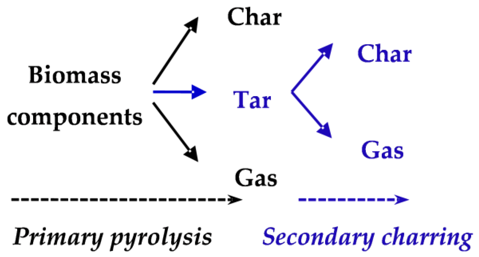
The single biomass component competitive scheme, which was first proposed by Shafizadeh and Chin [11], is commonly used for wood pyrolysis modelling in previous studies. For example, Bastiaans et al. assumed a single reaction to extract Arrhenius parameters and to estimate CO release from MDF [12]. Additionally, competitive schemes for biomass multi-components (cellulose, hemicellulose, and lignin) have also been proposed by Koufopanos et al. [13] and Miller and Bellan [14]. As depicted in Figure 1, for each biomass component, formation of char, tar, and gas complete with each other in the primary pyrolysis. The process of tar to further react to produce more gases and chars is called secondary charring [15]. It is worth noting that this multi-component scheme was never applied in kinetic studies, only the simplified mechanisms of gas and char formation (the black part in Figure 1) were commonly employed in previous studies [16,17,18,19]. Among them, Li et al. determined the kinetic parameters of MDF using the genetic algorithm coupled with Kissinger’s method [19]. However, recently reviews indicate that activation energy for each component calculated using the simplified mechanism varies widely [20,21]. For example, the differences between the reported activation energies of hemicellulose are huge, from about 75 to 225 kJ/mol [15]. The uncertainty estimation of kinetic parameters, which will result in a difference between the estimated product yields and the practical values, may be caused by heating dynamics in the experiment or the absence of secondary charring reactions in the kinetic studies [22]. Lately, some scholars modified the kinetic scheme of biomass pyrolysis to include secondary charring reactions [22,23,24]. However, the kinetic studies on the secondary charring reactions in the multi-component competitive scheme are rare.

In kinetic studies of biomass pyrolysis, the model-free methods and model-fitting methods were usually used to determine kinetic parameters. But, there are several problems with the model-fitting methods, such as the inability to choose the reaction order and the reaction model. The model-free method can only estimate the activation energy at specific conversion rate range for an independent model [25]. Therefore, when analyzing thermogravimetric data coupled with secondary charring reactions, optimization algorithms must be employed to obtain the unknown parameters which cannot be obtained by the above methods. Differential evolution (DE) is an effective method to solve optimization problems in various research fields but rarely used in biomass pyrolysis analysis. Therefore, due to the convergence speed and ease of operation, DE was chosen for data optimization in this study.

The aim of this work is to propose an applicable kinetic model considering secondary charring reactions to better describing the thermal decomposition process of MDF. The differential evolution (DE) algorithm coupled with the proposed model was used to obtain the reaction kinetics of MDF pyrolysis and the effects of secondary charring reactions on products yields were also evaluated.

2. Experimental and Kinetic Modeling

2.1. Experimental

2.1.1. MDF Sample

MDF used in this work came from a wood factory in Hefei City, Anhui Province, China. According to the manufacturer, the main component of the MDF is pine fiber. At first, the MDF was milled, and then the particles with a size less than 125 μm were obtained through a series of Tyler sieves. The samples were dehydrated for at least 48 hours in an XGQ-2000 (BAIHUI, Dongguan, Guangdong, China) electric drying oven at 105 °C, and then sealed in plastics bags in preparation for following tests. According to ASTM standards, proximate analysis was performed using a LECO TGA 701thermogravimetric analyzer. Ultimate analysis was performed using a LECO TruSpec CHN to detect carbon, hydrogen, and nitrogen. Sulfur was detected using a LECO TruSpec S. The proximate and ultimate analysis results of MDF sample are shown in

Table 1. Proximate and ultimate analysis of MDF sample.

Feedstock	Proximate Analysis (wt %)				Ultimate Analysis (wt %)
MDF	Moisture	Ash	Volatiles	Fixed carbon	C	H	O a	N	S
-	8.28	4.69	81.2	5.83	44.96	6.26	44.87	3.35	0.56

^a By difference.

.

2.1.2. TGA Tests

Thermogravimetric analysis was carried out using a NETZSCH STA 449 F3 Jupiter (NETZSCH, Selb, Germany) thermal analyzer. The samples of 6 ± 0.5 mg were heated with a gas flow rate of 80 mL/min under a nitrogen atmosphere. The program temperature was increased from room temperature to about 800 °C at four selected heating rates of 10, 20, 30, and 40 °C /min. The real-time mass change and heat flux change were monitored using software in the whole process. TGA experiments were repeated three times and the results showed a good repeatability (mean uncertainly is less than 1%).

2.2. Kinetic Modeling

2.2.1. Kinetic Reaction Model

As illustrated in Section 1, lignocellulosic biomass can be considered to be composed of n components. In this work, the MDF sample is made by pine and less than 10% resin. Therefore, the independent reactions of four components: resin, hemicellulose, cellulose, and lignin, are applied to explain the decomposition of MDF.

Table 2. Two kinetic models to explain the decomposition of MDF applied in this work.

Model I		Model II
1 *:	$\mathrm{resin}\to {\upsilon }_{r}gases+{\phi }_{r}char$	1 *:	$\mathrm{resin}\to {\gamma }_{r}tar+{\delta }_{r}gases+{\sigma }_{r}char$
	$\mathrm{hemicellulose}\to {\upsilon }_{h}gases+{\phi }_{h}char$		$\mathrm{hemicellulose}\to {\gamma }_{h}tar+{\delta }_{h}gases+{\sigma }_{h}char$
	$\mathrm{cellulose}\to {\upsilon }_{c}gases+{\phi }_{c}char$		$\mathrm{cellulose}\to {\gamma }_{c}tar+{\delta }_{c}gases+{\sigma }_{c}char$
	$\mathrm{lignin}\to {\upsilon }_{l}gases+{\phi }_{l}char$		$\mathrm{lignin}\to {\gamma }_{l}tar+{\delta }_{l}gases+{\sigma }_{l}char$
		2 *:	$\mathrm{tar}\to \tau gases+\theta char$

* 1 and 2 represents the primary pyrolysis and secondary charring reaction, respectively.

lists the two models applied in this study detailed (Model II and Model I represent the models that considering the secondary charring reactions or not, respectively).

For the convenience of writing, some parameters are listed here. f(α) is the conversion function that describes the reaction mechanism, g(α) is the integrated forms of f(α); m₀, m_t, and m_∞ represent the initial, instantaneous, and the final solid mass of samples, respectively; the kinetic triplets A is the pre-exponential factor, E is the activation energy and n is the reaction order; R is the gas constant; for component i, W_i is the instantaneous mass fraction, W_i,0 is the initial mass fraction, γ_i, σ_i, and φ_i are the stoichiometry coefficient of tar and char, respectively.

It is known that the kinetic parameters of thermogravimetry can be effectively calculated based on the decomposition rate dα/dt which is assumed to be a function of temperature T and the degree of conversion α [26,27]:

$$\frac{d\alpha }{dt}=k\left(T\right)f\left(\alpha \right),$$

(1)

The conversion rate can be described as $\alpha =\left(m_0-m_t\right)/\left(m_0-m_{\infty }\right)$, and the kinetic constant of temperature k(T) is expressed by Arrhenius equation as $k\left(T\right)=Aexp\left(-E/RT\right)$.

The associated kinetic equations of models can be expressed as follows:

• Model I

The reaction rate for reactions in Model I can be calculated by:

$$\frac{d{W}_i}{dt}=-A_{i}exp\left(-\frac{E_i}{RT}\right)W_{i,0}{\left(\frac{W_i}{W_{i,0}}\right)}^{n_i},$$

(2)

$$\frac{d{\alpha }_i}{dt}=A_{i}exp\left(-\frac{E_i}{RT}\right){\left(1-{\alpha }_i\right)}^{n_i},$$

(3)

The total mass loss rate (dW/dt)_tot and the total solid mass fraction W_tot can be calculated as:

$${\left(\frac{dW}{dt}\right)}_{tot}={\displaystyle \sum _i^n}(\frac{d{W}_i}{dt}+\frac{d{W}_{char,i}}{dt})={\displaystyle \sum _i^n}(\frac{d{W}_i}{dt}+{\phi }_i{W}_{i,0}\frac{d{\alpha }_i}{dt}),$$

(4)

$$W_{tot}=1-{\displaystyle \sum _i^n}\left(1-{\phi }_i\right){\alpha }_i{W}_{i,0},$$

(5)

• Model II

Step 1 (primary pyrolysis):

Similar to Model I, the mass loss rate (dW/dt)₁ and the solid mass fraction W₁ of step 1 can be calculated as:

$${\left(\frac{dW}{dt}\right)}_1={\displaystyle \sum _i^n}(\frac{d{W}_i}{dt}+{\sigma }_i{W}_{i,0}\frac{d{\alpha }_i}{dt}),$$

(6)

$$W_1=1-{\displaystyle \sum _i^n}\left(1-{\sigma }_i\right){\alpha }_i{W}_{i,0},$$

(7)

Step 2 (secondary charring reaction):

The reaction rate for secondary charring reaction can be calculated by:

$$\frac{d{W}_{tar}}{dt}=-A_{tar}exp\left(-\frac{E_{tar}}{RT}\right)W_{tar,0}{\left(\frac{W_{tar}}{W_{tar,0}}\right)}^{n_{tar}},$$

(8)

$$\frac{d{\alpha }_{tar}}{dt}=A_{tar}exp\left(-\frac{E_{tar}}{RT}\right){\left(1-{\alpha }_{tar}\right)}^{n_{tar}},$$

(9)

where W_tar,0 is the initial mass fraction of tar which is calculated from step 1:

$$\frac{d{W}_{tar,0}}{dt}={\displaystyle \sum _i^n}{\gamma }_i{W}_{i,0}\frac{d{\alpha }_i}{dt},$$

(10)

Therein, W_tar, A_tar, E_tar, n_tar denote the instantaneous mass fraction the kinetic triplets for tar generated by step 1, respectively.

Thus, the mass of char generated by step 2 W_char,2 is calculated as:

$$\frac{d{W}_{char,2}}{dt}=\theta W_{tar,o}\frac{d{\alpha }_{tar}}{dt},$$

(11)

where θ is the coefficient of char in step 2.

Therefore, the total solid mass fraction in the whole process can be expressed as:

$$W_{tot}=W_1+W_{char,2},$$

(12)

The total mass loss rate of whole process is then deduced as:

$${\left(\frac{dW}{dt}\right)}_{tot}={\displaystyle \sum _i^n}(\frac{d{W}_i}{dt}+{\sigma }_i{W}_{i,0}\frac{d{\alpha }_i}{dt})+\theta W_{tar,o}\frac{d{\alpha }_{tar}}{dt},$$

(13)

2.2.2. Optimization Method—Differential Evolution Algorithm

Differential evolution (DE) is originally proposed by Rainer Storn and Kenneth Price, in 1995 [28]. It is a kind of population-based adaptive global optimization algorithm. Assuming there are M individuals in a random population. An individual consists of n-dimensional vectors, which can be expressed as $X_i\left(g\right)=\left(x_{i,1}\left(g\right),x_{i,2}\left(g\right),\dots x_{i,n}\left(g\right)\right),i=1,2,\dots ,M;g=1,2,\dots ,N$. N is the maximum number of iterations. In the present study, one unknown parameter, such as the activation energy E, is an individual. The implementation of DE is as follows [29]:

• Initialization

The value of the jth dimension of the ith individual is calculated as:

$$x_{ij}\left(g\right)=x_{ij}^L+rand\left(0,1\right)\left(x_{ij}^U-x_{ij}^L\right),$$

(14)

where $x_{ij}^L$, $x_{ij}^U$ denote the lower and upper bands of the ith individual, respectively. rand (0, 1) denotes a random number distributed in [0, 1].

• Variation

A variation individual is calculated via three random individuals:

$$h_{ij}\left(g\right)=x_{r1j}+F\left(x_{r2j}-x_{r3j}\right),r1\ne r2\ne r3\ne i,$$

(15)

where F is the scaling factor.

• Crossover

The new individual can be calculated as:

$$v_{ij}\left(g\right)=\{\begin{array}{c}{h}_{ij}\left(g\right),rand\left(0,1\right)\le Cr\\ x_{ij}\left(g\right),rand\left(0,1\right)>Cr\end{array},$$

(16)

where Cr is the cross rate distributed in [0, 1].

• Selection

In this step, the individual in the next iteration is selected by:

$$X_i\left(g+1\right)=\{\begin{array}{cc}{V}_i\left(g\right),\hfill & \hfill f\left(V_i\left(g\right)\right)<f\left(X_i\left(g\right)\right)\\ X_i\left(g\right),\hfill & \hfill else\end{array},$$

(17)

where f(x) is the fitness of the individuals. In the present study, the fitness is evaluated by the objective function obj, which can be calculated as:

$$obj={\displaystyle \sum _1^k}c\frac{{\sum }_1^{n_j}\left|W_{tot,j}-W_{exp,j}\right|}{{\sum }_1^{n_j}{W}_{exp,j}}+{\displaystyle \sum _1^k}\left(1-c\right)\frac{{\sum }_1^{n_j}\left|{\left(\frac{dW}{dt}\right)}_{tot,j}-{\left(\frac{dW}{dt}\right)}_{exp,j}\right|}{{\sum }_1^{n_j}{\left(\frac{dW}{dt}\right)}_{exp,j}},$$

(18)

where W_tot and (dW/dt)_tot are the calculated solid mass and mass loss rate in the pyrolysis process, respectively. exp means the corresponding experimental data. n_j is the number of data points considered in each single heating rate and k is the number of heating rates. c is the weight coefficient, and c = 0.5 is set for equally weighted both mass and mass loss rate.

From the objective function, there are 28 unknown parameters in Model II: kinetic triplets (E_i, A_i, n_i), initial mass fractions (W_i,0), tar yields (γ_i), and char yields (σ_i, θ) for each component and tar. Since the initial mass fraction of the sum of the four components is equal to 1, the initial mass fraction of lignin can be calculated by W_l,0 = 1 − W_r,0 − W_h,0 − W_c,0. Then the number of unknown variables is 27. So, there are 27 individuals in Model II and 19 in Model I. In order to obtain the optimal solution, appropriate algorithm parameters should be set. In this work, the population size, scaling factor, crossover probability and maximum iteration number of the optimization are set as 60, 0.5, 0.2, and 1000, respectively. The optimization process is implemented in MATLAB.

2.2.3. Estimation of Initial Guesses of Model Parameters for DE

If an appropriate initial guess of unknown variable is provided, the DE optimization efficiency can be greatly improved. Therefore, the kinetic triplets are firstly estimated prior to the optimization process.

The complementary use of model-free and model-fitting methods were suggested by Khawam and Flanagan [30] to determine solid state reaction kinetic triplets from experimental data. In this study, three model-free kinetic methods (Equations (21)–(23)) [31,32,33] and one model-fitting method (Equation (24)) [34,35] were used to estimate the kinetic triplets.

Flynn-Wall-Ozawa (FWO):

$$\ln \beta =\ln \left(\frac{A_{\alpha }{E}_{\alpha }}{Rg\left(\alpha \right)}\right)-5.331-1.052\left(\frac{E_{\alpha }}{R{T}_{\alpha }}\right),$$

(19)

Starink:

$$\ln \left(\frac{\beta }{T_{\alpha }^{1.92}}\right)=\ln \left(\frac{A_{\alpha }{E}_{\alpha }}{Rg\left(\alpha \right)}\right)-0.312-1.0008\left(\frac{E_{\alpha }}{R{T}_{\alpha }}\right),$$

(20)

Kissinger-Akahira-Sunose (KAS):

$$\ln \left(\frac{\beta }{T_{\alpha }^2}\right)=\ln \left(\frac{A_{\alpha }{E}_{\alpha }}{Rg\left(\alpha \right)}\right)-\frac{E_{\alpha }}{R{T}_{\alpha }},$$

(21)

Coats-Redfern (CR):

$$\ln \left(\frac{g\left(\alpha \right)}{T_{\alpha }^2}\right)=\ln \left(\frac{A_{\alpha }R}{E_{\alpha }\beta }\right)-\frac{E_{\alpha }}{R{T}_{\alpha }},$$

(22)

It is noted that model-free methods can calculate the kinetic parameters without equation expression of g(α).

The kinetic models used in this study were presented in Section 2.2. THE optimization methodology (DE) was introduced for the estimation of kinetic parameters. Moreover, to improve the DE optimization efficiency, three model-free kinetic methods and one model-fitting method were presented for the initial guesses of the kinetic triplets.

3. Results and Discussion

3.1. Thermogravimetric Analysis

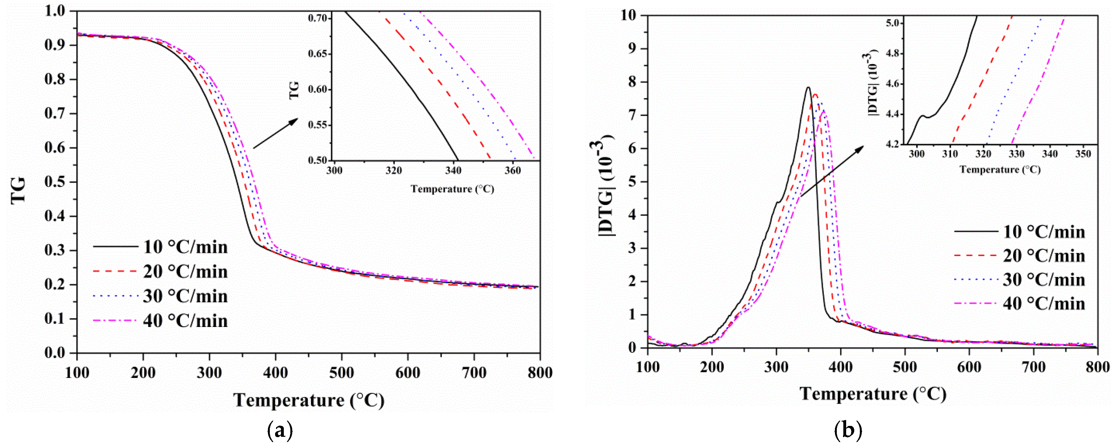
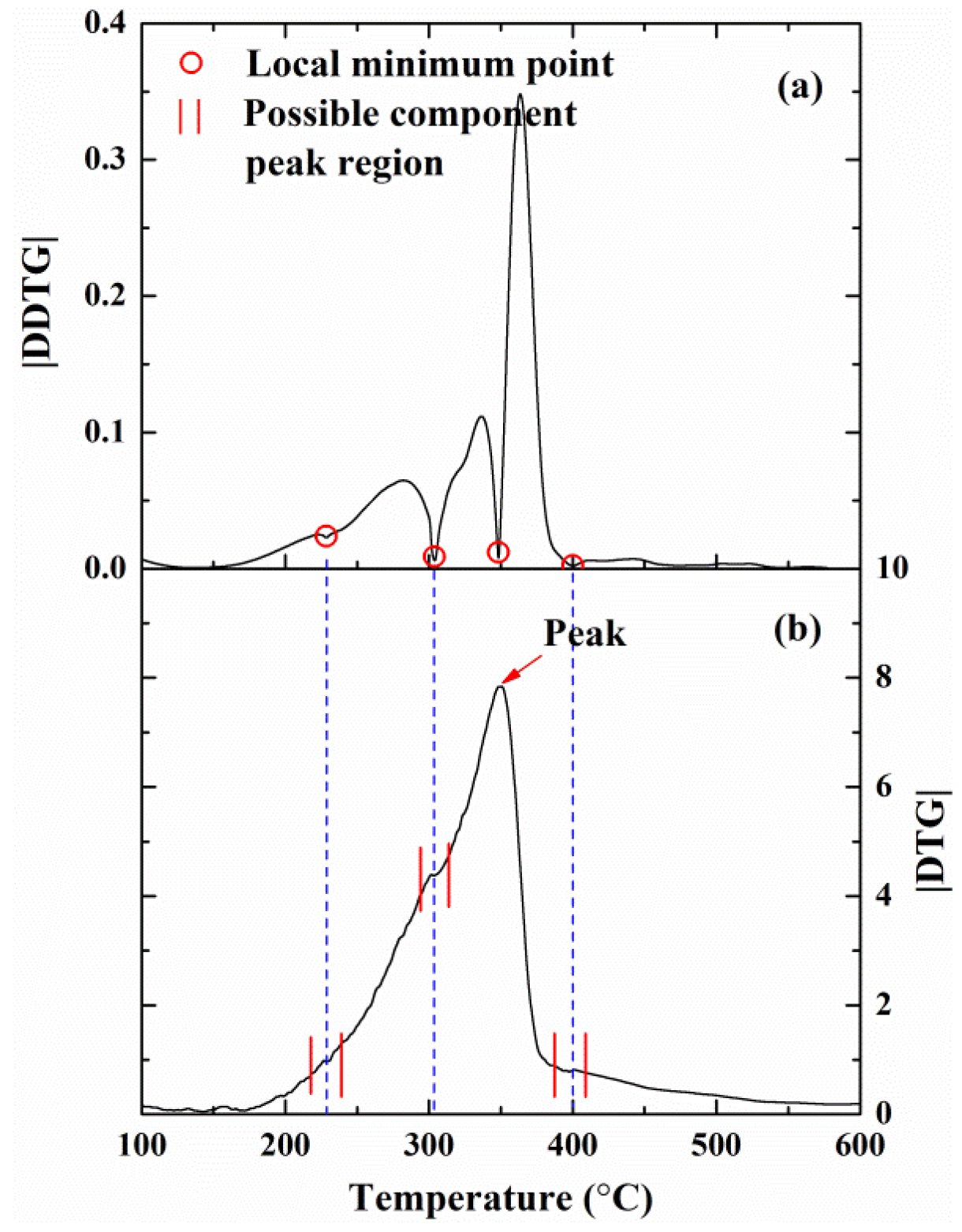
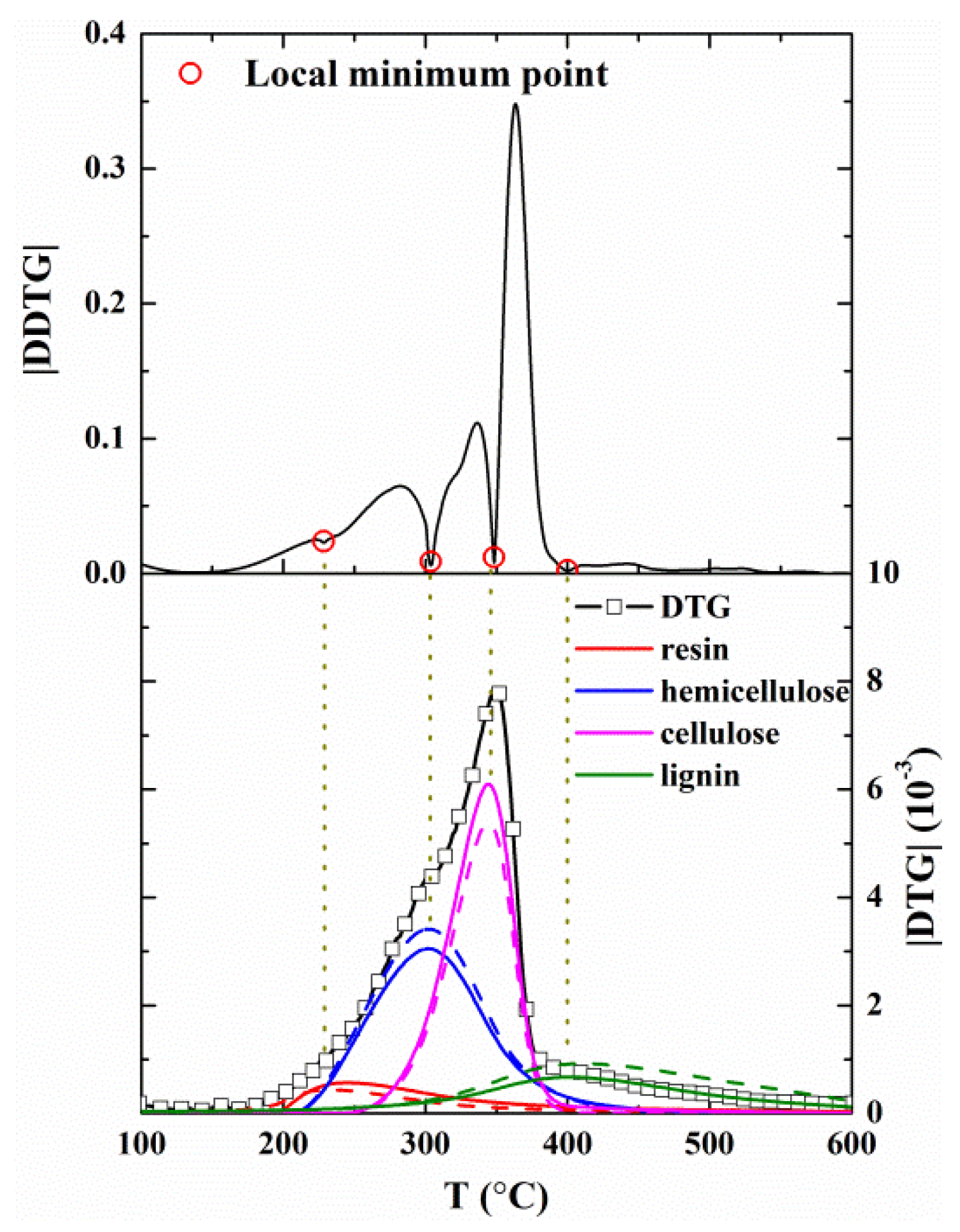
The mass fraction (TG) and mass loss rate (DTG) profiles in the cases of 10, 20, 30, and 40 °C/min are illustrated in Figure 2. As shown in Figure 2a, a similar phenomenon occurs in any thermogravimetric analysis can be observed: a shift of the TG curves at higher temperature happens by the increase of the heating rate. In Figure 2b, there are less identifiable inflection points in the |DTG| curves. Li et al. [19] estimated the possible components and sub-reactions by comparing DTG and DDTG (the second derivatives of TG curves). Figure 3 illustrates the corresponding |DTG| and |DDTG| curves at 10 °C/min. There are four local minimum values in the |DDTG| curve, which correspond to the possible peak DTG of each sub-reaction. This phenomenon can also be observed for other heating rates. Therefore, four components are expected to react in the pyrolysis process of MDF. The temperatures corresponding to the peak DTG of each component may be 228, 303, 368, and 400 °C.

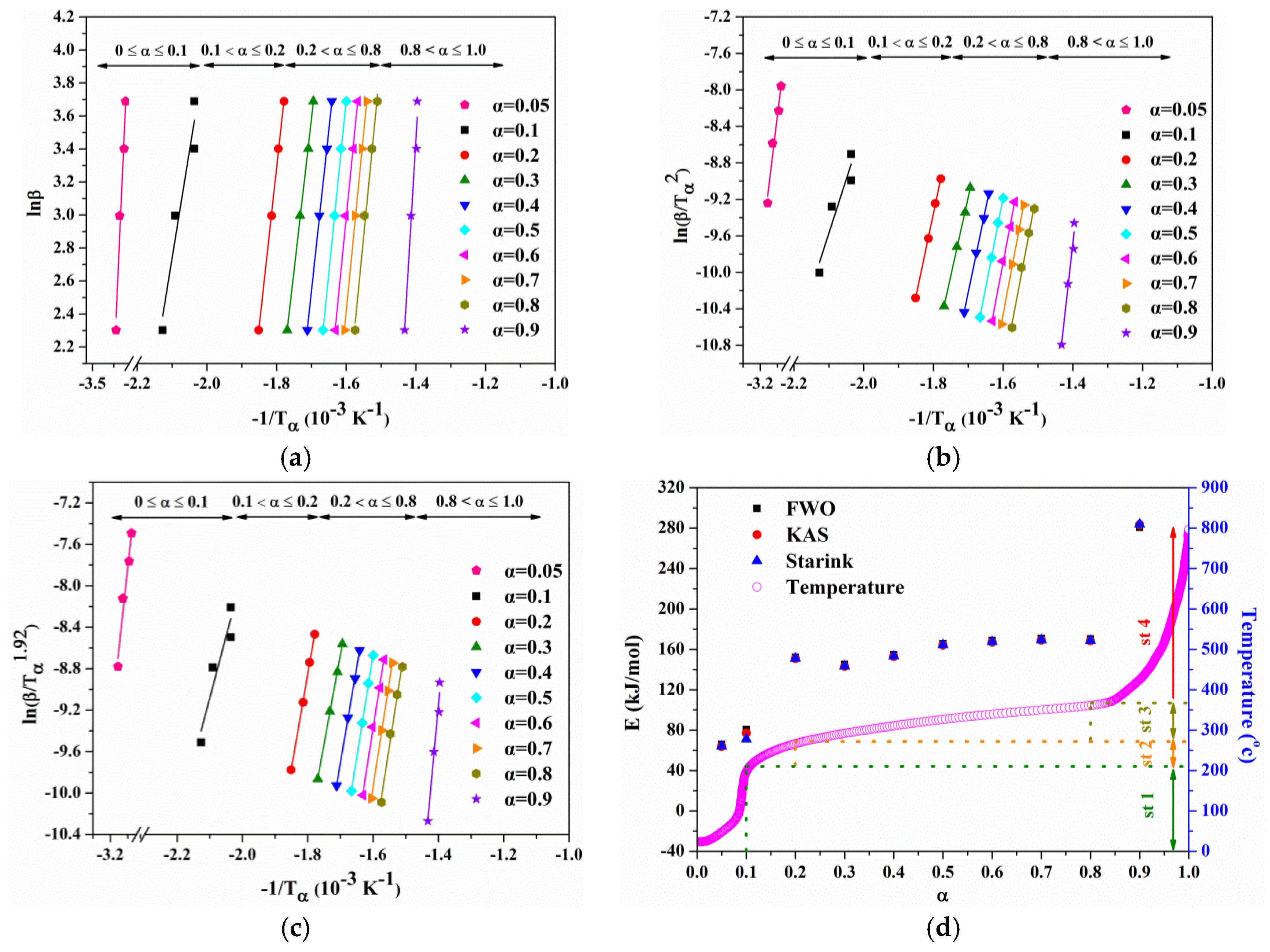
Based upon Section 2.2.3., the Arrhenius plots for the conversion from 0.1 to 0.9 by model-free models FWO, Starink and KAS are shown in Figure 4a–c, respectively. Differences appear at α = 0.1, α = 0.2, and α = 0.8. The activation energies at different conversion obtained from the slopes of plots are presented in Figure 4d and

Table 3. Calculation results of E by FWO, KAS and Starink methods and evaluation values of lnA.

α	FWO		KAS		Starink		Average Value
	E (kJ/mol)	R2	E (kJ/mol)	R2	E (kJ/mol)	R2	E (kJ/mol)	lnA	R2
0.05	65.94	0.96	63.89	0.95	64.06	0.95	64.63	22.82	0.95
0.1	80.66	0.90	70.06	0.86	71.19	0.86	76.30	24.81	0.87
0.2	152.10	0.99	150.86	0.99	151.10	0.99	151.36	37.62	0.99
0.3	145.11	0.99	143.06	0.99	143.33	0.99	143.84	36.33	0.99
0.4	154.83	0.99	152.97	0.99	153.24	0.99	153.68	38.01	0.99
0.5	165.71	0.99	164.15	0.99	164.43	0.99	164.77	39.90	0.99
0.6	168.79	0.99	167.17	0.99	167.45	0.99	167.80	40.42	0.99
0.7	170.73	0.99	169.04	0.99	169.32	0.99	169.70	40.74	0.99
0.8	170.30	0.99	168.38	0.99	168.68	0.99	169.12	40.65	0.99
0.9	280.67	0.97	283.51	0.96	283.75	0.96	282.64	60.01	0.96
Mean value (0.05–0.1)	73.30	0.93	66.98	0.90	67.63	0.91	69.30	23.82	0.92
Mean value (0.1–0.2)	116.38	0.95	110.46	0.93	111.15	0.93	112.66	31.21	0.94
Mean value (0.2–0.8)	160.08	0.99	159.38	0.99	159.65	0.99	159.70	39.10	0.99
Mean value (0.8–0.9)	225.49	0.98	225.95	0.98	226.22	0.98	225.88	50.33	0.98

. High correlation coefficients R² of fitting curves at different conversions are demonstrated. The values of E at each conversion determined by different model-free methods are almost the same. In addition, the values of E increase gradually at 0 ≤ α ≤ 0.1, followed by a sharp increase at 0.1 < α ≤ 0.2. Then E remains almost constant at 0.2 < α ≤ 0.8. Finally, a second sharp increase of E occurs at 0.8 < α ≤ 1.0. These ranges are coincidence with the position where the differences observed in Figure 4a–c. Therefore, four stages which related to four sub-reactions of four components can be divided in the pyrolysis process by α = 0.1, α = 0.2 and α = 0.8.

In Figure 4d, the temperatures corresponding to the four stages can be observed.

Table 4. Pyrolysis process based upon conversion and temperature at different heating rates.

Heating Rate (°C/min)	First Stage α/T (°C)	Second Stage α/T (°C)	Third Stage α/T (°C)	Forth Stage α/T (°C)
10	0–0.1/25–214	0.1–0.2/214–274	0.2–0.8/274–363	0.8–1.0/363–800
20	0–0.1/25–220	0.1–0.2/220–285	0.2–0.8/285–375	0.8–1.0/375–800
30	0–0.1/25–231	0.1–0.2/231–292	0.2–0.8/292–382	0.8–1.0/382–800
40	0–0.1/25–234	0.1–0.2/234–296	0.2–0.8/296–389	0.8–1.0/389–800

lists the pyrolysis process based upon conversion and temperature at different heating rates. In the case of 10 °C/min, the first stage in the range of 25–214 °C refers mainly to the degradation of resin [19,36]. The second stage of 214–274 °C corresponds to the degradation of hemicellulose [36]. The third stage in the range of 274–363 °C is attributed to the decomposition of cellulose [37]. Finally, the last stage, temperatures above 363 °C, is mainly dominated by the decomposition of lignin [38]. These stages are comparable to the analysis of resin, hemicellulose, cellulose, and lignin found in [19] and [39].

3.2. Estimated Initial Guess of Model Parameters

It is known that the activation energy which is related to the reaction rate represents the minimum energy required to start a reaction. Therefore, a large change of activation energy against conversion corresponds to the occurrence of several reactions [31,40]. As shown in Figure 4d, E remains almost constant at 0.2 < α ≤ 0.8 whereas it increases significant in other ranges. Thus, the pyrolysis process at 0.2 < α ≤ 0.8 may be expressed by a single reaction model g(α), as listed in

Table 5. Calculation values of E based on the CR method for 0.2 ≤ α ≤ 0.8.

Reaction Model [29,41]		10 °C/min		20 °C/min		30 °C/min		40 °C/min		Mean Value
		E (kJ/mol)	R2	E (kJ/mol)	R2	E (kJ/mol)	R2	E (kJ/mol)	R2	E (kJ/mol)	R2
Reaction order
0th-order	g(α) = α	32.83	0.99	35.13	0.99	34.06	0.99	33.43	0.99	33.86	0.99
1st-order	g(α) = −ln(1 − α)	66.67	0.99	70.92	0.99	69.01	0.99	68.20	0.99	68.7	0.99
2nd-order	g(α) = [1 − (1 − α)−1)]/( −1)	115.9	0.98	122.96	0.98	119.8	0.97	118.81	0.98	119.37	0.98
3rd-order	g(α) = [1 − (1 − α)−2)]/( −2)	178.58	0.97	189.23	0.97	184.49	0.96	183.24	0.98	183.88	0.97
4th-order	g(α) = [1 − (1 − α)−3)]/( −3)	250.5	0.96	265.3	0.96	258.65	0.95	257.24	0.97	257.92	0.96
Diffusional
1-D	g(α) = α2	75.91	0.99	80.73	0.99	78.73	0.99	77.57	0.99	78.23	0.99
2-D	g(α) = (1 − α)ln(1 − α)+α	93.87	0.99	99.68	0.99	97.19	0.99	95.94	0.99	96.67	0.99
3-D (Jander)	g(α) = [1 − (1 − α)1/3]2	117.64	0.99	124.71	0.99	121.8	0.99	120.47	0.99	121.16	0.99
GB	g(α) = 1 − 2/3α− (1 − α)2/3	101.6	0.99	107.92	0.99	105.34	0.99	104.01	0.99	104.71	0.99
Nucleation
2/3-Power law	g(α) = α3/2	54.37	0.99	57.95	0.99	56.37	0.99	55.45	0.99	56.04	0.99
2-Power law	g(α) = α1/2	11.28	0.98	12.34	0.99	11.74	0.99	11.37	0.98	11.68	0.99
3-Power law	g(α) = α1/3	4.07	0.95	4.74	0.98	4.32	0.95	3.99	0.92	4.28	0.95
2-AE	g(α) = [−ln(1 − α)]1/2	28.18	0.99	30.26	0.99	29.18	0.98	28.77	0.99	29.10	0.99
3-AE	g(α) = [−ln(1 − α)]1/3	15.38	0.99	16.63	0.99	15.96	0.98	15.63	0.99	15.90	0.99
4-AE	g(α) = [−ln(1 − α)]1/4	8.97	0.98	9.89	0.99	9.31	0.96	9.03	0.99	9.30	0.98
Contracting geometry
Area	g(α) = 1 − (1 − α)1/2	47.89	0.99	51.05	0.99	49.55	0.99	48.89	0.99	49.34	0.99
Volume	g(α) = 1 − (1 − α)1/3	53.71	0.99	57.20	0.99	55.62	0.99	54.87	0.99	55.35	0.99

. The activation energies calculated by the slopes of CR plots coupled with 17 types of reaction models are listed in Table 5.

According to Chen et al. [31], if the mean value of activation energies for different heating rates at 0.2 < α ≤ 0.8 based upon one certain model is most close to the value by the model-free methods, then this model may dominate the reactions in this stage. As a result, the average value of E at 0.2 < α ≤ 0.8 based upon the 3rd-order reaction model g(α) = [1 − (1 − α)⁻²)]/(−2) (183.88 kJ/mol) is closest to the value by the model-free methods (159.70 kJ/mol, as shown in Table 3). Thus, the 3rd-order reaction model may be the most appropriate model to express the pyrolysis process in the range of 0.2 < α ≤ 0.8.

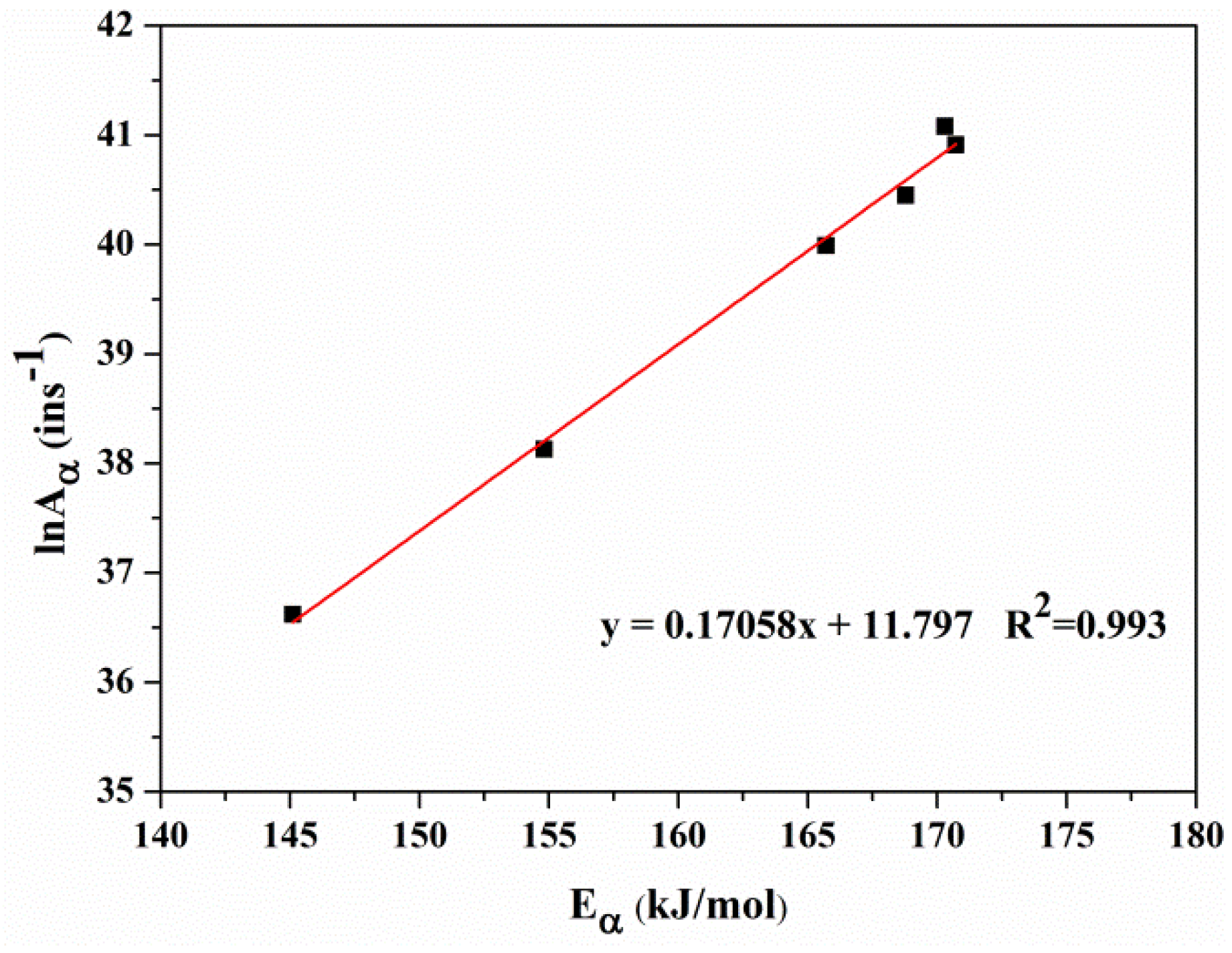
Since the higher correlation coefficients R², the E_α obtained by FWO are used to determine the pre-exponential factor. The lnA_α values evaluated by FWO with the 3rd-order reaction model are plotted in Figure 5. It can be seen that lnA_α varies with E_α, and a fitting line which shows the so-called kinetic compensation effect [41] can be obtained: $\ln A_{\alpha }=0.17058E_{\alpha }+11.797,R^2=0.993$. According to Yao et al. [42], if a compensation effect is observed, the choice of 3rd-order reaction model is appropriate. At the same time, the compensation effect parameters, a = 0.17058 and b = 11.797, can describe the whole pyrolysis process well for that they are not affected by experimental conditions [43]. Thus, the evaluations of lnA_α based upon the compensation effect are listed in Table 3. The mean values of E and lnA of the four stages will be used as the initial guesses for the optimization process below.

3.3. Model Parameter Optimization by DE

The optimized parameters of the two models are listed in

Table 6. Optimized values of kinetic parameters for Model I and Model II by DE.

Component	Parameter	Initial Guess	Range	Model I Optimized Value	Model II Optimized Value
Resin	lnAr (ln s−1)	23.82	(2.4, 47.6)	8	16.87
	Er (kJ/mol)	69.30	(6.9, 138.6)	133.81	138.49
	nr	1	(0.1, 8)	2.75	3.00
	Wr,o (%)	10	(1, 20)	13.83	9.70
	φr/σr (%)	50	(5, 95)	23.84	54.88
	γr (%)	50	(5, 95)	−	7.83
Hemicellulose	lnAh (ln s−1)	31.21	(3.1, 62.4)	16.08	15.77
	Eh (kJ/mol)	112.66	(11.3, 225.3)	188.22	177.86
	nh	1	(0.1, 8)	2.68	1.12
	Wh,o (%)	18	(1.8, 36)	28.67	20.04
	φh/σh (%)	50	(5, 95)	20.91	11.51
	γh (%)	50	(5, 95)	−	45.02
Cellulose	lnAc (ln s−1)	39.10	(3.9, 78.2)	18.49	19.00
	Ec (kJ/mol)	159.70	(16, 319.4)	170.24	169.65
	nc	1	(0.1, 8)	1.75	1.85
	Wc,o (%)	48	(4.8, 96)	33.88	43.48
	φc/σc (%)	50	(5, 95)	31.73	13.87
	γc (%)	50	(5, 95)	−	40.26
Lignin	lnAl (ln s−1)	50.33	(5, 100.7)	17.15	12.99
	El (kJ/mol)	225.88	(22.6, 451.8)	221.25	222.25
	nl	1	(0.1, 8)	3.96	2.80
	Wl,o (%)	−		23.62	26.78
	φl /σl (%)	50	(5, 95)	22.71	5.95
	γl (%)	50	(5, 95)	−	76.20
Tar	lnAt (ln s−1)	17.9	(1.8, 35.8)	−	33.24
	Et (kJ/mol)	124	(12.4, 248)	−	110.25
	nt	1	(0.1, 8)	−	4.02
	θ (%)	50	(5, 95)	−	14.42

. As discussed above, the initial values of E and lnA for four components are the average values of E and lnA for the corresponding four stages which are listed in Table 3. According to Santaniello et al. [22], the initial values of E and lnA for tar are 124 kJ/mol and 17.9 ln s⁻¹, respectively. The initial values of reaction orders n are assumed to be 1. According to the manufacture and Munir et al. [44], the initial values of mass fractions of resin, hemicellulose and cellulose are assumed to be 0.1, 0.18, and 0.48, respectively. The initial values of φ, σ, γ, and θ are all assumed to be 0.5. The lower limit values of search range for parameters are set to 10% of the respective initial values. The upper limit values of search range for n_i are set to 8 [19]. The upper limit values for other parameters are set to 200% of the respective initial values. In Equation (18), it may cost a lot of computational time when data from all heating rates are used. Since 20 °C/min is a typical heating rate for slow pyrolysis [15], the experimental data of 20 °C/min and 30 °C/min are selected to obtain optimized parameters by DE.

The optimized parameter values are listed in Table 6. It can be found that: (1) the activation energies for resin, hemicellulose, cellulose, and lignin obtained from Model I and Model II are in conformity with previous study by Li et al. [19]. Li et al. reported the activation energies of 130–164 kJ/mol, 120–194 kJ/mol, 128–192 kJ/mol, and 144–240 kJ/mol for resin, hemicellulose, cellulose, and lignin, respectively. Meanwhile the pre-exponential factors also lie in the presented range; (2) According to the study of Munir et al. [44], the components contents in lignocellulosic biomass are: 12–24% hemicellulose, 43–54% cellulose, and 17–29% lignin. The estimated values of hemicellulose, cellulose and lignin obtained by Model I are 28.67%, 33.88%, and 23.62%, respectively. The hemicellulose content is greater than the reported value whereas the cellulose content is less than the reported value. On the contrary, the values of 20.04% hemicellulose, 43.48% cellulose, and 26.78% lignin obtained by Model II are precisely in the reported ranges.

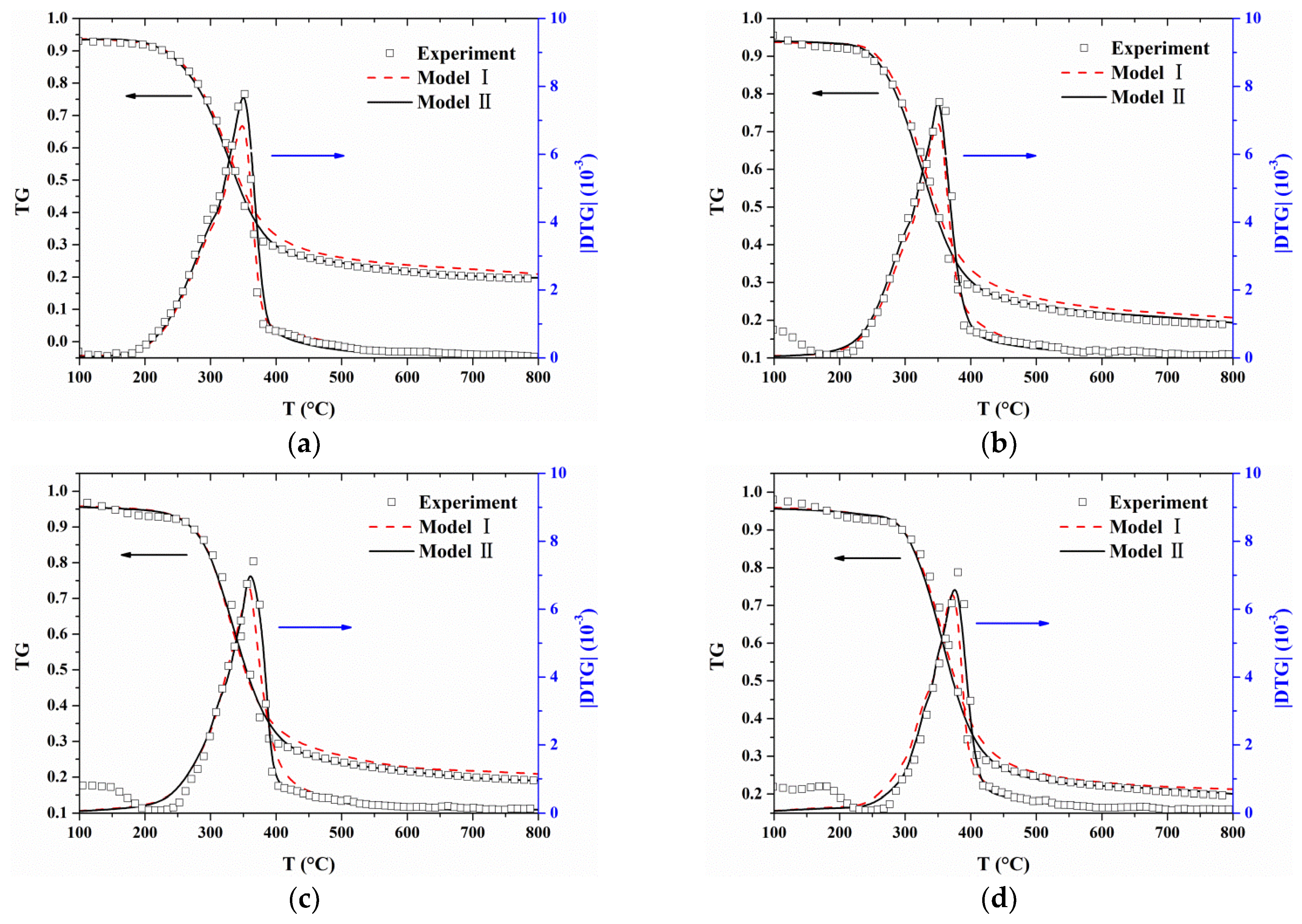
Comparisons between the experimental TG/DTG data and calculated values are presented in Figure 6. Good fitting qualities are observed at heating rates from 10 to 40 °C/min for both Model I and Model II. These optimized parameters can be found to satisfy not only the heating rates where they are calculated from (20 and 30 °C/min) but also other heating rates (10 and 40 °C/min). However, for Model I, predicted TG values are slightly larger than experimental data when the temperature is higher than 350 °C in all cases. Additionally, the peak values of the predicted |DTG| curves are smaller than the experimental data although the predicted results can capture the characteristic regions of the experimental |DTG| curves.

To further verify the reliability of the optimized parameters, the experimental curves of |DDTG| and |DTG| of MDF at 10 °C/min with the mass loss rates of four components calculated by Model I and Model II are presented in Figure 7. It can be found that the temperatures corresponding to the peak DTG of four components matches the temperatures corresponding to the four local minimum points in the |DDTG| curve. It is consistent with the conclusions drawn in Figure 3. However, the mass loss rates of four components obtained by Model I and Model II are very different.

In summary, the total TG-DTG curves calculated from both Model I and Model II fit the experimental data well, while components DTG curves obtained by models are different. Therefore, the effects of the consideration of secondary charring reactions in reaction models on components and products will be discussed in the following section.

3.4. Effects of Secondary Charring Reactions on the Components and Products

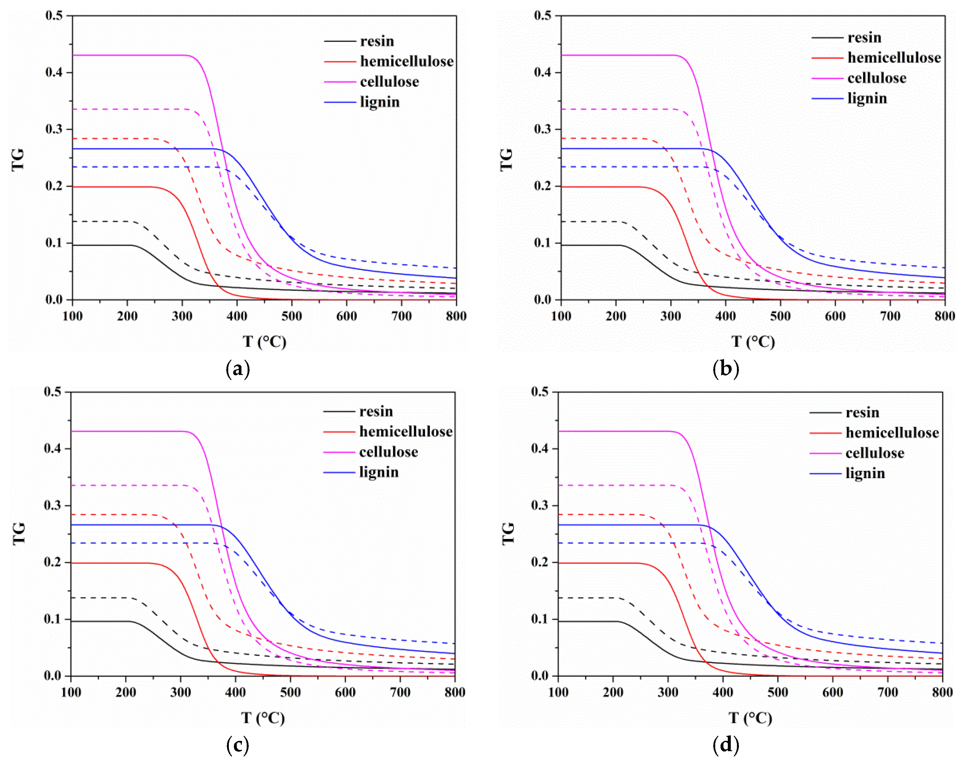
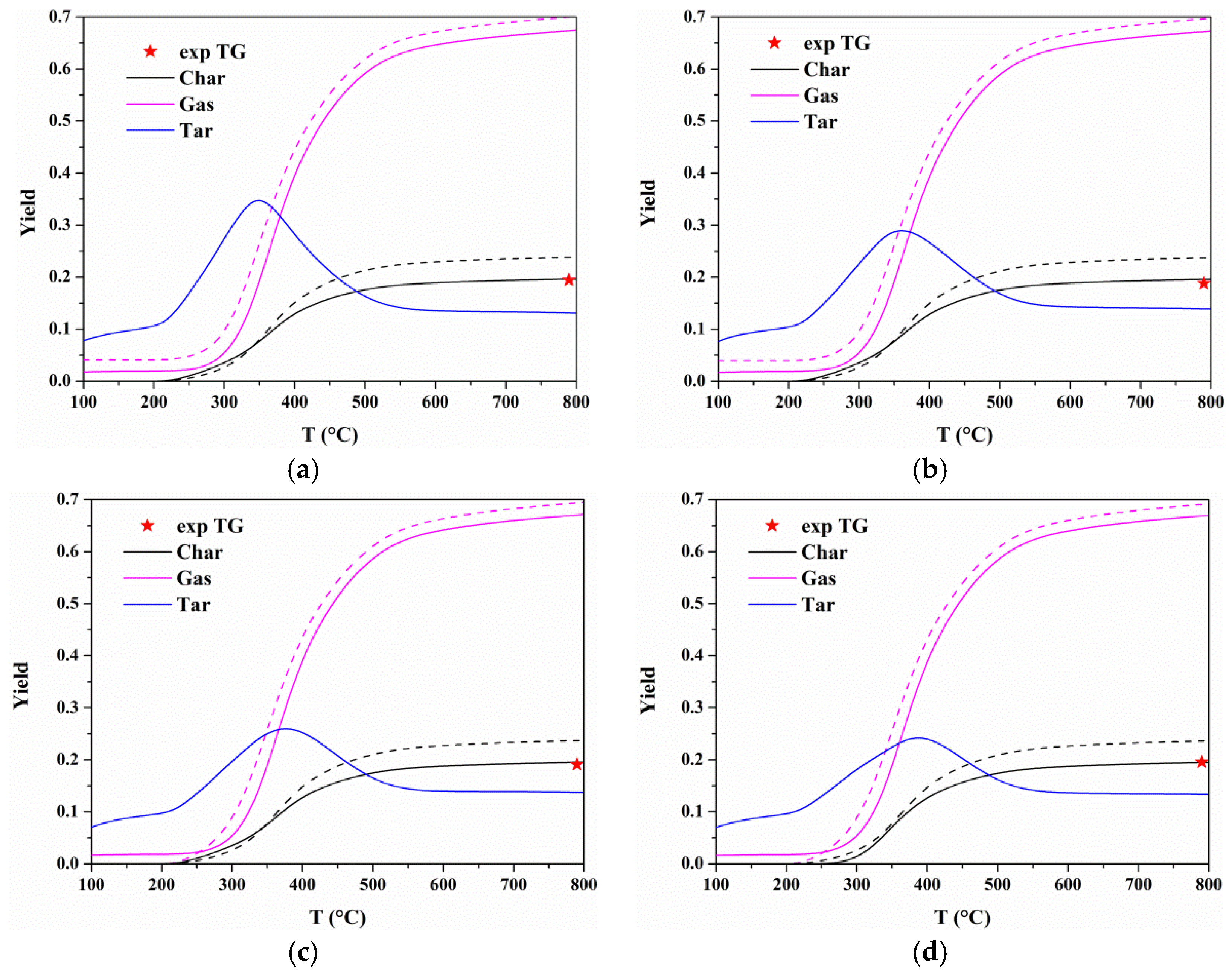
For each heating rate, the predicted TG curves of each component of the two models are plotted in Figure 8. It shows that the initial temperatures at which degradation for resin, hemicellulose, cellulose, and lignin begin are around 225, 280, 360, and 400 °C for Model I and Model II, which are consistent with the temperatures corresponding to the components peak DTG. It indicates that the secondary charring reactions have little effect on the characteristic regions of pyrolysis process. However, components contents are very different when secondary charring reactions are considered or not. Differences in components contents will affect the estimated yields of products. Figure 9 presents gas, tar, and char yields at different heating rates calculated by Model I and Model II. It shows tiny differences in the yield of each product at different heating rates for two models. In the case of 10 °C/min, the gas and char yields increase with temperature, and remain almost constant above 700 °C. Additionally, higher gas and char yields are calculated by Model I. For tar yield, it increases when T < 350 °C, and then there will be a reduction. The most possible reason is that the tar cracking which may be one of the reactions involved in secondary charring occurs at around 400 °C [23].

The char yield generated by MDF can be determined by weighing the residue amount after the experiment [45,46]. In Figure 6, the mass loss (TG) was very slow and its variation (DTG) could be ignored above 700 °C. Therefore, the solid residue amount at 800 °C was regard as the experimental char yield, which was marked by pentagram in Figure 9. Obviously, the char yield calculated by Model I is higher than experimental data. The percentage difference in the char yields between models and experiment is determined by:

$$\mathrm{Diff}.\%=\frac{\left|w_m-w_{exp}\right|}{w_{exp}}\times 100\%$$

(23)

where w_m and w_exp represent the char yield obtained from model and experiment, respectively.

Table 7. The percentage differences in the char yields between models and experiment.

Model	10 °C/min	20 °C/min	30 °C/min	40 °C/min	Mean Value
Model I	22.9%	26.6%	24.2%	20.7%	23.6%
Model II	1.1%	4.3%	2.5%	0.3%	2%

lists the percentage differences in the char yields calculated by two models. The average error of char yield for Model I in four heating rates is 23.6% while the average error is 2% for Model II. Therefore, the components’ contents and products’ yields can be better estimated by Model II.

In conclusion, it has been validated that the proposed model considering the secondary charring reactions coupled with the DE method can be applied to obtain the proper kinetic parameters. Additionally, the percentage difference in the char yields can be decreased from 23.6% to 2% when secondary charring reactions are considered.

4. Conclusions

A series of thermogravimetric experiments from 10 °C/min to 40 °C/min are performed to analyze the pyrolysis behaviors of MDF in nitrogen. The pyrolysis process of MDF can be divided into four stages corresponding to the degradation of resin, hemicellulose, cellulose, and lignin, respectively, by conversion rater α = 0.1, α = 0.2, and α = 0.8. To better describe the thermal decomposition process of MDF, a kinetic model based on multi-component parallel reaction scheme considering secondary charring reactions is proposed. Kinetic parameters are predicted by coupling the differential evolution (DE) algorithm with the proposed model. Comparison results show that the proposed model considering secondary reactions is in good agreement with experimental data at various heating rates. Moreover, with the consideration of secondary charring reactions, the error in the estimated char yield decreased from 23.6% to 2%. Therefore, the proposed model considering the secondary charring reactions is reasonable and the differential evolution is capable to find appropriate optimized kinetic parameters of biomass.

It is anticipated that our work will be helpful to describe practical thermal conversion process of biomass with more accurate predictions of kinetic parameters and products yields. Moreover, the optimized parameters can be implemented in pyrolysis or fire models in simulation tools to study more complex biomass pyrolysis and to design appropriate biomass reactors.

References

- Food and Agriculture Organization of the United Nations. Forestry Production and Trade. 2018. Available online: http://www.fao.org/faostat/en/#data/FO (accessed on 16 September 2018).
- Lubis, M.A.R.; Park, B.D.; Woo, Y.D. Characterization of recycled fibers from medium-density fiberboard for its recycling. J. Clean. Prod. 2018, 202, 456–464. [Google Scholar]
- Kabir, M.J.; Chowdhury, A.A.; Rasul, M.G. Pyrolysis of Municipal Green Waste: A Modelling, Simulation and Experimental Analysis. Energies 2015, 8, 7522–7541. [Google Scholar] [CrossRef] [Green Version]
- Bo, N.; Chen, Z.; Xu, Z. Application of pyrolysis to recycling organics from waste tantalum capacitors. J. Hazard. Mater. 2017, 335, 39–46. [Google Scholar]
- Mishra, G.; Kumar, J.; Bhaskar, T. Kinetic studies on the pyrolysis of pinewood. Bioresour. Technol. 2015, 182, 282–288. [Google Scholar] [CrossRef] [PubMed]
- Si, L.; Fan, Y.; Wang, Y.; Sun, L.; Li, B.; Xue, C.; Hou, H. Thermal degradation behavior of collagen from sea cucumber (Stichopus japonicus) using TG-FTIR analysis. Thermochim. Acta 2018, 659, 166–171. [Google Scholar] [CrossRef]
- Rong, H.; Wang, T.; Zhou, M.; Wang, H.; Hou, H.; Xue, Y. Combustion Characteristics and Slagging during Co-Combustion of Rice Husk and Sewage Sludge Blends. Energies 2017, 10, 438. [Google Scholar] [CrossRef]
- Hashim, R.; Sulaiman, O.; Kumar, R.N.; Tamyez, P.F.; Murphy, R.J.; Ali, Z. Physical and mechanical properties of flame retardant urea formaldehyde medium density fiberboard. J. Mater. Process. Technol. 2009, 209, 635–640. [Google Scholar] [CrossRef]
- Yorulmaz, S.Y.; Atimtay, A.T. Investigation of combustion kinetics of treated and untreated waste wood samples with thermogravimetric analysis. Fuel Process. Technol. 2009, 90, 939–946. [Google Scholar] [CrossRef]
- Han, T.U.; Kim, Y.M.; Watanabe, C.; Teramae, N.; Park, Y.K.; Kim, S.; Lee, Y. Analytical pyrolysis properties of waste medium-density fiberboard and particle board. J. Ind. Eng. Chem. 2015, 32, 345–352. [Google Scholar] [CrossRef]
- Shafizadeh, F.; Chin, P. Thermal deterioration of wood. ACS Symp. Ser. 1977, 43, 57–81. [Google Scholar]
- Bastiaans, R.J.M.; Toland, A.; Holten, A.; Goey, L.P.H.D. Kinetics of co release from bark and medium density fibreboard pyrolysis. Biomass Bioenergy 2010, 34, 771–779. [Google Scholar] [CrossRef]
- Koufopanos, C.A.; Maschio, G.; Lucchesi, A. Kinetic modeling of the pyrolysis of biomass and biomass components. Can. J. Chem. Eng. 1989, 67, 75–84. [Google Scholar] [CrossRef]
- Miller, R.S.; Bellan, J. A generalized biomass pyrolysis model based on superimposed cellulose, hemicellulose and lignin kinetics. Combust. Sci. Technol. 1997, 126, 97–137. [Google Scholar] [CrossRef]
- Anca-Couce, A. Reaction mechanisms and multi-scale modelling of lignocellulosic biomass pyrolysis. Prog. Energy Combust. Sci. 2016, 53, 41–79. [Google Scholar] [CrossRef]
- Manya, J.J.; Velo, E.; Puigjaner, L. Kinetics of biomass pyrolysis: A reformulated three-parallel-reactions model. Ind. Eng. Chem. Res. 2003, 42, 434–441. [Google Scholar] [CrossRef]
- Barneto, A.G.; Carmona, J.A.; Alfonso, J.E.; Serrano, R.S. Simulation of the thermogravimetry analysis of three non-wood pulps. Bioresour. Technol. 2010, 101, 3220–3229. [Google Scholar] [CrossRef] [PubMed]
- Liden, A.G.; Berruti, F.; Scott, D.S. A kinetic model for the production of liquids from the flash pyrolysis of biomass. Chem. Eng. Commun. 1988, 65, 207–221. [Google Scholar] [CrossRef]
- Li, K.Y.; Huang, X.; Fleischmann, C.; Rein, G.; Ji, J. Pyrolysis of medium-density fiberboard: Optimized search for kinetics scheme and parameters via a genetic algorithm driven by Kissinger’s method. Energy Fuels 2014, 28, 6130–6139. [Google Scholar] [CrossRef]
- White, J.E.; Catallo, W.J.; Legendre, B.L. Biomass pyrolysis kinetics: A comparative critical review with relevant agricultural residue case studies. J. Anal. Appl. Pyrol. 2011, 91, 1–33. [Google Scholar] [CrossRef]
- Neves, D.; Thunman, H.; Matos, A.; Tarelho, L.; Gomez-Barea, A. Characterization and prediction of biomass pyrolysis products. Prog. Energy Combust. Sci. 2011, 37, 611–630. [Google Scholar] [CrossRef]
- Santaniello, R.; Galgano, A.; Blasi, C.D. Coupling transport phenomena and tar cracking in the modeling of microwave-induced pyrolysis of wood. Fuel 2012, 96, 355–373. [Google Scholar] [CrossRef]
- Anca-Couce, A.; Mehrabian, R.; Scharler, R.; Obernberger, I. Kinetic scheme of biomass pyrolysis considering secondary charring reactions. Energy Convers. Manag. 2014, 87, 687–696. [Google Scholar] [CrossRef]
- Zhai, M.; Wang, X.; Zhang, Y.; Dong, P.; Qi, G.; Huang, Y. Characteristics of rice husk tar secondary thermal cracking. Energy 2015, 93, 1321–1327. [Google Scholar] [CrossRef]
- Ding, Y.; Wang, C.; Chaos, M.; Chen, R.; Lu, S. Estimation of beech pyrolysis kinetic parameters by shuffled complex evolution. Bioresour. Technol. 2016, 200, 658–665. [Google Scholar] [CrossRef] [PubMed]
- Khiari, B.; Jeguirim, M. Pyrolysis of Grape Marc from Tunisian Wine Industry: Feedstock Characterization, Thermal Degradation and Kinetic Analysis. Energies 2018, 11, 730. [Google Scholar] [CrossRef]
- Jo, J.H.; Kim, S.S.; Shim, J.W.; Lee, Y.E.; Yoo, Y.S. Pyrolysis Characteristics and Kinetics of Food Wastes. Energies 2017, 10, 1191. [Google Scholar] [CrossRef]
- Storn, R.; Price, K. Differential Evolution—A Simple and Efficient Heuristic for global Optimization over Continuous Spaces. J. Glob. Optim. 1997, 11, 341–359. [Google Scholar] [CrossRef]
- Storn, R. On the usage of differential evolution for function optimization. In 1996 Biennial Conference of the North American Fuzzy Information Processing Society-NAFIPS; IEEE Press: Piscataway, NJ, USA, 1996; pp. 519–523. ISBN 0780332261. [Google Scholar]
- Khawam, A.; Flanagan, D.R. Complementary use of model-free and modelistic methods in the analysis of solid-state kinetics. J. Phys. Chem. B 2005, 109, 10073–10080. [Google Scholar] [CrossRef] [PubMed]
- Chen, R.; Lu, S.; Zhang, Y.; Lo, S. Pyrolysis study of waste cable hose with thermogravimetry/Fourier transform infrared/mass spectrometry analysis. Energy Convers. Manag. 2017, 153, 83–92. [Google Scholar] [CrossRef]
- Doyle, C.D. Estimating isothermal life from thermogravimetric data. J. Appl. Polym. Sci. 1962, 6, 639–642. [Google Scholar] [CrossRef]
- Starink, M.J. Activation energy determination for linear heating experiments: Deviations due to neglecting the low temperature end of the temperature integral. J. Mater. Sci. 2007, 42, 483–489. [Google Scholar] [CrossRef]
- Starink, M. The determination of activation energy from linear heating rate experiments: A comparison of the accuracy of isoconversion methods. Thermochim. Acta 2003, 404, 163–176. [Google Scholar] [CrossRef]
- Martín-Lara, M.A.; Blázquez, G.; Zamora, M.C.; Calero, M. Kinetic modelling of torrefaction of olive tree pruning. Appl. Therm. Eng. 2017, 113, 1410–1418. [Google Scholar] [CrossRef]
- Ferreira, S.D.; Altafini, C.R.; Perondi, D.; Godinho, M. Pyrolysis of Medium Density Fiberboard (MDF) wastes in a screw reactor. Energy Convers. Manag. 2015, 92, 223–233. [Google Scholar] [CrossRef]
- Amutio, M.; Lopez, G.; Alvarez, J.; Moreira, R.; Duarte, G.; Nunes, J.; Olazar, M.; Bilbao, J. Pyrolysis kinetics of forestry residues from the Portuguese Central Inland Region. Chem. Eng. Res. Des. 2013, 91, 2682–2690. [Google Scholar] [CrossRef]
- Kercher, A.K.; Nagle, D.C. TGA modeling of the thermal decomposition of CCA treated lumber waste. Wood Sci. Technol. 2001, 35, 325–341. [Google Scholar] [CrossRef]
- Xu, L.; Jiang, Y.; Wang, L. Thermal decomposition of rape straw: Pyrolysis modeling and kinetic study via particle swarm optimization. Energy Convers. Manag. 2017, 146, 124–133. [Google Scholar] [CrossRef]
- Ma, Z.Q.; Chen, D.Y.; Gu, J.; Bao, B.F.; Zhang, Q.S. Determination of pyrolysis characteristics and kinetics of palm kernel shell using TGA-FTIR and model-free integral methods. Energy Convers. Manag. 2015, 89, 251–259. [Google Scholar] [CrossRef]
- Chen, X.; Liu, L.; Zhang, L.; Zhao, Y.; Zhang, Z.; Xie, X.; Qiu, P.; Chen, G.; Pei, J. Thermogravimetric analysis and kinetics of the co-pyrolysis of coal blends with corn stalks. Thermochim. Acta 2018, 659, 59–65. [Google Scholar] [CrossRef]
- Yao, Z.; Ma, X.; Wu, Z.; Yao, T. TGA–FTIR analysis of co-pyrolysis characteristics of hydrochar and paper sludge. J. Anal. Appl. Pyrol. 2017, 123, 40–48. [Google Scholar] [CrossRef]
- Wang, G.; Zhang, J.; Shao, J.; Ren, S. Characterisation and model fitting kinetic analysis of coal/biomass co-combustion. Thermochim. Acta 2014, 591, 68–74. [Google Scholar] [CrossRef]
- Munir, S.; Daood, S.; Nimmo, W.; Cunliffe, A.; Gibbs, B. Thermal analysis and devolatilization kinetics of cotton stalk, sugar cane bagasse and shea meal under nitrogen and air atmospheres. Bioresour. Technol. 2009, 100, 1413–1418. [Google Scholar] [CrossRef] [PubMed]
- Hao, Q.L.; Bo-Lun, L.I.; Liu, L.; Zhang, Z.B.; Dou, B.J.; Wang, C. Effect of potassium on pyrolysis of rice husk and its components. J. Fuel Chem. Technol. 2015, 43, 34–41. [Google Scholar] [CrossRef]
- Trendewicz, A.; Evans, R.; Dutta, A.; Sykes, R.; Carpenter, D.; Braun, R. Evaluating the effect of potassium on cellulose pyrolysis reaction kinetics. Biomass Bioenergy 2015, 74, 15–25. [Google Scholar] [CrossRef] [Green Version]
Figure 1.
Multi-component competitive scheme of biomass pyrolysis including secondary charring.
Figure 2.
Curves of MDF at different heating rates: (a) TG; and (b) |DTG|.
Figure 3.
Corresponding curves of MDF at 10 °C/min: (a) |DDTG|; and (b) |DTG|.
Figure 4.
(a) FWO plots; (b) KAS plots; (c) Starink plots at the conversion of 0.1–0.9; and (d) activation energy E and temperature at 10 °C/min versus conversion α.
Figure 5.
lnA versus E using FWO and the third order reaction model at 0.2 < α ≤ 0.8.
Figure 6.
Comparisons between experimental TG/DTG data and predictions based on optimized parameters: (a) β = 10 °C/min; (b) β = 20 °C/min; (c) β = 30 °C/min; and (d) β = 40 °C/min.
Figure 7.
Experimental curves of |DDTG| and |DTG| of MDF at 10 °C/min with four components by: Model I is shown in dashed lines; Model II is shown in solid lines.
Figure 8.
Comparisons of components mass between Model I and Model II at four heating rates: (a) 10 °C/min; (b) 20 °C/min; (c) 30 °C/min; and (d) 40 °C/min. Model I is shown in dashed lines, and Model II is shown in solid lines.
Figure 9.
Comparisons of product yields between Model I and Model II at four heating rates: (a) 10 °C/min; (b) 20 °C/min; (c) 30 °C/min; and (d) 40 °C/min. Model I is shown in dashed lines, and Model II is shown in solid lines.