Article

Implementation Strategy of Convolution Neural Networks on Field Programmable Gate Arrays for Appliance Classification Using the Voltage and Current (V-I) Trajectory

by
Darío Baptista
1,2,3,*,
Sheikh Shanawaz Mostafa
1,2,
Lucas Pereira
2,
Leonel Sousa
1,3 and
Fernando Morgado-Dias
2,4
1
Instituto Superior Tecnico, Universidade de Lisboa, 1649-001 Lisbon, Portugal
2
M-ITI—Madeira Interactive Technologies Institute, 9020-105 Funchal, Portugal
3
INESC-ID Instituto de Engenharia de Sistemas e Computadores—Investigação e Desenvolvimento, DEEC, 1000-029 Lisbon, Portugal
4
Ciências Exatas e Engenharia, UMa-University of Madeira, 9020-105 Funchal, Portugal
*
Author to whom correspondence should be addressed.
Energies 2018, 11(9), 2460; https://doi.org/10.3390/en11092460
Submission received: 26 July 2018 / Revised: 8 September 2018 / Accepted: 10 September 2018 / Published: 17 September 2018
(This article belongs to the Special Issue 10 Years Energies - Horizon 2028)

Abstract

:
Specific information about types of appliances and their use in a specific time window could help determining in details the electrical energy consumption information. However, conventional main power meters fail to provide any specific information. One of the best ways to solve these problems is through non-intrusive load monitoring, which is cheaper and easier to implement than other methods. However, developing a classifier for deducing what kind of appliances are used at home is a difficult assignment, because the system should identify the appliance as fast as possible with a higher degree of certainty. To achieve all these requirements, a convolution neural network implemented on hardware was used to identify the appliance through the voltage and current (V-I) trajectory. For the implementation on hardware, a field programmable gate array (FPGA) was used to exploit processing parallelism in order to achieve optimal performance. To validate the design, a publicly available Plug Load Appliance Identification Dataset (PLAID), constituted by 11 different appliances, has been used. The overall average F-score achieved using this classifier is 78.16% for the PLAID 1 dataset. The convolution neural network implemented on hardware has a processing time of approximately 5.7 ms and a power consumption of 1.868 W.

1. Introduction

Non-intrusive load monitoring (NILM), is an energy analytics discipline that hinging on machine-learning and signal-processing techniques estimates the consumption of individual appliances from global measurements taken at a limited quantity of locations in the grid [1]. NILM has gained prominence due to the potential of using individual appliance consumption to promote energy saving behavior in individuals and to power a number of applications in support of the energy efficient home concept, which are expected to significantly reduce the carbon footprint associated with electric energy consumption [2].
Throughout the years, a great number of algorithms have been proposed to solve the problem of energy disaggregation [3,4]. These algorithms are categorized into either event-based or event-less, based on the disaggregation approach [5].
Event-based approaches seek to disaggregate the total consumption by detecting and classifying as much individual appliance transitions as possible (also known as power events). These approaches are mostly supervised, and rely on previously trained event detection, classification and energy estimation algorithms. On the other hand, event-less algorithms seek to disaggregate the signal sample-by-sample, by assigning each sample of the aggregated power consumption to the total consumption of a specific combination of appliances. Approaches under this category are mostly unsupervised or semi-supervised by means of statistical and probabilistic algorithms. This paper focuses on event-based approaches.
A key component of event-based approaches is the process of classifying samples, using features extracted from the vicinity of the power changes. From a high-level perspective, such features are classified as belonging to one of two categories: (i) engineered, and (ii) data-driven [6]. The former category contains features defined based on the domain knowledge about the discriminatory patterns of individual appliances, whereas the latter refers to features that are learned automatically from the data without any prior input (i.e., unsupervised feature learning).
In the most recent years, 2-dimensional voltage-current (V-I) trajectories [7] have received special attention from the community as a way of characterizing load signatures in terms of features in the two categories referred above. The V-I trajectories are obtained by plotting the normalized steady-state voltage and current signals corresponding to one-cycle, sampled at high-frequencies (≥1 kHz). A basic assumption considers that for appliances with different working principles (e.g., resistive or inductive), the corresponding V-I trajectory exhibits unique characteristics that can be captured by wave-shape (WS) features [7,8]. Engineered features are extracted directly from the WS, and include the looping direction, the enclosed area and the number of self-intersections [7,8]. On the other hand, data driven features are mainly extracted by treating the V-I shape as binary images and applying dimensionality reduction techniques like principal component analysis (PCA) [6] or deep-learning techniques like convolutional neural networks (CNN) [9].
While this is a very promising approach to the disaggregation problem (see Section 2), the downside of using V-I trajectories is the high-computational burden required to extract the trajectories and the current features, which unfortunately cannot be met by traditional smart-meters. Therefore, the processing of such system is mostly deferred to the cloud which implies high-bandwidth long duration communications to send the high-frequency current and voltage waveforms, contrasting the recent trend in internet of thing (IoT) communications that favors high-throughput of small packages across large distances. On the other hand, this implies that near-real time disaggregation would no longer be possible, which is crucial for some NILM applications, such as grid quality diagnostics.
Therefore, an alternative would be to compute locally, part or the whole processing, using hardware implementations, for example through field programming gate arrays (FPGAs) or application-specific integrated circuits (ASICs). Ultimately, a hardware implementation would mean that all the heavy processing would be performed locally, hence avoiding the communication overheads, since only the actual appliance classification would have to be communicated. Furthermore, the high-speed enabled by hardware implementations would enable close to real-time disaggregation, which would otherwise be hard to achieve.
Likewise, another aspect where hardware implementations can be advantageous, is related to the privacy issues raised by the potential of energy consumption data to reveal sensitive information such as home occupation patterns, and the number of occupants [10]. This topic has raised the attention of a number of researchers, who have proposed different solutions to protect the end-users from such risks by making it harder to access and/or interpret the energy consumption data. The proposed solutions include masking the load variations using in-house battery energy storage systems (BESS) [11], or adding noise to the load signals [12,13]. Still, while this guarantees the privacy of the end-users, it makes the disaggregation problem and any other kind of inference much harder, which may not be desirable from the utility point of view [13]. As such, solutions based on homomorphic encryption were proposed as a mean to allow the application of disaggregation and other inference techniques on top of the encrypted data. Still, solutions-based homomorphic encryption comes at the expense of huge computational costs, and the need to hire third-party agents for key distribution and management [13].
In our particular case, since all the computation is done locally and only the disaggregation results need to be made available to the cloud, much simpler encryption techniques can be used to protect the communication channel.
A hardware implementation of a NILM system based on V-I curves (Section 2.1) and a CNN (Section 2.2) is proposed in this paper. More concretely, the research contributions of this work are two-fold: a new deep-learning approach for classification in NILM was developed and a hardware architecture to efficiently run the trained CNN on FPGA (Section 3.4) was implemented. The proposed algorithm and architecture were used for designing the hardware system. They are both evaluated (results are shown in Section 4) using the Plug Load Appliance Identification Dataset (PLAID) (Section 3.1) with different performance parameters (Section 3.5).

2. Background and Related Work

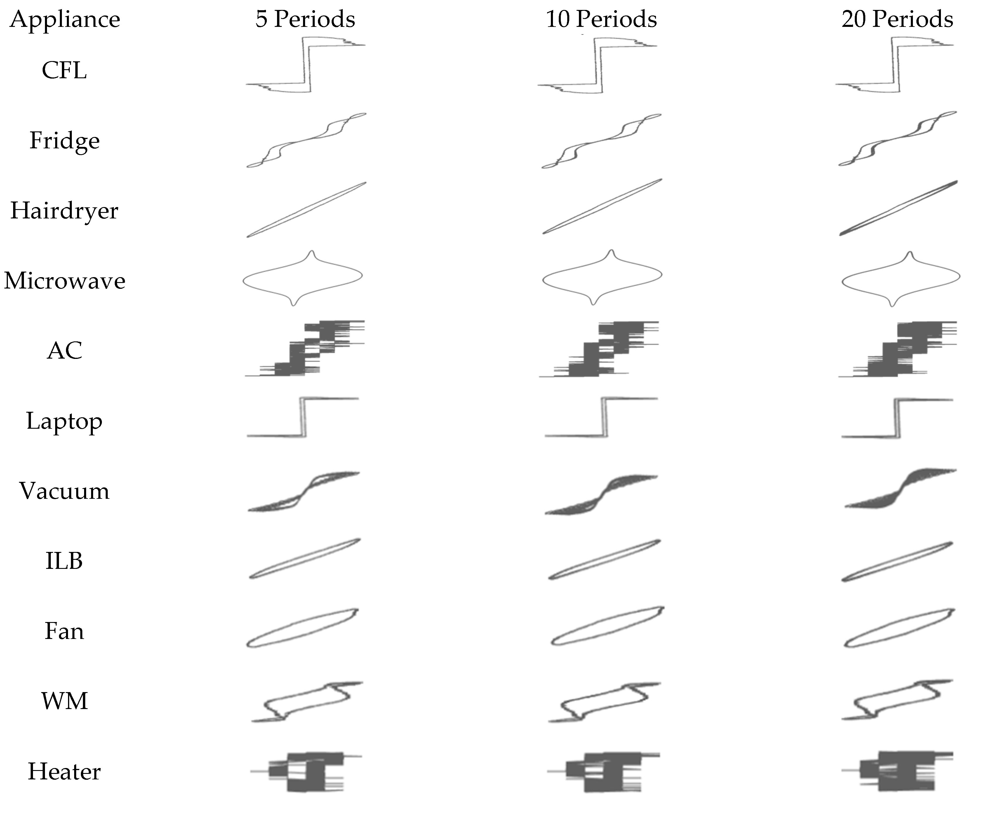
2.1. V-I Shapes and NILM

V-I shapes were first applied to NILM research by Lam et al. [7]. It was shown that WS features based on the V-I trajectories provide high discrimination among different types of appliances. Later, Hassan et al. [8], extended the original set of WS features, and performed an empirical validation of such features using the REDD dataset [14]. More concretely, they benchmarked the WS features against standard features (real and reactive power consumption—PQ, and the harmonic content of the current waveforms—HAR) using four benchmark algorithms (artificial neural networks—ANN, artificial neural network coupled with an evolutionary algorithm—ANN-EA, support vector machines—SVM, and adaptive boosting—AdaBoost). Ultimately, the obtained results have shown that the selected WS outperform the traditional features in all four problems, further suggesting the high-discrimination capability of such features. Iksan et al. [15] have evaluated the potential of including two WS features (enclosed area—EA, and curvature of the mean line—CML) in a hybrid signature along with active power—P, reactive power—Q, power factor—PF, and total harmonic distortion—THD. Their approach was tested against the REDD dataset using a Naïve Bayes algorithm, and the results have shown an increase from 55% to 91% in the overall classification accuracy when EA and CML were added to the feature space.
To the best of our knowledge, the first approach to extract data-driven features from V-I shapes was the work of Gao et al. [6] using the PLAID dataset [16]. This work has converted the normalized V-I shapes to binary images for training machine-learning (k-nearest neighbor (1-NN), logistic regression classifier—LGC, Gaussian naïve Bayes—GNB, SVM, decision trees—DT, and random forests—RF). In this setup, the best average accuracy was obtained for the raw binary image with 81.75%, whereas the principal components achieved an average accuracy of 77.65%. Nevertheless, the best accuracy (86.03%) was obtained when combining the raw binary image with engineered features (P, Q, the first 11 odd harmonics, and the quantized version of the current waveform). In [17] the authors expanded the work from [6] and the raw steady-state current and voltage waveforms as training data for an ensemble of neural networks. Their approach was also tested against PLAID, and the obtained results show an average accuracy of 89%. In order to improve the discriminative power of V-I trajectories within appliance categories, Du et al. [18] have proposed novel methods to create binary images from V-I trajectories and to extract learning features from such images (e.g., the number of continuums of occupied cells , and the existence or not of self-interceptions). The proposed methods were extensively tested against an undisclosed dataset using a supervised self-organizing map (SSOM) learning algorithm. The obtained results showed an average accuracy of 99%.
Strategies from object recognition were also attempted in [19]. Contours and elliptical Fourier descriptors were combined to extract features from the binary representation of the V-I trajectories. The proposed features were evaluated against the PLAID dataset using three supervised learning algorithms (ANN, logistic regression—LR, and RF). The results have shown an average accuracy of about 80% for the RF, which is comparable to those reported in [6] but still far from the results shown in [17] for the same dataset.
Finally, De Beaets et al. [9] proposed an application of CNNs to discriminate among weighted pixelated image representations of the V-I trajectories. The proposed approach was tested against two datasets, PLAID [16] and WHITED [20]. The obtained results were reported using the F-measure for individual appliance classification, and the macro-average F-measure for the overall classification. The reported macro F-measures were 77.6% and 75.46% for PLAID and WHITED, respectively.

2.2. Convolution Neural Network Backgroud

Because of the distinguishable signature in the V-I trajectory picture, visual deep learning has been used to classify different appliances. One of the most popular types of visual deep learning classifier to processing 2D data is known as CNN [21]. A CNN extracts local features at high resolution and combines them into high-level complex features at low resolutions. In order to achieve this goal, CNNs have convolution and pooling layers accompanied with activation functions and, in the end, there are a fully connected layer with a softmax function [22]. The convolution layer produces at the output a feature map using different convolution kernels [23]. During the training phase, the CNN learns the values of the kernels for a particular task [24]. Taking into account the entire convolution layer, the feature maps can be seen as a three-dimensional (3D) map [25]. The equation for the feature map of the 3D convolution layer is given by Equation (1).
  C d = φ ( k d f + b d )  
where   1 d < n k d ,   n k d is the number of convolution kernels in a layer, C is the feature map of the entire convolution layer ( C i × j × n k d ), is the 2D convolution operation, k is the kernel, f is the input matrix, b is the bias and φ is the rectified linear unit (ReLU) given by Equation (2).
  φ ( x ) = { 0 ,   x < 0 x ,   x 0  
The other layer of the CNN is the pooling layer, with nonlinear activation functions. It down-samples feature maps of the previous layer, reducing the artifacts and sharp variations on the signal that comes out from the convolution layer [26]. In the pooling layer, the max-pooling ( σ p o o l ) is applied followed by the ReLU function [25]. The pooling layer output (P) can be expressed by Equation (3).
  P d = φ ( σ p o o l ( f d ) )  
f represents the intermediate feature maps and d is the number of pooling filters in the layer.
The fully-connected layer, whose basic element is a neuron, is the last layer in the CNN. A neuron is based on a simple function defined by Equation (4) [27].
Y = φ ( j = 1 n   f j × w j + b )  
where f is the input, w the weight, n the number of inputs and φ is the softmax function. Also known by normalized exponential function [28] , can be used to represent a categorical distribution, that is, a probability distribution over k different possible outcomes (Equation (5)).
P ( y = j | x ( i ) ) = φ s o f t m a x ( x ( i ) ) = e x ( i ) j = 0 k e x k ( i )  

2.3. FPGA Implementations of NILM and CNNs

For mitigating the individual load management problem, several attempts to deploying hardware and software platforms have been made. For example, using a multi-channel data acquisition board (LabJack U6) with a processing unit (Toshiba NB300, Tokyo, Japan) [29]. However, this implementation has two-fold limitations. First, a full mini laptop (Toshiba NB300) was connected with the sensor (LabJack U61) and, then, the appliance identification is made on-line. By using on-line identification method, the system has to transfer a lot of raw data producing a huge amount of data to be communicated through the internet. For that reason, this kind of system could not operate in low bandwidth connections. In addition to this, [30,31] are other works aimed primarily at increasing the processing speed of the underlying NILM systems using FPGAs. Remscrim et al. [30] propose the implementation of a spectral envelope processor consisting of four subsystems to: (i) current and voltage acquisition; (ii) compute the spectral envelope coefficients; (iii) store the computed coefficients on an erasable memory, and (iv) transmit the coefficients via Wi-Fi. Trung et al. [31] propose to use an FPGA to implement a cumulative-sum (CUMSUM) filter for real-time noise reduction in commercial and industrial installations. Note that in any of those cases, the actual classification step is not performed on the FPGA itself.
In the present work, a Zynq System-on-a-Chip (SoC) was used to implement a CNN classifier for identifying appliances. This SoC has a dual-core ARM Cortex-A9 processors and an FPGA (28 nm Artix-7 based). An important aspect of this implementation is the possibility of connecting to data acquisition sub-system and internet through the processor. The main contribution of this work is the execution of a CNN for appliance identification on an FPGA. The advantage of using FPGA is the exploration of parallelism to speed up the process. Figure 1 depicts the proposed system using a Zynq device.
The implemented CNN is connected to the Processing Subsystem (PS) to ensure a correct communication with the ARM CPU. This connection was made through a direct memory access (DMA), in the programmable logic (PL) subsystem. The DMA is connected through an extended interface to move data into and from the design—exploiting the Advanced eXtensible (AXI) handshake protocol [32].
A specific computational engine is an efficient requisite to implement a CNN on the FPGA. One of the first CNN implementations on hardware dates back to the early 90’s where an ANNA chip (a mixed analog/digital neural-network chip) was used to implement a CNN [33,34,35]. Korekado et al. [36] proposed a VLSI architecture of high performance and low power was used to implement a CNN. This architecture uses a hybrid approach composed of pulse-width modulation (PWM) and a digital circuitry. Fieres et al. [37] combined digital multiple FPGA-VLSI mixed models are combined to implement the first model simulated on computer by Fukushima et al. [21]. Farabet et al. [38] propose a different implementation of a CNN on an FPGA. In this implementation, all basic operations of a CNN were implemented at hardware level (e.g., 2D convolution; 2D pooling; etc.) and macro-instructions are provided to execute them in any order. The sequencing of operations is managed at software level based on a PowerPC processor (e.g., management of data transfer from/to an external system; store/retrieve kernels from/to external memory).
More recently, CNN accelerators designed based on high level synthesis (HLS) approaches have been developed. Zhang et al. [39] shows an optimized CNN accelerator designed with HLS, reordering and tiling loops, inserting pragmas and organizing external memory transfers. In [40] CNNs were implemented on HLS by adopting an N-fold approach, particularly suitable for devices with strict restrictions on power and resources consumption. Cost-effective acceleration of CNNs on FPGAs at datacenter scale has been studied by Ovtcharov [41].
CNNs have been widely adopted in many applications, either using Graphics Processing Unit (GPU) or dedicated hardware [40,41,42]. Contrariwise to V-I shapes, and the disaggregation problem overall that have received a great amount of attention from the research community in the past few years, the use of CNN as appliance identifiers, mainly on FPGA implementation, are very scare in the NILM domain.

3. Materials and Methods

3.1. Dataset

The Plug Load Appliance Identification Dataset (PLAID) [16] is used in this work. The dataset actually contains two datasets: PLAID 1 has 1074 samples and PLAID 2 has 719 samples, for a total of 1793 samples. PLAID 2 has been released recently (in 2017). Most of literature using the PLAID dataset refers to the PLAID 1 dataset. PLAID 1 was obtained from 55 houses and PLAID 2 was obtained from nine houses. Both datasets were combined for training the deep neural network. Thus, the data was created by combining PLAID 1 and PLAID 2 dataset resulting in a total of 64 houses. This dataset, collected in Pittsburgh (PA, USA), is constituted by current values and voltage values measured from 11 different electrical appliances—compact fluorescent lamp (CFL), fridge, hairdryer, microwave, air conditioner (AC), laptop, vacuum, fan, washing machine (WM), incandescent light bulb (ILB) and heater—in more than 60 houses. The sampling frequency is 30 kHz. The system was tested using leave one house out method. The sample is done without replacement.

3.2. Data Pre-Processing

A voltage and current trajectory (V-I) was mapped on a 2D plot, producing a disguisable signature or pattern for each appliance [7,8]. This plot can be used for classification of different appliances by using visual feature of the plot or picture such as shape. Voltage   ( v ) and current   ( i ) were acquired over time at a sampling frequency ( f s ) and grid frequency   (   f g ) . Once the complete period, the resultant wave is described by Equation (6) [17].
  φ p = [ φ ( p ) ,   φ ( p + 1 ) , , φ ( p + d 1 ) ] T ϵ d ,   φ ϵ { i , v }  
where d is the number of samples per period ( f s / f g ) and p   is a point in time. When more than one period of φ p   is collected, the resultant wave is named window size. In this work, three different window sizes were analyzed: 83 ms (5 periods), 166 ms (10 periods) and 333 ms (20 periods). Figure 2 shows the graphical representation of the V-I trajectory for each appliance and window size.
Visualizing the individual signature requires that data is summarized and sampled in such a way that represents the number of points that are plotted on the screen. Although each appliance presents its individual signature [8], different brands or models could present signatures with different magnitudes due to their different power consumption [7]. Because of this, getframe function from Matlab2018 was used keeping the same size in the axes as the maximum and minimum of the periods was used. Lastly, imresize function from Matlab2018 was used to reduce images to 50 × 50 dimension.

3.3. CNN for Appliance Classification

The input of the network is a 50 × 50 matrix which is considered as a single channel image. The first layer, C1, performs four convolutions with 3 × 3 kernels on the input, producing 4 feature maps of size 48 × 48. In the second layer, P1, executes 2 × 2 spatial pooling of each feature map. The third layer, C2, performs 3 × 3 convolutions to calculate high-level features. Layer P2 performs 2 × 2 pooling similar to P1. The C3 layer performs 3 × 3 convolutions. Finally, F1 is a linear classifier having 11 neurons containing the softmax function as activation function. The CNN architecture is summarized in Table 1.
The Adam algorithm with a learning rate of 0.001 was used to compute the trainable parameters using Adam algorithm along of 200 epochs, which is justifiable by the large data set used [43].

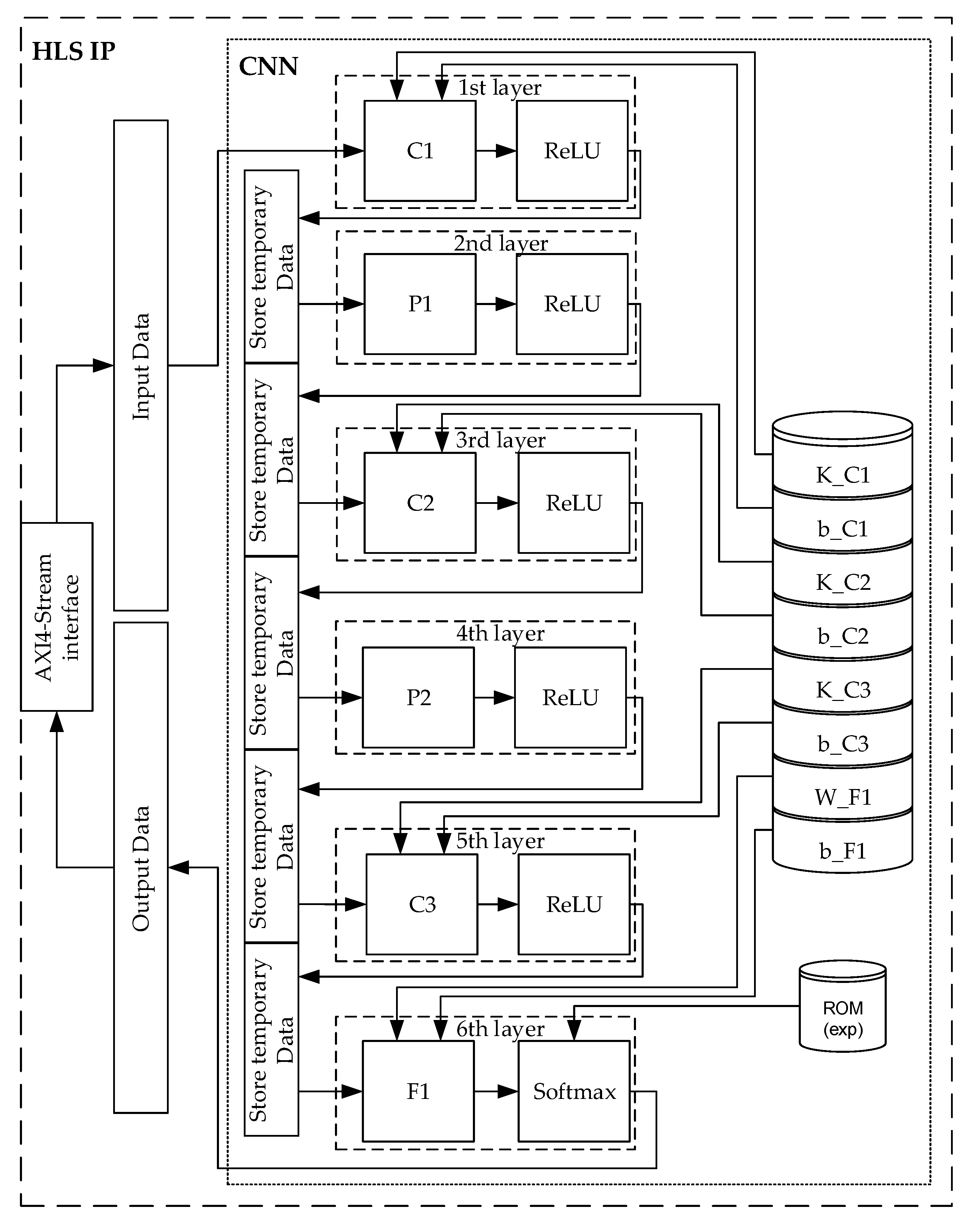
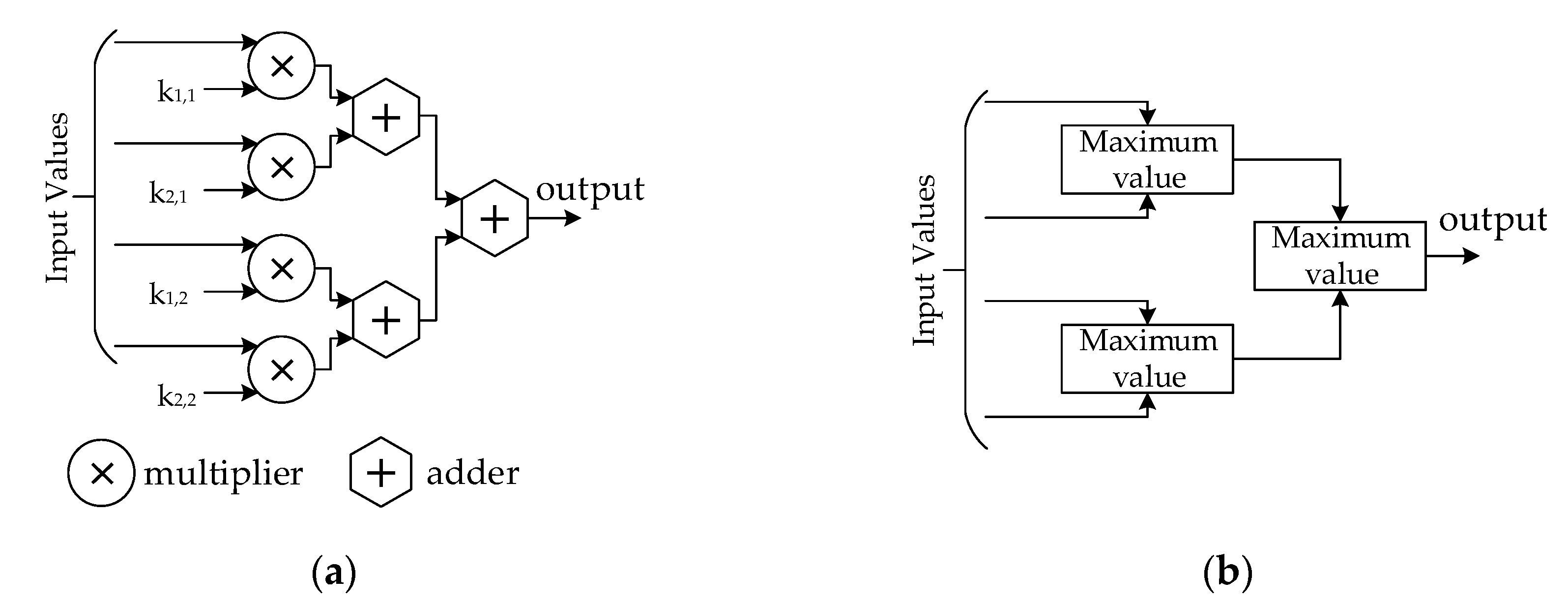
3.4. CNN Implementation on FPGA

The CNN described in the previous section (Table 1) was modeled in C code. Through of a Register Transfer Level (RTL) design, the solution was optimized and exported as an intellectual property (IP) core. Therefore, the IP was implemented on a FPGA. FPGAs use hardware for configurable processing logic (PL), thus making these very fast and flexible processing devices. Figure 3 depicts the proposed CNN architecture implemented on the IP core.
In the first part, the design computes the respective operating layer, i.e., convolution—C, pooling—P or full—F operation. The kernel—K, bias—b and weight—W values are accessed from memory to execute the convolution and full operation, respectively. Also, loop unrolling was applied to exploit parallelism between loop iterations. It creates multiple copies of the loop body. More parallelism means higher system performance and, consequently, more throughput. The objective of optimization is to enable efficient loop unrolling for fully using all the resources provided by the FPGA. Taking into account the resources available in 28 nm Artix-7 [44], adopted in this work, there were available resources to implement the parallelism in the multiplication/accumulation for the convolution (Figure 4a) and filter pooling (Figure 4b).
In the second part of the CNN design, shown in Figure 3, the activation function is computed (ReLU or softmax function). The approach to compute the ReLU considers for the domain x0 then f(x) = 0 otherwise, f(x) = x.
The implementation of the softmax function on a FPGA is itself a very challenging task. A hybrid solution was implemented on hardware to compute the exponential function. The hybrid solution consists in decomposing the exponent function into an integer and a fractional part (Equation (7)).
  e x = e i n t ( x ) × e f r a c ( x )  
where frac(x) represents the fractional part of x and int(x) is the integer part of x. The e f r a c ( x ) values are calculated through a polynomial interpolator. Chebyshev interpolation, with the interpolation nodes more concentrated in the extremity comparatively to the classic techniques, was adopted [45,46]. The e i n t ( x ) values are stored in a ROM [47], in this implementation values between e−30 to e30 are stored.
Lastly, the design implemented on hardware was exported as an IP core and its integration into a functional FPGA design was completed using the software Vivado Design Suite (Xilinx, San Jose, CA, USA).

3.5. Evaluation Metrics

The F-Score is used to measure the classification performance in order to compare this classifier with previous publications already referred. The F-Score is the balance between of precision and sensitivity for each appliance. Per appliance of each house, F-Score can be expressed as:
  F m = 2 × P P V × T P R P P V + T P R  
  p r e c i s i o n m = P P V m = T P m T P m + F P m  
  s e n s i t i v i t y m = T P R m = T P m T P m + F N m  
where m representing the m-th house, T P m representing the true positives (i.e., the quantity of appliance appropriately labeled as belonging to the positive class), F P m is the false positives (i.e., the quantity of appliance erroneously labeled as belonging to the class) and F N m is the false negatives (i.e., the quantity of appliance which were not labeled as belonging to the positive class but should have been). Lastly, the average of all the F-measures are calculated using Equation (11).
  F k = 1 M m = 1 M F m  

3.6. Power and Temperature Effects on the FPGA

On the other hand, in the implementation on FPGA, the total on-chip power on the FPGA is the power consumed inside the FPGA. The thermal power is given by Equation (12) [48,49].
  P = P d y n a m i c + P s t a t i c  
The dynamic power depends on the activity and capacitance of the circuit, while the static power depends on the process properties, manufacturing, the device junction temperature and applied voltage. The device junction temperature is the temperature of the device operation (Equation (13)) [48,49].
  T J A = T A + P θ J A  
where T A is the temperature of the environment, θ J A is the effective thermal resistance, which describes the quantity of power is dissipated from the FPGA silicon to the environment. The maximum junction temperature supported by the Zynq 7000 device (Xilinx, San Jose, CA, USA) is 85 °C [50].

4. Results and Discussion

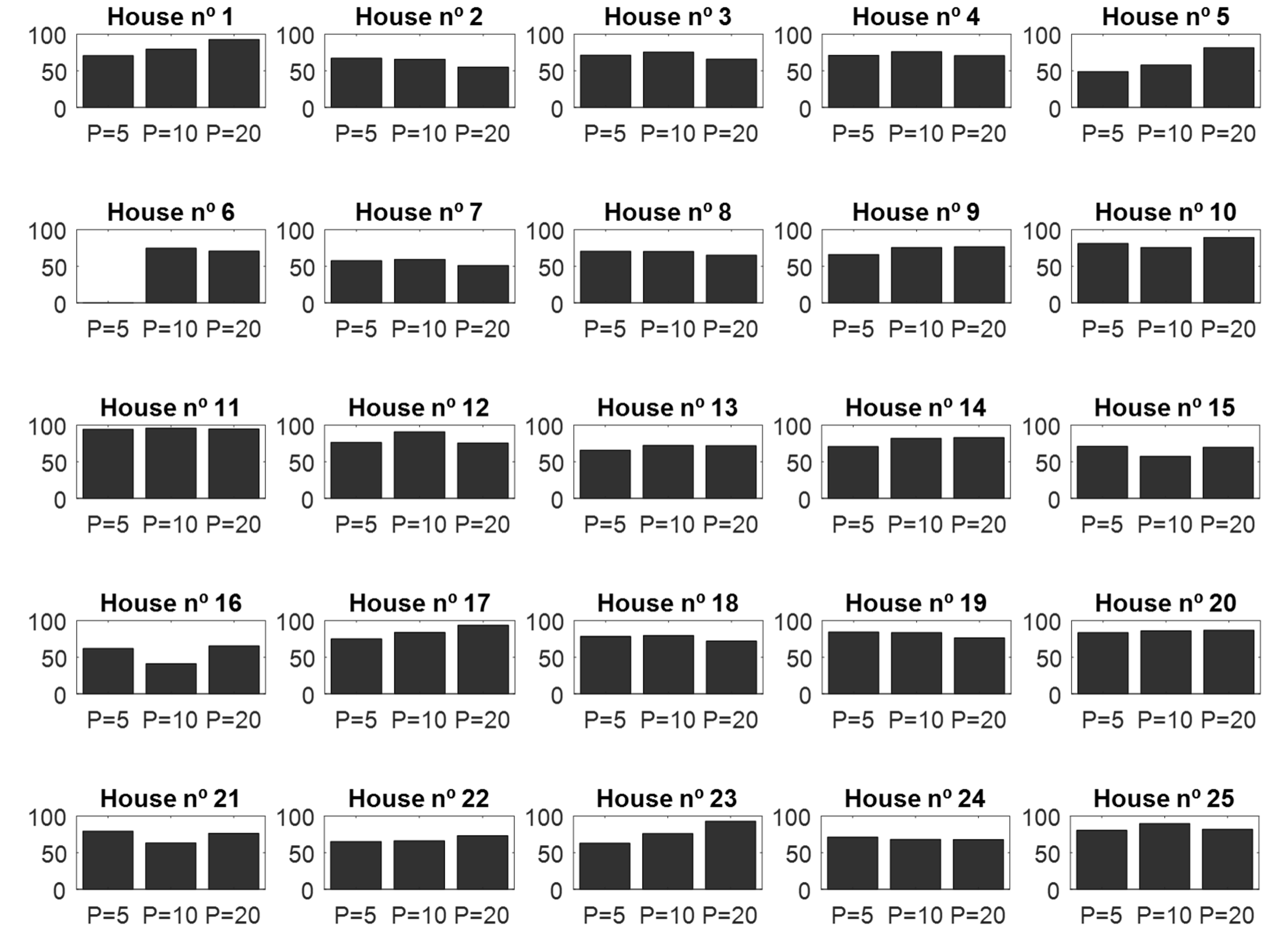
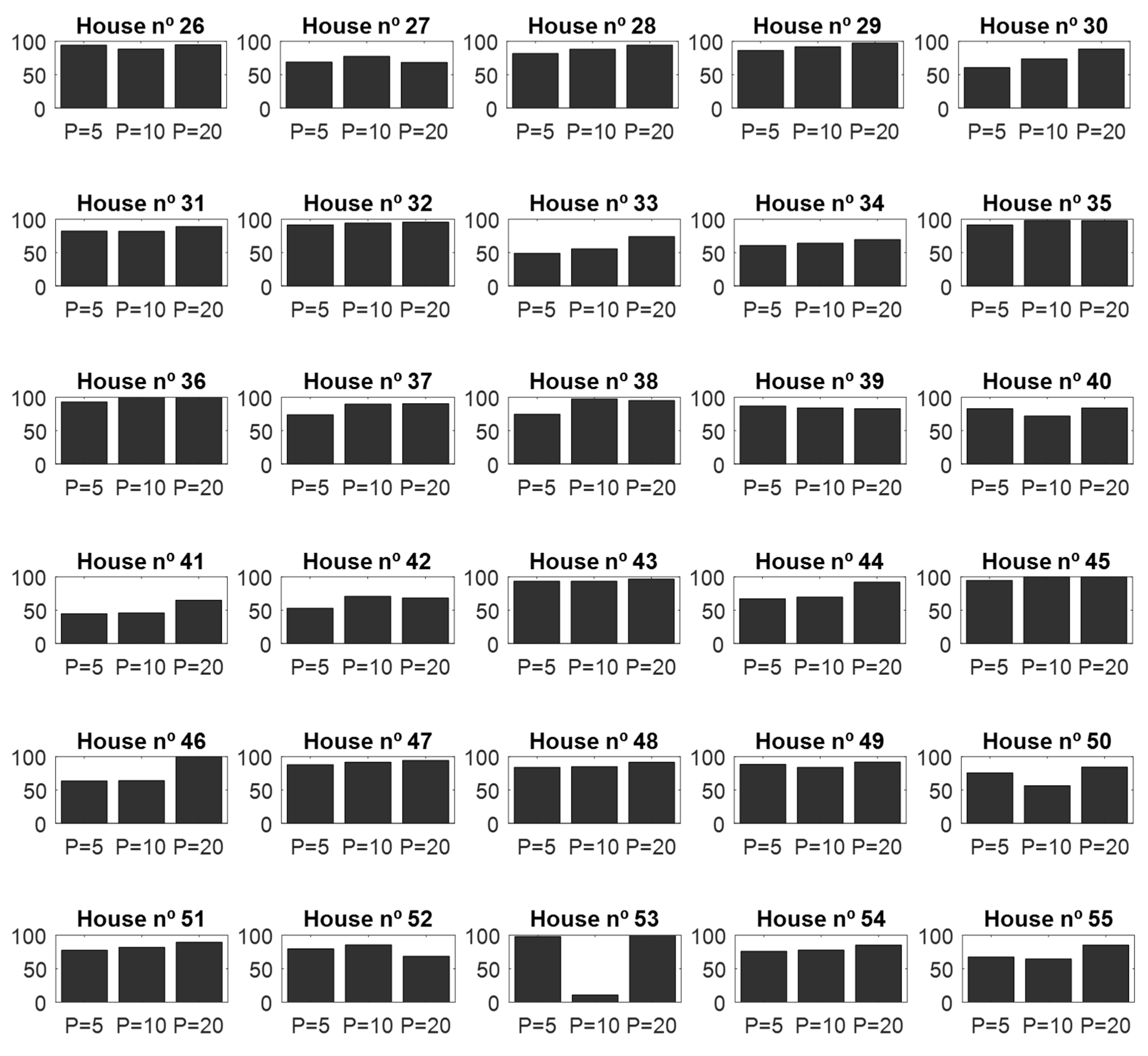
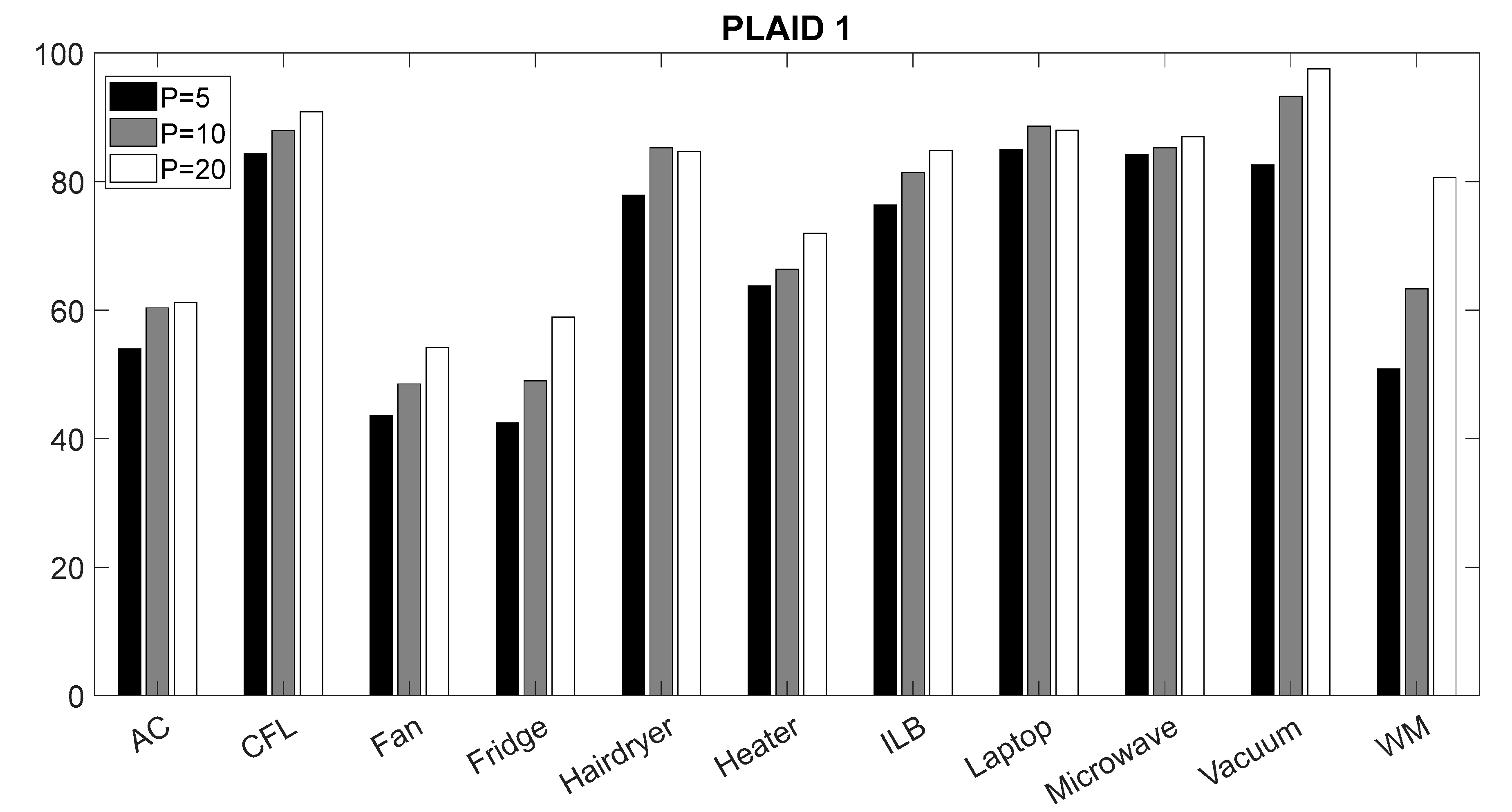
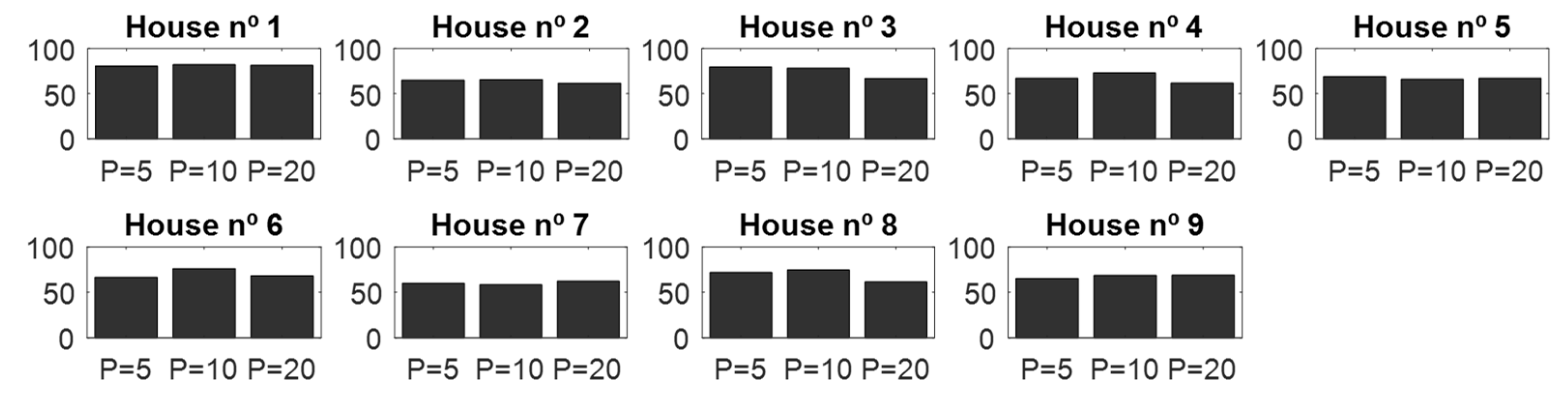
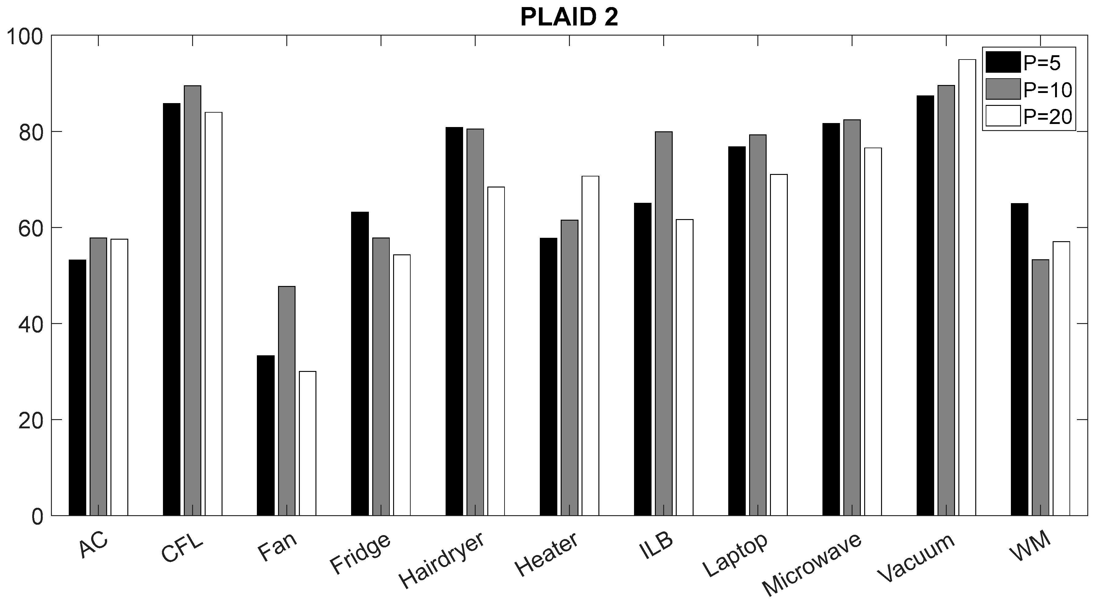
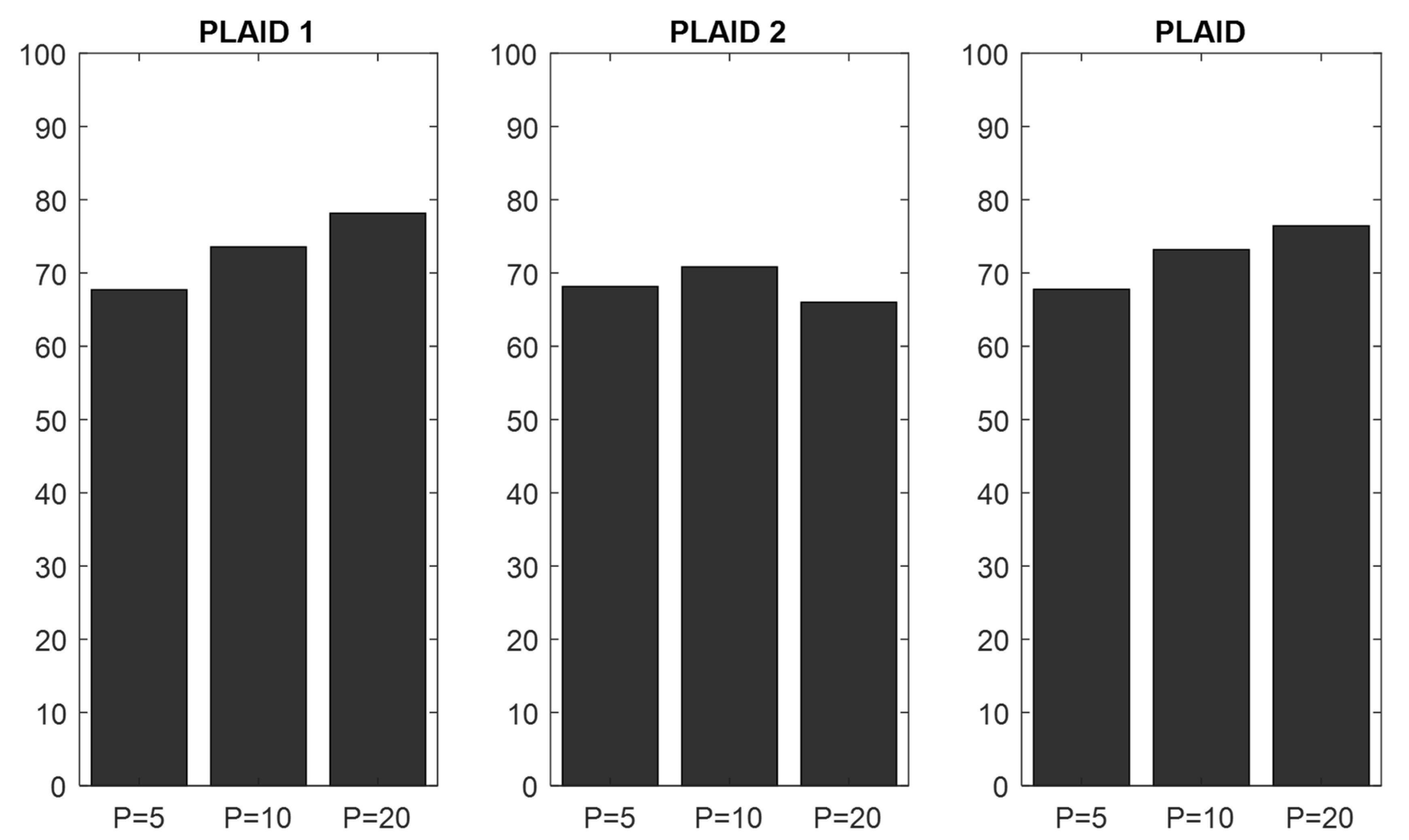
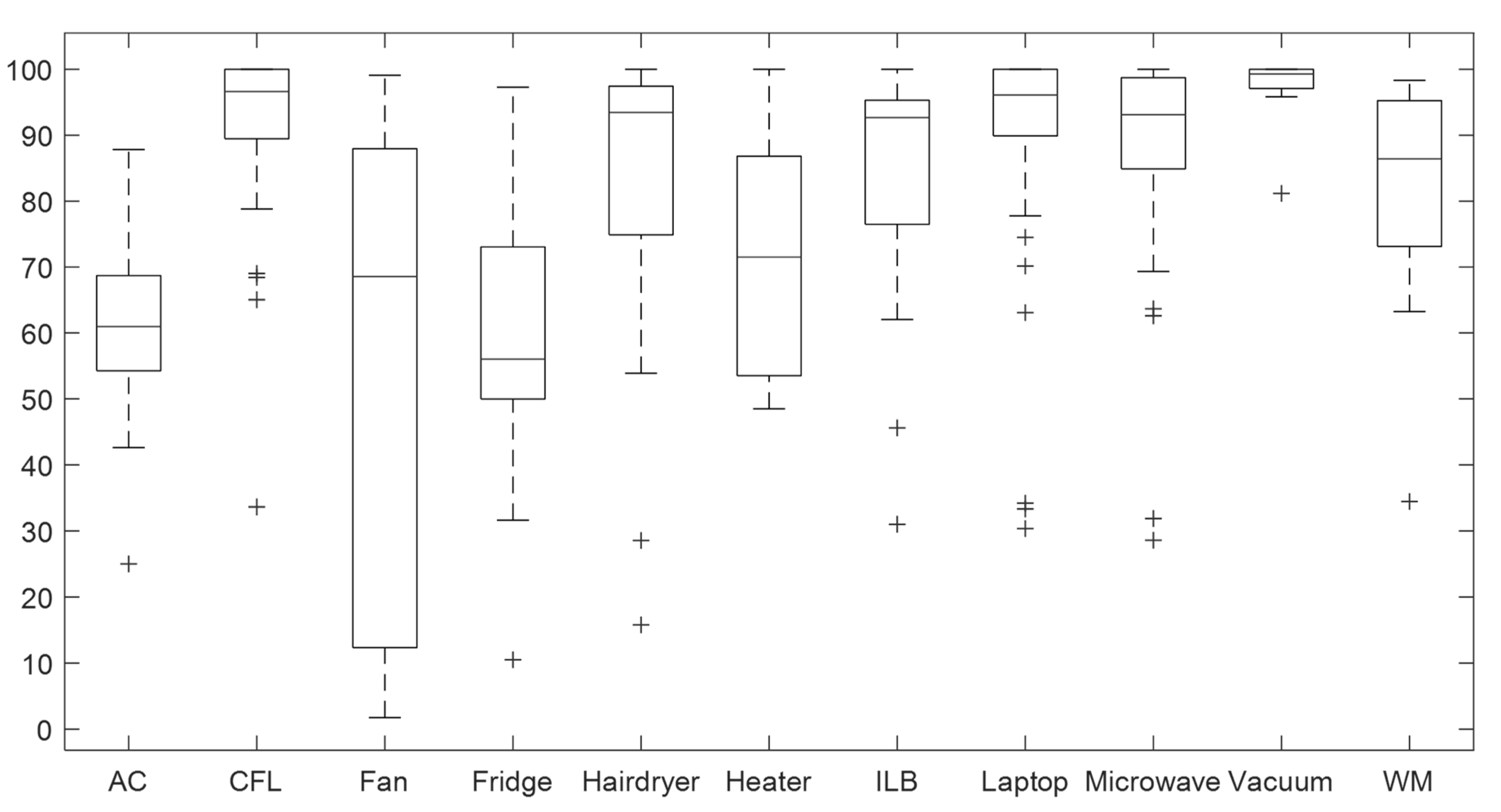
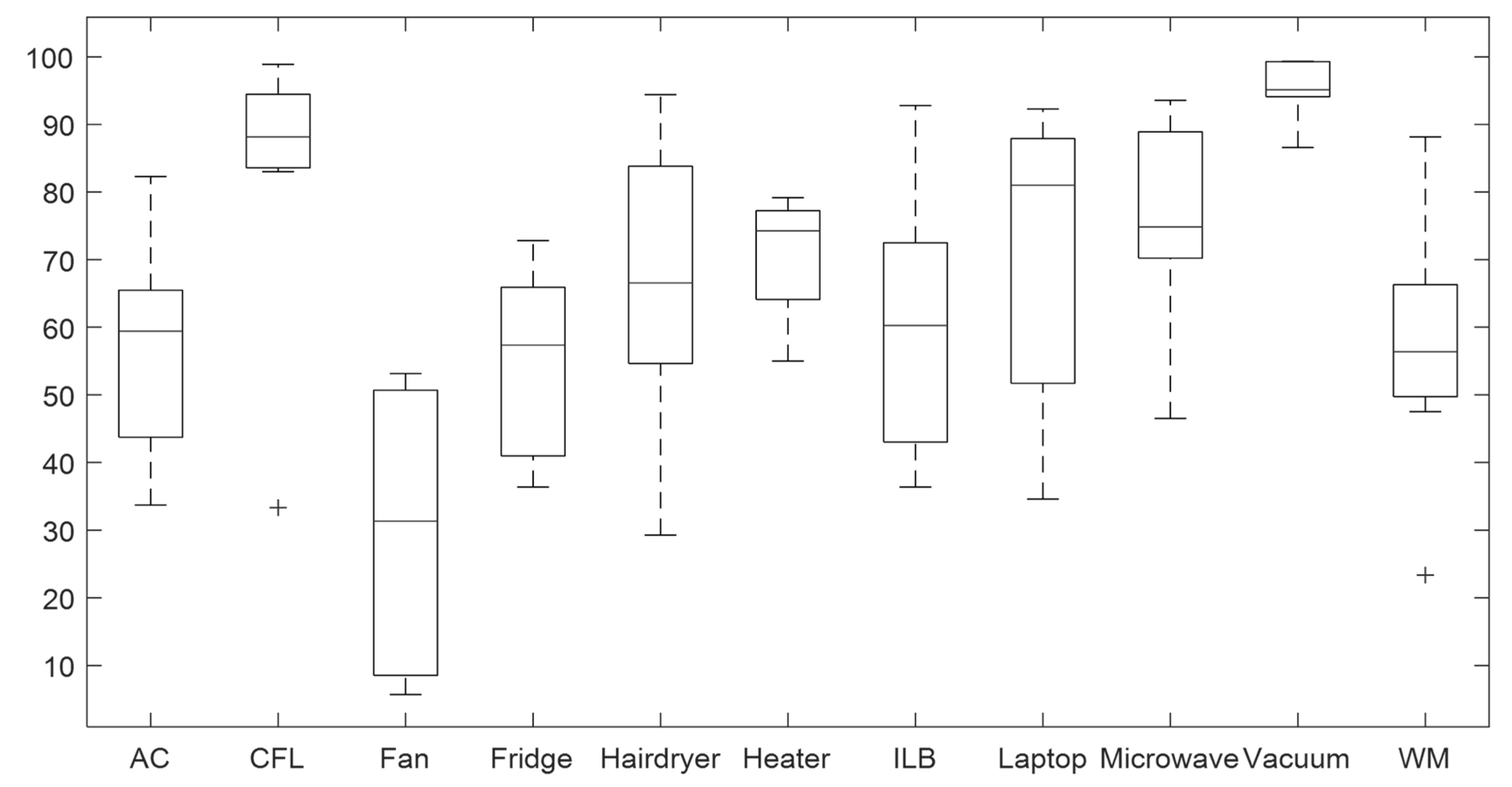
4.1. Validation of the CNN Classifier According to Window Sizes

Figure 5 and Figure 6 present the classification for PLAID 1 dataset of different windows size for each house and appliances, respectively. Figure 7 and Figure 8 present the classification for PLAID 2 of different windows size for each house and appliances, respectively. Figure 9 shows the overall F-score of PLAID 1 and PLAID 2 dataset. The mean F-score of combined dataset was done by weighted methods because the dataset PLAID 1 and PLAID 2 does not have equal number of houses. PLAID 1 and PLAID 2 are weighted according to their respective house numbers. For mean F-score it can be seen that, with the increasing of the window size, the F-score value of appliance classification from each house improves and, consequently, the F-score of the overall classification are also enhanced. The highest total F-score was achieved using a 333 ms window size (20 periods) hence in this work a 333 ms window is considered.

4.2. Performance and Cost

The parallelism was implemented in all multiplications/accumulations into the convolution layer and in all filters into the polling layer. Table 2 presents the required resources, performance and power consumption of the hardware implementation. These values have been obtained through the report from the Vivado.
Analyzing the Table 2, the design spent, mostly, LUT and BRAM for storing the kernel and weights values and for saving temporary the results of each layers. The DSPs are used to compute the basic operation of the CNN. The resulting resources are also used to implement counters and the controller through a state machine. The latency of this design is approximately 5.7 ms, which is lower than the window size (333 ms). Not only this implies that the classification is done before finishing the next window size but also it is possible to run overlapping window with 5.7 ms slide. To further complement our results, a performance using a CPU and a GPU have been measured. The CPU is an i7-Intel (4-core) with a clock speed of 4.20 GHz and a RAM of 32 GB. The GPU is a GeForce Nvidia GTX 1050 Nvidia 768 Compute Unified Device Architecture (CUDA) Cores. The performance were 69 ms using CPU and 87 ms using the GPU. In this case, it is assumed that CUDA has a start-up overhead because for small CNNs, like this one. To state more concretely, although the GPU bound code will run faster than the CPU code, the cost to transfer the data to and from the GPU will outweigh any gains from using the GPU. Consequently, since the transfer of data between CPU and GPU is a requirement of our application, GPU will not represent significant gains.

4.3. Comparison Results

Table 3 summarizes our F-score values using leave-one-house method and compares to recently publish results, using the same dataset, where available.
The obtained F-score value of the proposed system is compared to those of the ensembles classifiers [17] and the CNN classifier [9]. Comparing the proposed system with these two recent works, the proposed system presents a slightly higher F-score than the other CNN work. The proposed system has lower F-score value than the ensemble methods [17]. The model presented in [17] has an ensemble of 55 feed-forward neural network with 30 hidden neurons. If all hidden neurons are combined, the model would have 1650 neurons. Comparing this model with our model, our model is small. However, the proposed classifier presents a difference of 8% on the total F-score when compared with the model using a Neural Network Ensembles. This difference comes because the neural network ensemble classifies the appliances using the raw current and voltage waveforms as inputs instead of V-I trajectory. In the other hand, this difference comes mostly from the low F-score value of AC and fan. From our understanding, this misclassification is due to the similarities of V-I trajectories of these two appliances. This similarity comes of the fan which is coupled inside of an AC. In addition, the proposed model do not need any extra feature extraction method which also reduce the size of the implemented system. Furthermore, different from what has been developed in this work, the neural network ensemble classifies the appliances using the raw current and voltage waveforms as inputs instead of V-I trajectory.
Figure 10 and Figure 11 present box and whisker plots showing the median of F-score, the outliers and the 25th and 75th percentiles. Analyzing these figures, the appliances CFL and vacuum present the best F-score. On the other hand, the fan presents the worst F-score. Still, looking at Figure 10 and Figure 11, the result has fluctuations. The reason for that could be due to some houses do not have all appliances. In fact, the worst case is the fan where the F-score values fluctuate from 0% to 100%. This fluctuation contribute to decrease the overall score. Also, looking at the remaining appliances, the outliers presented in the remaining appliances have a negative contribution in the overall performance of the system.
Making a comparison between the developed local identification method and the on-line identification method, the proposed methods is advantageous. The disadvantage of the on-line identification method is the raw data needs to be transferred by internet into the classifier of appliances which is located on the cloud. Conversely, if the proposed method is used, only the answer of system will be sent through the internet. Thus, the compression ratio, r, is defined by:
  r = T r a n s m i s s i o n   u s i g n   r a w   d a t a T r a n s m i s s i o n   u s i g n   t h e   p r o p o s e d   m e t h o d   = f s × w i n d o w   s i z e   p e r i o d × 1 f g   T r a n s m i s s i o n   u s i g n   t h e   p r o p o s e d   m e t h o d    
Now, considering the sampling frequency, f s , of 30 kHz, the window size period of 20 to develop the classifier and the grid frequency,   f g , of 60 Hz in USA (50 Hz in EU). If the online identification method is used, 10,000 samples needed to be sent through the internet. Conversely, if the proposed method is used, only the answer of system will be sent through the internet. So, it is expected to reduce the communication bandwidth requirement about 4 orders of magnitude.

5. Conclusion and Future Work Directions

The present work proposes a strategy to identify appliances through analyzing changes in the voltage and current and deducing what appliances are used in the house as well as their individual energy consumption. A CNN, which can automatically extract relevant spatial features from the VI-trajectories, was proposed as a classifier for identifying appliances. The CNN was applied on the PLAID 1 and PLAID 2 dataset resulting in an F-score equal to 78.16% and 66.01%, respectively. The proposed system presents a slightly higher F-score than the CNN work found in the literature. However, the proposed classifier presents a difference of 8% on the total F-score when compared with the model using a Neural Network Ensembles. This difference comes because the neural network ensemble classifies the appliances using the raw current and voltage waveforms as inputs instead of V-I trajectory.
Also, in this paper, the CNN was implemented on hardware. The idea behind this implementation was getting the response of classifier before completing 333 ms (the window size extension). For this implementation, a Zynq board was used. The main advantage of this implementation is to execute the CNN, which is the most computationally intensive part, on an FPGA. The exploration of parallelism to speed up processing was extensively applied.
In the future, data collection methods are going to be implemented in the processing subsystem, as well as data transfer into the board. This is expected to reduce the communication bandwidth requirement about four orders of magnitude.
Likewise, considering the recent promise of GPU on SoC to rapidly deploys trained deep neural networks and accelerate their inference step, additional work should be conducted towards understanding if such system can become a reliable alternative to FPGAs in this or similar application scenarios.

Author Contributions

Conceptualization and Methodology: D.B., S.S.M., L.P.; Research and Formal Analysis: D.B., S.S.M.; Writing-original draft: D.B.; Writing-review & Editing: D.B., S.S.M., L.P., L.S., F.M.-D.

Funding

This work was supported by ARDITI–Agência Regional para o Desenvolvimento e Tecnologia under the scope of the Project M1420-09-5369-FSE-000001–PhD Studentship and by Portuguese national funds through FCT under project UID/CEC/50021/2013.

Acknowledgments

The authors thank to the anonymous reviewers for their constructive comments. Also, the authors wish to thank the dataset providers. The PLAID: The Plug Load Appliance Identification Dataset was obtained in: http://www.plaidplug.com/.

Conflicts of Interest

The authors declare no conflict of interest.

References

  1. Hart, G.W. Nonintrusive appliance load monitoring. Proc. IEEE 1992, 80, 1870–1891. [Google Scholar] [CrossRef]
  2. Armel, K.C.; Gupta, A.; Shrimali, G.; Albert, A. Is disaggregation the holy grail of energy efficiency? The case of electricity. Energy Policy 2013, 52, 213–234. [Google Scholar] [CrossRef] [Green Version]
  3. Esa, N.F.; Abdullah, M.P.; Hassan, M.Y. A review disaggregation method in Non-intrusive Appliance Load Monitoring. Renew. Sustain. Energy Rev. 2016, 66, 163–173. [Google Scholar] [CrossRef]
  4. Nalmpantis, C.; Vrakas, D. Machine learning approaches for non-intrusive load monitoring: from qualitative to quantitative comparation. Artif. Intell. Rev. 2018, 1–27. [Google Scholar] [CrossRef]
  5. Pereira, L.; Nunes, N. Performance evaluation in non-intrusive load monitoring: Datasets, metrics, and tools—A review. Wiley Interdiscip. Rev. Data Min. Knowl. Discov. 2018. [Google Scholar] [CrossRef]
  6. Gao, J.; Kara, E.C.; Giri, S.; Bergés, M. A feasibility study of automated plug-load identification from high-frequency measurements. In Proceedings of the 2015 IEEE Global Conference on Signal and Information Processing (GlobalSIP), Orlando, FL, USA, 14–16 December 2015; IEEE: Piscataway, NJ, USA, 2015; pp. 220–224. [Google Scholar]
  7. Lam, H.Y.; Fung, G.S.K.; Lee, W.K. A novel method to construct taxonomy electrical appliances based on load signatures. IEEE Trans. Consum. Electron. 2007, 53, 653–660. [Google Scholar] [CrossRef] [Green Version]
  8. Hassan, T.; Javed, F.; Arshad, N. An Empirical Investigation of V-I Trajectory Based Load Signatures for Non-Intrusive Load Monitoring. IEEE Trans. Smart Grid 2014, 5, 870–878. [Google Scholar] [CrossRef] [Green Version]
  9. De Baets, L.; Ruyssinck, J.; Develder, C.; Dhaene, T.; Deschrijver, D. Appliance classification using VI trajectories and convolutional neural networks. Energy Build. 2018, 158, 32–36. [Google Scholar] [CrossRef] [Green Version]
  10. Kostyk, T.; Herkert, J. Societal Implications of the Emerging Smart Grid. Commun. ACM 2012, 55, 34–36. [Google Scholar] [CrossRef]
  11. McLaughlin, S.; McDaniel, P.; Aiello, W. Protecting Consumer Privacy from Electric Load Monitoring. In Proceedings of the 18th ACM Conference on Computer and Communications Security; CCS ’11, Chicago, IL, USA, 17–21 October 2011; pp. 87–98. [Google Scholar]
  12. Barbosa, P.; Brito, A.; Almeida, H. A Technique to provide differential privacy for appliance usage in smart metering. Inf. Sci. 2016, 370–371, 355–367. [Google Scholar] [CrossRef]
  13. Cao, H.; Liu, S.; Wu, L.; Guan, Z.; Du, X. Achieving differential privacy against non-intrusive load monitoring in smart grid: A fog computing approach. Concurr. Comput. Pract. Exp. 2018. [Google Scholar] [CrossRef]
  14. Kolter, Z.; Matthew, J. REDD: A public data set for energy disaggregation research. In Proceedings of the Data Mining Applications in Sustainability (SustKDD), San Diego, CA, USA, 21 August 2011. [Google Scholar]
  15. Iksan, N.; Sembiring, J.; Haryanto, N.; Supangkat, S.H. Appliances identification method of non-intrusive load monitoring based on load signature of V-I trajectory. In Proceedings of the International Conference on Information Technology Systems and Innovation (ICITSI), Bandung, Indonesia, 16–19 November 2015; IEEE: Piscataway, NJ, USA, 2015; pp. 1–6. [Google Scholar]
  16. Gao, J.; Giri, S.; Kara, E.C.; Bergés, M. PLAID: A public dataset of high-resoultion electrical appliance measurements for load identification research. In Proceedings of the 1st ACM Conference on Embedded Systems for Energy-Efficient Buildings—BuildSys, Memphis, TN, USA, 3–6 November 2014; Volume 14, pp. 198–199. [Google Scholar]
  17. Barsim, K.S.; Mauch, L. Bin Neural Network Ensembles to Real-time Identification of Plug-level Appliance Measurements. In Proceedings of the 3rd International Workshop on Non-Intrusive Load Monitoring, Vancouver, BC, Canada, 14–15 May 2016. [Google Scholar]
  18. Du, L.; He, D.; Harley, R.G.; Habetler, T.G. Electric Load Classification by Binary Voltage-Current Trajectory Mapping. IEEE Trans. Smart Grid 2016, 7, 358–365. [Google Scholar] [CrossRef]
  19. De Baets, L.; Develder, C.; Dhaene, T.; Deschrijver, D. Automated classification of appliances using elliptical fourier descriptors. In Proceedings of the 2017 IEEE International Conference on Smart Grid Communications (SmartGridComm), Dresden, Germany, 23–27 October 2017; IEEE: Piscataway, NJ, USA, 2017; pp. 153–158. [Google Scholar]
  20. Kahl, M.; UI Haq, A.; Kriechbaumer, T.; Hans-Arno, J. WHITED—A Worldwide Household and Industry Transient Energy Data Set. In Proceedings of the 3rd International NILM Workshop, Vancouver, BC, Canada, 14–15 May 2016. [Google Scholar]
  21. Fukushima, K.; Miyake, S. Neocognitron: A new algorithm for pattern recognition tolerant of deformations and shifts in position. Pattern Recognit. 1982, 15, 455–469. [Google Scholar] [CrossRef]
  22. Mamalet, F.; Garcia, C. Simplifying ConvNets for fast learning. In Proceedings of the Lecture Notes in Computer Science (Including Subseries Lecture Notes in Artificial Intelligence and Lecture Notes in Bioinformatics), Rome, Italy, 10–14 September 2012; Volume 7553, LNCS. pp. 58–65. [Google Scholar]
  23. Goodfellow, I.; Bengio, Y.; Courville, A. Deep Learning; MIT Press: Cambridge, MA, USA, 2016. [Google Scholar]
  24. Ren, J.S.J.; Xu, L. On Vectorization of Deep Convolutional Neural Networks for Vision Tasks. In Proceedings of the AAAI'15 Twenty-Ninth AAAI Conference on Artificial Intelligence, Austin, TX, USA, 25–30 January 2015; pp. 1840–1846. [Google Scholar]
  25. Stutz, D. Understanding Convolutional Neural Networks. Nips 2016 2014, 1–23. [Google Scholar] [CrossRef]
  26. Nagi, J.; Ducatelle, F. Max-pooling convolutional neural networks for vision-based hand gesture recognition. In Proceedings of the 2011 IEEE International Conference on Signal and Image Processing Applications (ICSIPA), Kuala Lumpur, Malaysia, 16–18 November 2011; IEEE: Piscataway, NJ, USA, 2011; pp. 342–347. [Google Scholar] [CrossRef] [Green Version]
  27. Haykin, S. Neural Networks: A Comprehensive Foundation; Macmillan: New York, NY, USA, 1994; pp. 107–116. [Google Scholar]
  28. Memisevic, R.; Zach, C. Gated softmax classification. In Proceedings of the Advances in Neural Information Processing Systems 23 (NIPS 2010), Vancouver, BC, USA, 6–9 December 2010. [Google Scholar]
  29. Pereira, L.; Ribeiro, M.; Jardim, N. Engineering and deploying a hardware and software platform to collect and label non-intrusive load monitoring datasets. In Proceedings of the Sustainable Internet and ICT for Sustainability (SustainIT), Funchal, Portugal, 6–7 December 2017; pp. 1–9. [Google Scholar]
  30. Remscrim, Z.; Paris, J.; Leeb, S.B.; Shaw, S.R.; Neuman, S.; Schantz, C.; Muller, S.; Page, S. FPGA-based spectral envelope preprocessor for power monitoring and control. In Proceedings of the Twenty-Fifth Annual IEEE Applied Power Electronics Conference and Exposition (APEC), Palm Springs, CA, USA, 21–25 February 2010; IEEE: Piscataway, NJ, USA, 2010; pp. 2194–2201. [Google Scholar]
  31. Trung, K.N.; Zammit, O.; Dekneuvel, E.; Nicolle, B.; Van, C.N.; Jacquemod, G. An innovative non-intrusive load monitoring system for commercial and industrial application. In Proceedings of the 2012 International Conference on Advanced Technologies for Communications, Hanoi, Vietnam, 10–12 October 2012; IEEE: Piscataway, NJ, USA, 2012; pp. 23–27. [Google Scholar]
  32. LogiCORE IP Block Memory Generator v6.2; DS512; Xilinx: San Jose, CA, USA, 1 March 2011; Available online: https://www.xilinx.com/support/documentation/ip_documentation/blk_mem_gen/v6_2/blk_mem_gen_ds512.pdf (accessed on 12 September 2018).
  33. Säckinger, E.; Boser, B.E.; Jackel, L.D. A neurocomputer board based on the ANNA neural network chip. In Proceedins of the NIPS’91 4th International Conference on Neural Information Processing Systems, Denver, CO, USA, 2–5 December 1991; Morgan Kaufmann Publishers Inc.: San Francisco, CA, USA, 1991; pp. 773–780. [Google Scholar]
  34. Sackinger, E.; Boser, B.E.; Bromley, J.; LeCun, Y.; Jackel, L.D. Application of the ANNA Neural Network Chip to High-Speed Character Recognition. IEEE Trans. Neural Netw. 1992, 3, 498–505. [Google Scholar] [CrossRef] [PubMed]
  35. Säckinger, E.; Graf, H.P. A system for high-speed pattern recognition and image analysis. In Proceedings of the Fourth International Conference on Microelectronics for Neural Networks and Fuzzy Systems, Turin, Italy, 26–28 September 1994; IEEE: Piscataway, NJ, USA, 1994. [Google Scholar] [CrossRef]
  36. Korekado, K.; Morie, T.; Nomura, O.; Ando, H.; Nakano, T.; Matsugu, M.; Atsushi, I. A convolutional Neural Network VLSI for image Recognition Using Merged/Mixed Analoge-Digital Architecture. In Proceedings of the KES: Knowledge-Based Intelligent Information and Engineering, Oxford, UK, 3–5 September 2003; pp. 169–176. [Google Scholar]
  37. Fieres, B.; Grubl, A.; Philipp, S.; Meier, K.; Schemmel, J.; Schurmann, F. A Platform for Parallel Operation of VLSI Neural Networks. In Proceedings of the BICS, Scotland, UK, 29 August–1 September 2004. [Google Scholar]
  38. Farabet, C.; Poulet, C.; Han, J.Y.; LeCun, Y. CNP: An FPGA-based processor for Convolutional Networks. In Proceedings of the FPL 09: 19th International Conference on Field Programmable Logic and Applications, Prague, Czech Republic, 31 August–2 September 2009; IEEE: Piscataway, NJ, USA, 2009; pp. 32–37. [Google Scholar]
  39. Zhang, C.; Li, P.; Sun, G.; Guan, Y.; Xiao, B.; Cong, J. Optimizing FPGA-based Accelerator Design for Deep Convolutional Neural Networks. In Proceedings of the 2015 ACM/SIGDA International Symposium on Field-Programmable Gate Arrays—FPGA, Monterey, CA, USA, 22–24 February 2015; pp. 161–170. [Google Scholar]
  40. Baptista, D.; Sousa, L.; Morgado-Dias, F. Configurable N-fold Hardware Architecture for Convolutional Neural Networks. In Proceedings of the International Conference on Biomedical Engineering and Applications—ICBEA18, Funchal, Portugal, 9–12 July 2018. [Google Scholar]
  41. Ovtcharov, K.; Ruwase, O.; Kim, J.; Fowers, J.; Strauss, K.; Chung, E.S. Accelerating Deep Convolutional Neural Networks Using Specialized Hardware; Microsoft Research: Cambridge, UK, 2015. [Google Scholar]
  42. Cloutier, J.; Cosatto, E.; Pigeon, S.; Boyer, F.R.; Simard, P.Y. VIP: An FPGA-based processor for image processing and neural/nnetworks. Proceedings of Fifth International Conference on Microelectronics for Neural Networks, Lausanne, Switzerland, 12–14 February 1996; IEEE: Piscataway, NJ, USA, 1996; pp. 330–336. [Google Scholar] [CrossRef]
  43. Kingma, D.P.; Ba, J.L. Adam: A Method for Stochastic Optimization. In Proceedings of the 3rd International Conference for Learning Representations, San Diego, CA, USA, 7–9 May 2015. [Google Scholar]
  44. Zynq-7000 All Programmable SoC Data Sheet: Overview; DS190; Xilinx: San Jose, CA, USA, 2017; Volume 190.
  45. Mason, J.C.; Handscomb, D.C. Chebyshev Polynomials; Chapman & Hall/CRC Press LLC: Boca Raton, Florida, USA, 2003; ISBN 0849303559. [Google Scholar]
  46. Baptista, D.; Morgado-Dias, F. Low-resource hardware implementation of the hyperbolic tangent for artificial neural networks. Neural Comput. Appl. 2013, 23, 601–607. [Google Scholar] [CrossRef]
  47. Nascimento, I.; Jardim, R.; Morgado-Dias, F. Hyperbolic tangent implementation in hardware: A new solution using polynomial modeling of the fractional exponential part. Neural Comput. Appl. 2013, 23, 363–369. [Google Scholar] [CrossRef]
  48. Power Methodology Guide; UG786; Xilinx: San Jose, CA, USA, 2011; Volume 786, p. 54. Available online: https://www.xilinx.com/support/documentation/sw_manuals/xilinx13_1/ug786_PowerMethodology.pdf (accessed on 12 September 2018).
  49. Vivado Design Suite User Guide Design Analysis and Closure Techniques; UG906; Xilinx: San Jose, CA, USA, 2012; Volume 906, Available online: https://www.xilinx.com/support/documentation/sw_manuals/xilinx2017_3/ug906-vivado-design-analysis.pdf (accessed on 12 September 2018).
  50. Zynq-7000 All Programmable SoC DC and AC Switching Characteristics; DS191; Xilinx: San Jose, CA, USA, 2014; Volume 187, Available online: https://www.xilinx.com/support/documentation/data_sheets/ds187-XC7Z010-XC7Z020-Data-Sheet.pdf (accessed on 12 September 2018).
Figure 1. Diagram illustrating the system implementation using a Zynq-7000 device.
Energies 11 02460 g001
Figure 2. V-I trajectory of 11 appliances for three different window size. These pictures are created for visual purpose only actual input is a 50 × 50.
Energies 11 02460 g002
Figure 3. Design implemented. C: Calculation of the convolution; P: Calculation of the pooling; F: Calculation of the full output; K: Convolution Kernel; b: Bias; W: Weight.
Energies 11 02460 g003
Figure 4. Demonstrative diagram of the parallelism of the implementation: (a) multiplication/accumulation for convolving with a kernel k   2 × 2 ; (b) pooling assuming a filter belonging to   2 × 2 .
Energies 11 02460 g004
Figure 5. F-score values for each house from database plug load appliance identification dataset (PLAID) 1: x axis indicating the different periods and y axis is the F-score in percentage (%).
Energies 11 02460 g005aEnergies 11 02460 g005b
Figure 6. F-score values for each appliance from database PLAID 1: x axis indicating the different appliance and y axis is the F-score in percentage (%).
Energies 11 02460 g006
Figure 7. F-score values for each house from database PLAID 2: x axis indicating the different periods and y axis is the F-score in percentage (%).
Energies 11 02460 g007
Figure 8. F-score values for each appliance from database PLAID 2: x axis indicating the different appliance and y axis is the F-score in percentage (%).
Energies 11 02460 g008
Figure 9. F-score values for PLAID 1, PLAID2 and weighted F-macro-score for PLAID: x axis indicating the different periods and y axis is the F-score in percentage (%).
Energies 11 02460 g009
Figure 10. Box and whisker plot for PLAID 1: x axis indicating the different appliances and y axis is the F-score in percentage (%).
Energies 11 02460 g010
Figure 11. Box and whisker plot for PLAID 2: x axis indicating the different appliances and y axis is the F-score in percentage (%).
Energies 11 02460 g011
Table 1. Convolutional neural network (CNN) architecture developed.
LayerKernel/Pooling WindowLayer Size
Input -1@50X50
Convolution—stride 1 (C1)[4@3X3]4@48X48
Pooling—stride 2 (P1)[4@2X2]4@24X24
Convolution—stride 1 (C2)[6@3X3]6@22X22
Pooling—stride 2 (P2)[6@2X2]6@11X11
Convolution—stride 1 (C3)[18@3X3]18@9X9
Full out (F1)-11
Table 2. Performance, cost and power consumption of the field programmable gate array (FPGA) for the implemented CNN.
ResourcesLUT47.25% (25,138 of 53,200)
LUTRAM1.41% (246 of 17400)
FF13.05% (13,884 of 10,6400)
BRAM36.43% (51 of 140)
DSP71.82% (158 of 220)
BUFG3.13% (1 of 32)
Latency (ms)≅ 5.7
PowerDynamic (W)1.701
Device Static (W)0.167
Total On-Chip Power (W)1.868
Junction Temperature (°C)46.5
Thermal Margin (°C)38.5
Effective thermal resistance to air (°C/W)11.5
Note: LUT: Look-up Table; LUTRAM: Memory Look-up Table; FF: Flip-Flops; BRAM: Block of Memory; DSP: Digital Signal Processor; BUFG: Global Buffers.
Table 3. F-Score Comparison: Plug Load Appliance Identification Dataset (PLAID).
ApplianceConvolutional Neural Networks [9]Neural Network Ensembles [17]Our Classifier
PLAID 1PLAID 1PLAID 1PLAID 2
CFL95.60%69.8%90.86%83.96%
Fridge50.93%96.9%58.91%54.32%
Hairdryer79.76%74.1%84.70%68.40%
Microwave93.14%74.0%86.98%76.54%
AC46.65%92.6%61.20%57.55%
Laptop97.94%77.4%88.01%71.01%
Vacuum97.91%88.2%97.55%94.94%
ILB80.58%95.6%84.83%61.63%
Fan60.12%98.6%54.18%30.04%
WM68.82%96.1%80.62%57.02%
Heater82.23%89.4%71.92%70.67%
Total77.61%86.61%78.16%66.01%

