Occupancy-Based HVAC Control with Short-Term Occupancy Prediction Algorithms for Energy-Efficient Buildings


1
Energy and Transportation Science Division, Oak Ridge National Laboratory, Oak Ridge, TN 37831, USA
2
Computational Sciences and Engineering Division, Oak Ridge National Laboratory, Oak Ridge, TN 37831, USA
*
Author to whom correspondence should be addressed.
†
These authors contributed equally to this work.
Energies 2018, 11(9), 2427; https://doi.org/10.3390/en11092427
Submission received: 24 August 2018
/
Revised: 6 September 2018
/
Accepted: 6 September 2018
/
Published: 13 September 2018
(This article belongs to the Special Issue Intelligent Control in Energy Systems)
Abstract
:This study aims to develop a concrete occupancy prediction as well as an optimal occupancy-based control solution for improving the efficiency of Heating, Ventilation, and Air-Conditioning (HVAC) systems. Accurate occupancy prediction is a key enabler for demand-based HVAC control so as to ensure HVAC is not run needlessly when when a room/zone is unoccupied. In this paper, we propose simple yet effective algorithms to predict occupancy alongside an algorithm for automatically assigning temperature set-points. Utilizing past occupancy observations, we introduce three different techniques for occupancy prediction. Firstly, we propose an identification-based approach, which identifies the model via Expectation Maximization (EM) algorithm. Secondly, we study a novel finite state automata (FSA) which can be reconstructed by a general systems problem solver (GSPS). Thirdly, we introduce an alternative stochastic model based on uncertain basis functions. The results show that all the proposed occupancy prediction techniques could achieve around 70% accuracy. Then, we have proposed a scheme to adaptively adjust the temperature set-points according to a novel temperature set algorithm with customers’ different discomfort tolerance indexes. By cooperating with the temperature set algorithm, our occupancy-based HVAC control shows 20% energy saving while still maintaining building comfort requirements.
1. Introduction
1.1. Background of Research
More than 30% of building energy is consumed by HVAC systems, which usually operate on a fixed schedule predefined by building owners or operation managers. Currently, most existing building control systems still condition rooms with a set-point assuming maximum occupancy from early morning until late evening during weekdays. As a result, rooms are often needlessly over-conditioned, which may lead to a significant waste in energy consumption. Occupancy based controls, as a promising remedy for the aforementioned issue, can achieve significant energy savings by temporally matching the building energy consumption and building usage. This has the potential to reduce up to a third of HVAC energy consumption. Moreover, accurate and reliable occupancy detection is becoming a key enabler for demand-response HVAC control, which requires the capturing of occupancy changes in real time [1]. By taking advantage of occupancy information, we can reduce building energy consumption via optimized scheduling of HVAC [2], as well as shading blinds and natural ventilation to make effective use of available natural resources [3,4,5].
Even in the rare cases where occupancy information is integrated into the HVAC operation, only binary decisions (occupied or not) are made, with the actual number of occupants in the building is ignored. However, even under this binary case, [6] has discovered that there exists potential annual energy savings of 10–42% if actual occupancy information has been properly utilized. In actuality, the energy consumption of that building is dominated by the occupancy and related activities [7]. It follows that there exists optimal control parameters, based on the instantaneous number of humans in a building and their associated behaviors, with great energy savings potential.
In fact, occupancy in a building is stochastic both in time and space, which greatly affects actual power consumption for an individual zone or building. Consequently, this will not only affect our decisions for improving energy efficiency but also in implementing the advanced demand response (Typically peak-shaving applications in modern energy management systems [8,9]). The authors of [10,11] discovered that average occupancy level for commercial buildings is at most a third of its maximum designed-for occupancy. Thus, accurate occupancy-sensing data provides significant insight for an online adaptive HVAC control strategy utilizing to the exact number of occupants in a building over a certain time period [12,13,14]. Moreover, occupant behavior is well recognized as a dominant source of the discrepency between predicted and actual building performance, and developing accurate short-term occupancy prediction will greatly enhance implementation of realistic building energy modeling and control.
1.2. Literature Review
1.2.1. Occupancy Models
Despite a plethora of potential application scenarios, buildings’ occupancy modeling remains a cumbersome, error-prone and expensive process [15]. A through literature review for real-time occupancy detection and modeling in commercial buildings has been delivered in [16]. For occupancy modeling, various occupant behavior models have been developed in [17,18,19,20]. Moreover, such occupancy models have been integrated with operable windows, blinds, and lighting in EnergyPlus [19]. More recently, occupancy information has also been applied in Home Energy Management System (HEMS) using Markov-chain algorithms [21] or machine learning algorithms [22].
As previously mentioned, the uncertain occupancy information plays a central role in developing demand-driven HVAC control strategy. Due to the stochastic nature of occupancy, short-term prediction of it for individual rooms remains a challenging task. Previous occupancy modeling studies have focused on representing different detailedness of occupants’ behavior, such as binary data (i.e., presence and absence) [23], accurate discrete values (i.e., the number of occupants) [24], or continuous probability distributions [25]. All these models achieved a balanced trade-off between model accuracy and complexity, depending on the actual application scenario. Consequently, an appropriate modeling complexity must be chosen for any specific case.
1.2.2. Occupancy-Based Control
When provided accurate occupancy models, demand-driven control can utilize such information to coordinate real-time HVAC usage, reducing energy use and maintaining indoor thermal comfort in buildings [13,26,27,28,29]. It has been reported in [30] that a 75% energy savings can be achieved by using a robust design which is less sensitive to occupant variation. Further, when integrated with model-based control strategies, 42% energy savings have been achieved by using real-time occupancy data [1].
The main task of a traditional HVAC control system is to maintain temperature and indoor air quality within a desired comfort range while minimizing energy use. Current mainstream HVAC control practice depends on the choice of predefined dead-band values, which involves a significant amount of tedious tuning. In fact, this tuning has become increasingly challenging with the rising complexity of modern HVAC systems, particularly with regard to the uncertain characteristics of occupancy [31].
An alternative approach is to use the well-known model predictive control (MPC) approach, which takes into account weather and occupancy forecasts (as shown in Figure 1). At each sampling time, MPC minimizes the energy use by optimizing a plan for future HVAC operation based on predictions of the weather and occupancy for a future time horizon [31]. MPC has been widely applied in building climate control systems and has demonstrated promising energy savings as studies in [32,33] show.
1.3. Main Idea and Outline
We note here that most of the aforementioned techniques require an off-line training process using a large amount of collected measurement. However, the focus of our paper is to provide an alternative on-line strategy for short-term occupancy prediction. The proposed occupancy-based control framework aims to minimize the total HVAC energy consumption while maintaining a comfortable indoor environment in buildings by utilizing a non-fixed temperature setpoint for the HVAC controller. To accomplish this, we recall one efficient algorithm [34] for optimally assigning temperature set-point based on both real-time forecasts of occupancy information of the building. To determine the temperature set-points for the planning horizon, a novel temperature setpoint algorithm is introduced, where a discomfort tolerance index is also included. After determining the optimal future temperature set-points, it is further integrated with an MPC framework to complete the occupancy-based control strategy.
Statement of contributions:
Our contribution in this paper is threefold: Firstly, we design a suitable utility function alongside a temperature set algorithm to capture the trade-off between occupancy comfort and energy consumption. Secondly, we propose three different occupancy estimation algorithms that enable short-term stochastic modeling of occupancy in buildings. Finally, we analyze and validate energy-saving performance of the proposed techniques. Detailed comparisons are provided for energy consumptions both with various occupancy estimation algorithms, and without any occupancy information. As mentioned in [35], very few implementations of occupancy models in building simulation are reported. To the best knowledge of the authors, there exist few available guidelines or analysis utilizing predicted occupancy information for occupancy-based HVAC control techniques. This paper bridges the gap between reliable stochastic occupancy modeling and energy efficiency building simulation.
It is an extension of authors’ previous work [34], where a more powerful prediction algorithm—Uncertain Basis has been brought into the picture. Most importantly, we present novel quantified analysis for true energy savings with demand-based HVAC control strategy in this paper. Finally, some discussions are provided to better illustrate true energy-saving benefit by using the proposed demand-based control strategy.
The paper is structured as follows: Section 2 defines the mathematical problem under consideration and HVAC model we use. We also set up a temperature setpoint algorithm which could adaptively tune the temperature setpoint of the room based on the real occupancy information. Section 3 contains details about the occupancy prediction algorithms. Three different prediction techniques, especially the uncertain basis technique is introduced to predict the occupancy for the first time. Section 4 presents the simulation results regarding the estimation performance of all the aforementioned estimation algorithms. Finally, Section 5 draws the conclusions and ideas for future directions of development.
2. Problem Formulation
In order to use occupancy for demand-based HVAC control, we first must illustrate our HVAC model settings and control strategy. MPC is a class of algorithms designed to exploit building models and forecasts of interior and exterior disturbance signals. An MPC algorithm then computes open-loop optimal control actions by optimizing a cost function over a finite time horizon.
The reference temperature set point will serve as a bridge to relate occupancy prediction with MPC control strategy via the temperature set algorithm proposed in [34].
2.1. Building Thermal Model
In this section, we describe the typical one-dimensional resistance-capacitance (RC) model used in MPC design. The model stems from a physics-based continuous-time model, which captures the dynamics of indoor temperature, interior-wall surface temperature, as well as exterior-wall core temperature. This building thermal model has been widely applied in dozens of researches [32,36,37] for simulating residential and commercial buildings. It is described by
where the variables are defined in Table 1, and the parameter values are provided in Table 2.
The system states are , , and . The model inputs consist of control decision variables and exterior disturbance signals. The control decision variables are the demands sent to HVAC systems (with represents the cooling power, while corresponds to the heating power). The disturbances are and .
To translate the model into an MPC-friendly model, we must define the state vector x, the control signal vector u, and the environment stochastic disturbance vector as:
The continuous-time state-space model can then be described compactly as:
where
We then consider the discrete-time (sampled) version of Equation (1) described by
where k is the discrete-time index, and the parameters are computed from the continuous-time model parameters in Equation (2).
It should be mentioned that such state-space matrices can be easily generated for any given buildings through either physics-based or data-driven modeling techniques.
2.2. Baseline Control Strategy (or RBC)
The performance of the proposed adaptive control scheme will be compared with a baseline rule-based on/off control (RBC) scheme commonly used by thermostats in residential homes. These RBC algorithms represent the core logic behind the most popular mechanical and digital controls of thermostats in residential homes. Figure 2a,b describe the overall schemes for summer and winter cases, respectively. Basically, the RBC rules compare the indoor temperature T with a given reference temperature , which is allowed to drift by a cooling/heating dead band or , respectively.
2.3. System Model
The system states are the room air temperature , interior wall surface temperature , and exterior-wall core temperature . u represents the control input, which is heating power in this scenario ( comes as electrical power kW, since power conversion coefficients from heating load are absorbed in the model), and v is the outside disturbance including: the outdoor dry-bulb temperature , the approximated sky temperature , the internal load of space [W], and the solar radiation on the nodes [W]. All variables with subscripts H correspond to the HVAC.
The thermal model for any given building can then be described as:
where
- StatesInputs
- Disturbance
We assume the following constraints are imposed on the temperature and control inputs (for winter heating):
where means cooling (we can consider similar heating case when positive). It should be mentioned that sub-index k represents the kth time step. Additionally, we consider a variable speed HVAC system, where 0 represents HVAC totally OFF, and 1 () means working at the maximum heating (cooling) power. It should be mentioned that while the temperature comfort interval has been chosen by ASHRAE, it can be adjusted to any other values based on user’s preference.
2.4. Cost Function
In this MPC problem, we desire to minimize both the temperature deviation from the reference setpoints and the energy consumption while simultaneously enforcing a performance guarantee that ensures the indoor temperature always falls in a pre-defined comfort zone. We can assign set-points for all three temperature states, where represents the indoor temperature set-points (dominated by current and future occupancy information). Ultimately, our objective is to find the finite-horizon control sequences which minimize the following finite horizon objective function:
where (i.e., semi-definite positive matrices), (i.e., positive definite matrix), N is the prediction horizon, and
Thus, once we have accurate occupancy predictions available provided in Section 3, we can adaptively adjust temperature set-points according to the novel temperature set algorithm proposed in [34]. From this, we will be able to achieve occupancy-based optimal control (as shown in Figure 3) to improve energy efficiency of the buildings.
2.5. Temperature Set Algorithm
In conventional practice, the HVAC operates under a fixed dead-band (chosen by the users) for indoor temperature. Currently, most temperature set-points are predefined by the building owner or administrator, and do not change frequently during the regular operation periods.
We recall our own simple yet effective algorithm (shown in Algorithm 1) to assign reference temperature set-points for each half hour of the day based on the real-time occupancy [34]. Inside this temperature set algorithm, we need first define the maximum (max()) and minimum(min()) occupancy values (based on previous field measurement or survey) during normal operation. Similarly, we also must define the comfort band chosen by the customers. Obviously, the larger the band is, the more energy savings will be achieved. The beauty of Algorithm 1 is its ability to identify a temperature set-point depending on the occupancy information. The temperature set-points are then assigned to each half hour of the day based on the range in which the occupancy number of corresponding half hours fall in.
Following [38], a discomfort tolerance index is defined to characterize building users’ different choices/tolerance on thermal comfort (discomfort). Discomfort tolerance is considered high when , and low when .
| Algorithm 1 Temperature Setting Algorithm [34] |
|
3. Occupancy Prediction Algorithms
In this section, we introduce our algorithm for the detailed estimation of future occupancy, and we show how we could predict the number of occupants in the room. An overview of all the developed algorithms is summarized in Figure 4.
In order to study a practical occupancy model, we collected real occupancy data from an occupancy sensor for a room. We randomly pick a segment of data dated “13 October 2010–5 April 2011”, i.e., 174 days. The sampling interval is 30 min, so each individual sensor collects 48 occupancy samples each day. i.e., we have 8352 samples for each sensor. For simplicity, we consider the 8352 samples from a single sensor.
Natural questions which arise are: what is the probability for this room to be occupied; and how many people will be in the room?
To answer the first question, we could compute the probability for the room to be occupied by observing historic data. This has been reported in our earlier paper [34], so we skip this model here due to space constraints.
For the second problem, we need to apply more intelligent techniques (proposed in Section 3.1, Section 3.2, Section 3.3, Section 3.4 and Section 3.5) to predict the number of people in the room.
Due to occupancy’s stochastic characteristic, it is not realistic to expect the real occupancy of the room to exactly follow the given schedule. Therefore, we should desire to accurately predict the occupancy information based on the most recent measurement. Moreover, detailed occupancy estimation considers not only whether the building is occupied or not, but also takes into account the number of occupants in the building. Here we will introduce some background and several alternative techniques that may be adequate for occupancy estimation.
3.1. Expectation Maximization (EM)
The first occupancy modeling algorithm relies on the state-space model, which has been very popular in both societies of control systems and signal processing due to its advantage of on-line recursive implementation. The EM algorithm is a data-driven approach that builds and updates the estimated occupancy relying purely on collected measurements. Its core mechanism consists of two simple equations, i.e., a state Equation (7) and a measurement Equation (8).
A standard EM model in discrete time can be written as:
where ( denotes the space of real vectors with dimension ) is the state that characterizes the occupancy; it is a variable of the time series determined by the previous state and the noise term introduced at each k. and are corresponding coefficients.
The beauty of the EM algorithm is the time varying nature inherited in the state-space model, which enables the model to adapt dynamically to the most recent occupancy model. Moreover, it takes into account the noise terms and that capture small perturbations or uncertainties introduced at each time k. This greatly alleviates the challenges associated with occupancy uncertainties in the model.
3.2. Finite State Automata (FSA)
Probabilistic FSA [41] have previously been introduced to describe distributions over strings. FSA has been used quite successfully to address several complex sequential pattern recognition problems, such as continuous speech recognition, computational biology [42] and linguistics [43]. The general Systems Problem Solver (GSPS) proposed in [44], provides a novel and highly effective method for reconstructing the input/output behavior of FSA. The detailed algorithm and system formulation can be found in [45].
Given a system and a sequence of length n generated by that system, we may posit a relation between its variables. This relation takes the form of a function f that maps observations of some variables at times with to observations of other variables at time n.
In this occupancy problem, we want to know the exact number of people in the room. So we assume different numbers of occupants as different states in the FSA. As long as finite states are involved, the general form of the rule and the methods for constructing and forecasting are the same.
Such a relation is called a rule. Typically this purpose is forecasting; i.e., to predict future observations from past and current observations. This relation takes the form of a function f that maps observations of some variables at times to observations of other variables at time t. Rules are posited by the observer for some particular purpose.
Continuing the example above, consider strings comprised of the letters a, b, c. Take these strings to be our system and the variable to be a single character in a string. Observations of this variable are indexed by position in the string ordered from left to right so that the first character in the string is , the second is , and so forth. One example of a sequence for this system is .
A possible rule that predicts the next letter in this string is . This rule relates the characters in subsequences of length two such that the leftmost character predicts the rightmost character. Interpreting the sequence with this rule yields the following function: which occurs three times, which occurs three times, and which occurs two times.
3.3. Simplified Binary States FSA
In general, the length of the “look back depth” used is decided by actual problem. For our specific occupancy prediction problem, the system of interest has a single variable with two possible values: occupied (b) or not occupied (a). After tail and error check, we posit a rule that looks back three steps and also considers the time of day, i.e., . The time of day is used to characterize the different rules for different time period during a day; for the available data use there are 48 times that can be considered, as the sampling interval of the sensor is 30 min. Given the data and a rule, we can build a model for forecasting with the simple procedure described by Klir [44]. More details about working mechanisms for FSA can be found in [34].
To illustrate this procedure, consider the mask and sequence in Table 3. The system that generated this sequence has time variable and a single variable v that can take the value b or a. The rule for this mask built with 3000 data points is shown in Table 4. It should be noted that in order to simplify the explaination, we decouple the time variable from the rule. To be specific, Table 4 represents the rule for 3:00 p.m. using 3000 data points. Considering the sampling interval is every 30 min, we could generate 48 such rule tables for the whole day (24 h).
To illustrate how this model is applied for forecasting, suppose we begin with the latest observation sequence as at 3:00 p.m. The next output is a with probability or b with probability . If we were at a different time step other than 3:00 p.m., then the output is selected according to the corresponding rule table at that time step. Once the time step is fixed, then the second output is a with some probability p or b with probability . Continuing in this fashion, we can construct a tree of possible futures and use these possible futures to inform the control system.
3.4. Estimating Number of Occupants
We consider three methods for anticipating the actual number of occupants within a room.
FSA with 3 or More Input/Output Values
Though the method described in Section 3.3 only involves two states, it is readily extended to estimate the exact number of occupancy by using the number of occupants as variable rather than the binary occupied/unoccupied.
In the following simulation results, we show that the discussion for the binary model applies directly to the model with multiple states.
3.5. Basis Function
Finally, we introduce the third powerful algorithm, i.e., the uncertain basis functions. If we consider as the current occupancy measurements detected by occupancy sensor, it can be well represented by the following basis functions:
where are the basis functions, and , and is the corresponding coefficient of each basis function [46,47].
However, this trivial representation may not be able to capture all the dynamics of occupancy due to the limitation of fixed basis functions, which eliminates the uncertainty nature. An alternative way to cast this formulation is to assume that each basic function depends on some unknown parameter vectors , where only some statistics of the distribution of are known. Then, the corresponding coefficients can be estimated by minimizing an expected cost function following the technique developed in [48].
Following [48], we assume that each is independent. The basic functions are further represented by . The main objective here is to find the best coefficients to minimize the expected cost function defined as:
where is the expectation with respect to . The measured values are real, so we could estimate the coefficients following steps presented in [39].
We focus on predicting future occupancy using the basis function:
This means that we can predict occupancy values with p random basis functions. Similarly as in [39], we assume the basis functions to be governed by three different distributions, i.e., Gaussian, Laplace and Uniform. Consequently, we are able to compute occupancy predictions under each distribution.
4. Case Studies
To illustrate the effectiveness of the occupancy prediction techniques proposed in the last section, we assess their performance using the aforementioned occupancy measurement (at the beginning of Section 3). In the first part, performance of three occupancy prediction techniques are examined, and corresponding accuracy comparison are provided. In the second part, different temperature set trajectories s are obtained using our temperature set algorithm. The algorithm is employed to assign reference temperature set-points for each hour of the day. Lastly, these reference temperature set-points are utilized in the standard HVAC control strategies. In essence, different energy saving benefits are studied for traditional ON/OFF control and advanced MPC control, respectively.
4.1. Definition of the Performance Indexes
We define the estimation accuracy as the total number of correct predictions divided by the total number of predictions. The Root Mean Squared Error (RMSE), which characterizes the absolute estimation errors.
More formally, if we let ACC represent the accuracy, then using indicator functions, we obtain the accuracy of the estimator:
where O and are true and estimated occupancy, respectively. Let us denote the characteristic function of estimation error as:
Here, the RMSE is defined as the square root of the mean square error:
Therefore, RMSE will be the square root of (15).
4.2. Occupancy Prediction Performance
4.2.1. GSPS Model
In this GSPS-based scenario, we assume we have access to a large enough historical data set. We trained the model using the last 3000 and 5000 data points, respectively. The prediction results are shown in Figure 5a,b. As expected, the more data involved in training the FSA, the better the prediction results. This is also confirmed by the estimation error comparison shown in Table 5.
4.2.2. EM Method
Next, the elegant EM algorithm is applied to occupancy prediction. The performance is depicted in Figure 6, where only the last 20 sample points are used to predict the occupancy information at the very next time step.
4.2.3. Uncertain Basis Functions
In order to the show robustness of the proposed uncertain basis technique, we tested it with three different distributions for . It should be mentioned that only 10 last sampling points are used to build the optimal basis for each distribution. Figure 7 shows prediction comparison results using three different distributions.
4.3. Temperature Set Points
Through the above simulation results, we achieve the desired occupancy prediction. However, our goal is to design temperature set-points based on these occupancy sequences. In order to further determine the effectiveness of these occupancy prediction results, we integrate the occupancy prediction results into the temperature set algorithms. The one corresponding to basic functions using uniform distribution is presented in Figure 8.
4.4. Occupancy-Based Control
To show the energy-saving performance using the proposed stochastic models for occupancy and temperature set algorithm, we insert the obtained temperature reference into simple ON/OFF switching control framework. A fixed reference temperature is chosen for the baseline scenario. An occupancy-dependent reference temperature generated via our temperature set algorithm replaces original fixed schedule. This simple step will adaptively tune the set-point of HVAC systems according to current occupancy information, avoiding wasting energy for empty rooms.
In order to quantify the performance using different algorithms, we utilize the energy cost using traditional ON/OFF control strategy without any occupancy information as a benchmark. It should be mentioned that energy cost is defined as 2-norm, i.e., .
Next, a comparison between different algorithms is made by changing only the occupancy information. Detailed numerical result is given in the right end column of Table 5. We are expected to save approximately 13% and 20% energy consumptions for traditional ON/OFF and MPC control strategies, respectively.
4.5. Summary of the Results
In this section we compare four occupancy prediction algorithms, all trained using the same training set described at the beginning of Section 3. Figure 8 shows the realizations of occupancy predictions can be applied to the corresponding test set. Ideally, we can increase temperature set point when less occupants will be present in the room. As expected, we notice higher temperature set points are achieved corresponding to a larger tolerance index, as we are studying a summer cooling case in this paper. Table 5 summarizes the achieved numerical performance and accuracy comparison for the three algorithms. Generally speaking, both EM and Uncertain basis methods can provide reliable predictions with just a few historical data points. The GSPS method meanwhile, requires many more points to build a reliable model. Additionally, GSPS and Uncertain basis methods achieve a higher accuracy, while the EM method provides a degraded prediction result. Each method may find its own suitable application scenarios depending on the accuracy requirement and data structure.
It should be remarked that, although some mismatches exist for non-zero jumps in Figure 5a, Figure 6 and Figure 7c, all prediction algorithms track the 0 base line (non-occupied status) perfectly. Therefore, all prediction techniques are effective for identifying empty rooms, with an over 90 percent accuracy rate. Moreover, the accuracy conditions we set are extremely restrictive. In other words, the accuracy is said to be satisfied only when the estimated number of occupants is exactly the same as the real measurement. So in this case, the accuracy is void if the estimated number is 13 while actual number is 12.
Furthermore, the obtained occupancy status is successfully applied into the temperature set algorithm which dominates energy consumption in building climate systems. In this final experiment, we applied the designed temperature setpoints into two different algorithms - basic control and MPC (designed in Section 2), and compare their energy consumption. The building thermal zone model we picked has also been introduced in Section 2. The detailed energy consumption data of the simulation has been given in Table 6. These control tests complete our occupancy-based control framework, which showcases up to 20% energy saving benefits via the proposed corresponding control framework.
5. Conclusions and Future Work
In this paper, we propose three different occupancy prediction methods for demand-based HVAC control. All three proposed short-term stochastic modeling methods, GSPS, EM and uncertain basis, achieved more than 70% accuracy in the experimental studies. Furthermore, we have designed a novel temperature set algorithm to correctly assign temperature set points based on the instantaneous occupancy information. To complement the occupancy-based framework, we have integrated the temperature set point naturally into the MPC algorithm. Finally, detailed comparisons are provided for energy consumptions with various occupancy estimation algorithms and without any occupancy information. This paper delivered a novel end-to-end solution, which connects a reliable stochastic occupancy modeling study with the occupancy-based control design. Consequently, we have seen up to 20% energy saving by integrating the proposed technique into two standard HVAC control strategies.
A great number of increasingly complex models are being developed for HVAC systems. However, the limited number of implementations of such models in demand-based control and the lack of occupants’ effects limits their ability to improve efficiency while guaranteeing a comfortable temperature environment in buildings. Our near future work will involve detailed internal heat gain subject to different occupancy situations and various application scenarios, particularly the hot topic of building-to-grid integration. Another interested direction is to perform the sensitivity analysis for changing the set point. Basically, to answer the question, when is the best time to change the set-point; and how long/much will the electricity consumption reflect the change. This knowledge is critical for doing demand-response using buildings.
Author Contributions
Conceptualization, J.D., T.K. and J.N.; Methodology, J.D., T.K. and J.N.; Software, J.D. and C.W.; Validation, J.D. and C.W.; Formal Analysis, J.D. and T.K.; Investigation, J.D. and T.K.; Writing—Original Draft Preparation, J.D.; Writing—Review & Editing, J.N. and J.D.
Acknowledgments
This manuscript has been authored by UT-Battelle, LLC under Contract No. DE-AC05-00OR22725 with the U.S. Department of Energy. This material is based upon work supported by the U.S. Department of Energy. The United States Government retains and the publisher, by accepting the article for publication, acknowledges that the United States Government retains a non-exclusive, paid-up, irrevocable, world-wide license to publish or reproduce the published form of this manuscript, or allow others to do so, for United States Government purposes. The Department of Energy will provide public access to these results of federally sponsored research in accordance with the DOE Public Access Plan (http://energy.gov/downloads/doe-public-access-plan).
Conflicts of Interest
The authors declare no conflict of interest.
References
- Erickson, V.L.; Carreira-Perpiñán, M.Á.; Cerpa, A.E. Occupancy modeling and prediction for building energy management. ACM Trans. Sens. Net. 2014, 10, 42. [Google Scholar] [CrossRef]
- Sun, B.; Luh, P.B.; Jia, Q.S.; Jiang, Z.; Wang, F.; Song, C. Building energy management: Integrated control of active and passive heating, cooling, lighting, shading, and ventilation systems. IEEE Trans. Automation Sci. Eng. 2013, 10, 588–602. [Google Scholar]
- Tzempelikos, A.; Athienitis, A.K. The impact of shading design and control on building cooling and lighting demand. Solar Energy 2007, 81, 369–382. [Google Scholar] [CrossRef]
- Van Moeseke, G.; Bruyère, I.; De Herde, A. Impact of control rules on the efficiency of shading devices and free cooling for office buildings. Build. Environ. 2007, 42, 784–793. [Google Scholar] [CrossRef]
- Valdiserri, P.; Biserni, C.; Garai, M. Energy performance of a ventilation system for an apartment according to the Italian regulation. Inter. J. Energy Environ. Engin. 2016, 7, 353–359. [Google Scholar] [CrossRef]
- Erickson, V.L.; Carreira-Perpiñán, M.Á.; Cerpa, A.E. OBSERVE: Occupancy-based system for efficient reduction of HVAC energy. In Proceedings of the 10th ACM/IEEE International Conference on Information Processing in Sensor Networks, Chicago, IL, USA, 12–14 April 2011; pp. 258–269. [Google Scholar]
- Shih, H.C. A robust occupancy detection and tracking algorithm for the automatic monitoring and commissioning of a building. Energy Build. 2014, 77, 270–280. [Google Scholar] [CrossRef]
- Sharma, I.; Dong, J.; Malikopoulos, A.A.; Street, M.; Ostrowski, J.; Kuruganti, T.; Jackson, R. A modeling framework for optimal energy management of a residential building. Energy Build. 2016, 130, 55–63. [Google Scholar] [CrossRef]
- Dong, J.; Olama, M.M.; Kuruganti, T.; Nutaro, J.; Xue, Y.; Sharma, I.; Djouadi, S.M. Adaptive building load control to enable high penetration of solar photovoltaic generation. In Proceedings of the Power & Energy Society General Meeting IEEE, Chicago, IL, USA, 16–20 July 2017; pp. 1–5. [Google Scholar]
- Rafsanjani, H.N.; Ahn, C.R.; Alahmad, M. A review of approaches for sensing, understanding, and improving occupancy-related energy-use behaviors in commercial buildings. Energies 2015, 8, 10996–11029. [Google Scholar] [CrossRef]
- Brandemuehl, M.J.; Braun, J.E. The impact of demand-controlled and economizer ventilation strategies on energy use in buildings. ASHRAE Trans. 1999, 105, 39. [Google Scholar]
- Harle, R.K.; Hopper, A. The potential for location-aware power management. In Proceedings of the 10th international conference on Ubiquitous computing, Seoul, Korea, 21–24 September 2008; pp. 302–311. [Google Scholar]
- Erickson, V.L.; Cerpa, A.E. Occupancy based demand response HVAC control strategy. In Proceedings of the 2nd ACM Workshop on Embedded Sensing Systems for Energy-Efficiency in Building, Zurich, Switzerland, 3–5 November 2010; pp. 7–12. [Google Scholar]
- Garg, V.; Bansal, N. Smart occupancy sensors to reduce energy consumption. Energy Build. 2000, 32, 81–87. [Google Scholar] [CrossRef]
- Nguyen, T.A.; Aiello, M. Energy intelligent buildings based on user activity: A survey. Energy Build. 2013, 56, 244–257. [Google Scholar] [CrossRef] [Green Version]
- Labeodan, T.; Zeiler, W.; Boxem, G.; Zhao, Y. Occupancy measurement in commercial office buildings for demand-driven control applications—A survey and detection system evaluation. Energy Build. 2015, 93, 303–314. [Google Scholar] [CrossRef]
- Gunay, H.B.; O’Brien, W.; Beausoleil-Morrison, I. A critical review of observation studies, modeling, and simulation of adaptive occupant behaviors in offices. Build. Environ. 2013, 70, 31–47. [Google Scholar] [CrossRef]
- Parys, W.; Saelens, D.; Hens, H. Coupling of dynamic building simulation with stochastic modelling of occupant behaviour in offices–a review-based integrated methodology. J. Build. Perform. Simul. 2011, 4, 339–358. [Google Scholar] [CrossRef]
- Gunay, H.B.; O’Brien, W.; Beausoleil-Morrison, I. Implementation and comparison of existing occupant behaviour models in EnergyPlus. J. Build. Perform. Simul. 2016, 9, 567–588. [Google Scholar] [CrossRef]
- Yang, J.; Santamouris, M.; Lee, S.E. Review of occupancy sensing systems and occupancy modeling methodologies for the application in institutional buildings. Energy Build. 2016, 121, 344–349. [Google Scholar] [CrossRef]
- Louis, J.N.; Caló, A.; Leiviskä, K.; Pongrácz, E. Modelling home electricity management for sustainability: The impact of response levels, technological deployment & occupancy. Energy Build. 2016, 119, 218–232. [Google Scholar] [Green Version]
- Peng, Y.; Rysanek, A.; Nagy, Z.; Schlüter, A. Using machine learning techniques for occupancy-prediction-based cooling control in office buildings. Appl. Energy 2018, 211, 1343–1358. [Google Scholar] [CrossRef]
- Chaney, J.; Owens, E.H.; Peacock, A.D. An evidence based approach to determining residential occupancy and its role in demand response management. Energy Build. 2016, 125, 254–266. [Google Scholar] [CrossRef]
- Wang, W.; Chen, J.; Huang, G.; Lu, Y. Energy efficient HVAC control for an IPS-enabled large space in commercial buildings through dynamic spatial occupancy distribution. Appl. Energy 2017, 207, 305–323. [Google Scholar] [CrossRef]
- D’Oca, S.; Hong, T. Occupancy schedules learning process through a data mining framework. Energy Build. 2015, 88, 395–408. [Google Scholar] [CrossRef] [Green Version]
- Scott, J.; Bernheim Brush, A.; Krumm, J.; Meyers, B.; Hazas, M.; Hodges, S.; Villar, N. PreHeat: controlling home heating using occupancy prediction. In Proceedings of the 13th international conference on Ubiquitous computing, Beijing, China, 17–21 September 2011; pp. 281–290. [Google Scholar]
- Lu, J.; Sookoor, T.; Srinivasan, V.; Gao, G.; Holben, B.; Stankovic, J.; Field, E.; Whitehouse, K. The smart thermostat: using occupancy sensors to save energy in homes. In Proceedings of the 8th ACM Conference on Embedded Networked Sensor Systems, Zurich, Switzerland, 3–5 November 2010; pp. 211–224. [Google Scholar]
- Gunay, H.B.; O’Brien, W.; Beausoleil-Morrison, I. Development of an occupancy learning algorithm for terminal heating and cooling units. Build. Environ. 2015, 93, 71–85. [Google Scholar] [CrossRef]
- Peng, Y.; Rysanek, A.; Nagy, Z.; Schlüter, A. Occupancy learning-based demand-driven cooling control for office spaces. Build. Environ. 2017, 122, 145–160. [Google Scholar] [CrossRef]
- Karjalainen, S. Should we design buildings that are less sensitive to occupant behaviour? A simulation study of effects of behaviour and design on office energy consumption. Energy Efficiency 2016, 9, 1257–1270. [Google Scholar] [CrossRef]
- Oldewurtel, F.; Sturzenegger, D.; Morari, M. Importance of occupancy information for building climate control. Appl. Energy 2013, 101, 521–532. [Google Scholar] [CrossRef]
- Oldewurtel, F.; Parisio, A.; Jones, C.N.; Morari, M.; Gyalistras, D.; Gwerder, M.; Stauch, V.; Lehmann, B.; Wirth, K. Energy efficient building climate control using stochastic model predictive control and weather predictions. In Proceedings of the 2010 American Control Conference, Baltimore, MD, USA, 30 June–2 July 2010; pp. 5100–5105. [Google Scholar]
- Oldewurtel, F.; Parisio, A.; Jones, C.N.; Gyalistras, D.; Gwerder, M.; Stauch, V.; Lehmann, B.; Morari, M. Use of model predictive control and weather forecasts for energy efficient building climate control. Energy Build. 2012, 45, 15–27. [Google Scholar] [CrossRef] [Green Version]
- Dong, J.; Winstead, C.; Djouadi, S.M.; Nutaro, J.J.; Kuruganti, T. Stochastic Modeling of Short-term Occupancy for Energy Efficient Buildings. In Proceedings of the 4th International High Performance Buildings Conference at Purdue, West Lafayette, IN, USA, 11–14 July 2016. [Google Scholar]
- Gaetani, I.; Hoes, P.J.; Hensen, J.L. Occupant behavior in building energy simulation: Towards a fit-for-purpose modeling strategy. Energy Build. 2016, 121, 188–204. [Google Scholar] [CrossRef]
- Gwerder, M.; Tödtli, J. Predictive control for integrated room automation. In Proceedings of the 8th REHVA World Congress Clima, Lausanne, Switzerland, 9–12 October 2005. [Google Scholar]
- Olama, M.M.; Kuruganti, T.; Nutaro, J.J.; Dong, J. Coordination and Control of Building HVAC Systems to Provide Frequency Regulation to the Electric Grid. Energies 2018, 11, 1852. [Google Scholar] [CrossRef]
- Avci, M.; Erkoc, M.; Asfour, S.S. Residential HVAC load control strategy in real-time electricity pricing environment. In Proceedings of the 2012 IEEE Energytech, Cleveland, OH, USA, 29–31 May 2012; pp. 1–6. [Google Scholar]
- Dong, J.; Ma, X.; Djouadi, S.; Li, H.; Liu, Y. Frequency Prediction of Power Systems in FNET Based on State-Space Approach and Uncertain Basis Functions. IEEE Trans. Power Syst. 2014, 29, 2602–2612. [Google Scholar] [CrossRef]
- Verhaegen, M.; Verdult, V. Filtering and System identification: a Least Squares Approach; Cambridge University Press: Cambridgeshire, UK, 2007. [Google Scholar]
- Paz, A. Introduction to Probabilistic Automata; Academic Press: Manhattan, NY, USA, 2014. [Google Scholar]
- Lyngso, R.B.; Pedersen, C.; Nielsen, H. Metrics and similarity measures for hidden Markov models. In Proceedings of the 7th International Conference on Intelligent Systems for Molecular Biology, Heidelberg, Germany, 6–10 August 1999; pp. 178–186. [Google Scholar]
- Mohri, M. Finite-state transducers in language and speech processing. Comput. Linguist. 1997, 23, 269–311. [Google Scholar]
- Klir, G. An Approach to General Systems Theory; Van Nostrand Reinhold: New York, NY, USA, 1969. [Google Scholar]
- Klir, G. Architecture of Systems Problem Solving; Springer Science & Business Media: Berlin, Germany, 2013. [Google Scholar]
- Dong, J.; Ma, X.; Djouadi, S.M.; Li, H.; Liu, Y. Frequency prediction of power systems in FNET based on state-space approach and uncertain basis functions. IEEE Trans. Power Syst. 2014, 29, 2602–2612. [Google Scholar] [CrossRef]
- Dong, J.; Kuruganti, T.; Djouadi, S.M. Very short-term photovoltaic power forecasting using uncertain basis function. In Proceedings of the Information Sciences and Systems (CISS) 51st Annual Conference on IEEE, Baltimore, MD, USA, 22–24 March 2017; pp. 1–6. [Google Scholar]
- Kay, S. Signal Fitting With Uncertain Basis Functions. Signal Process. Lett. IEEE 2011, 18, 383–386. [Google Scholar] [CrossRef]
Figure 1.
Scheme of occupancy-based control.

Figure 2.
Overall scheme of baseline control (or RBC): (a) Overall scheme of baseline line control (or RBC) in summer cooling case; (b) Overall scheme of baseline line control (or RBC) in winter heating case.
Figure 2.
Overall scheme of baseline control (or RBC): (a) Overall scheme of baseline line control (or RBC) in summer cooling case; (b) Overall scheme of baseline line control (or RBC) in winter heating case.

Figure 3.
The proposed occupancy-based control setup for a building HVAC system.

Figure 4.
Overview of the occupancy prediction algorithms.

Figure 5.
Occupancy estimation using GSPS model: (a) Occupancy estimation using GSPS model 3000 points; (b) Occupancy estimation using GSPS model 5000 points.
Figure 5.
Occupancy estimation using GSPS model: (a) Occupancy estimation using GSPS model 3000 points; (b) Occupancy estimation using GSPS model 5000 points.
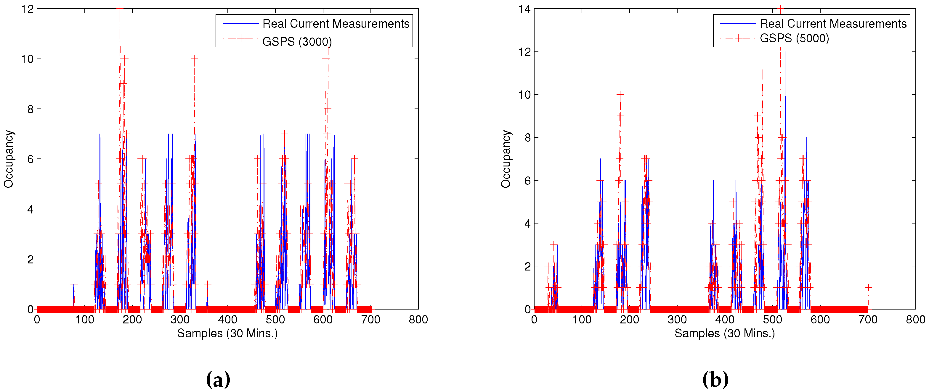
Figure 6.
Occupancy estimation using EM algorithm.
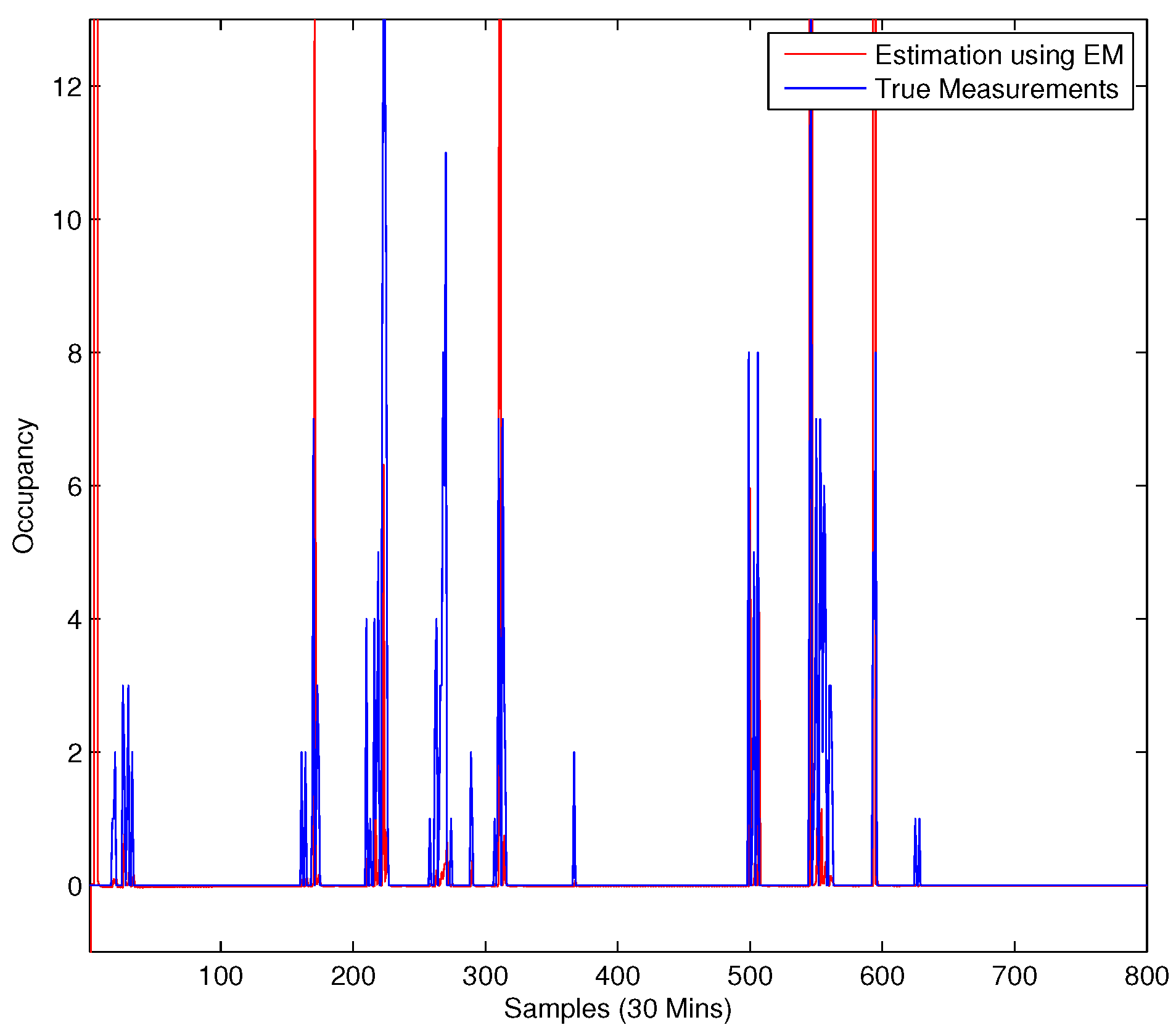
Figure 7.
Occupancy estimation using three different basis functions: (a) Gaussian basis functions; (b) Laplace basis functions; (c) Uniform basis functions.
Figure 7.
Occupancy estimation using three different basis functions: (a) Gaussian basis functions; (b) Laplace basis functions; (c) Uniform basis functions.

Figure 8.
Temperature set point for uncertain basis method.


Table 1.
Building parameter definition.
| Variables | Definition |
|---|---|
| Indoor air temperature (C) | |
| Interior-wall temperature (C) | |
| Exterior-wall core temperature (C) | |
| Cooling power () (kW) | |
| Heating power () (kW) | |
| Ambient temperature (C) | |
| Solar radiation (kW/m2) | |
| Internal heat gain (kW) |
Table 2.
Building parameter values.
| Building Parameter Values | Unit |
|---|---|
| C1 = 9.356 ×10 5 | kJ/C |
| C2 = 2.970 × 10 6 | kJ/C |
| Cw = 6.695 × 10 5 | kJ/C |
| K1 = 16.48 | kJ/C |
| K2 = 108.5 | kJ/C |
| K3 = 5 | kJ/C |
| K4 = 30.5 | kJ/C |
| K5 = 23.04 | kJ/C |
Table 3.
A sequence and mask for a system with uncertain output. Circles are input data for the function f and the square is the output data.
Table 3.
A sequence and mask for a system with uncertain output. Circles are input data for the function f and the square is the output data.
| Round | Time () | Occupancy () |
|---|---|---|
| 11 | ||
| 10 | ⓑ | |
| 9 | ⓐ | |
| 8 | ⓑ | |
| 7 | a | |
| 6 | a | |
| 5 | b | |
| 4 | a | |
| 3 | b | |
| 2 | b | |
| 1 | a |
Table 4.
Rule for the sequence and mask using a subset of 3000 points restricted to 3:00 p.m. (a-unoccupied, b-occupied).
Table 4.
Rule for the sequence and mask using a subset of 3000 points restricted to 3:00 p.m. (a-unoccupied, b-occupied).
| Input | Output | Count | Likelihood |
|---|---|---|---|
| aaa | a | 47 | 0.959 |
| b | 2 | 0.041 | |
| aab | a | 0 | 0 |
| b | 1 | 1 | |
| aba | a | 1 | 1 |
| b | 0 | 0 | |
| abb | a | 0 | 0 |
| b | 1 | 1 | |
| baa | a | 1 | 0.5 |
| b | 1 | 0.5 | |
| bab | a | 1 | 0.33 |
| b | 2 | 0.67 | |
| bba | a | 0 | 0 |
| b | 1 | 1 | |
| bbb | a | 0 | 0 |
| b | 4 | 1 |
Table 5.
Performance comparison of occupancy prediction algorithms.
| Methods | Estimation RMSE | Accuracy |
|---|---|---|
| GSPS (3000) | 3.078 | 70.0% |
| GSPS (5000) | 2.646 | 71.5% |
| EM | 3.715 | 61.5% |
| Basis-Gaussian | 3.211 | 68.4% |
| Basis-Laplace | 2.946 | 70.9% |
| Basis-Uniform | 2.571 | 72.6% |
Table 6.
Comparison of energy saving.
| Methods | Control Cost () | Energy Saving |
|---|---|---|
| Basic Control (No Occupancy info) | 5.43 | 0% |
| Basis-Gaussian (Basic Control) | 4.77 | 13% |
| Basis-Gaussian (MPC) | 4.38 | 20% |
© 2018 by the authors. Licensee MDPI, Basel, Switzerland. This article is an open access article distributed under the terms and conditions of the Creative Commons Attribution (CC BY) license (http://creativecommons.org/licenses/by/4.0/).
Share and Cite
MDPI and ACS Style
Dong, J.; Winstead, C.; Nutaro, J.; Kuruganti, T. Occupancy-Based HVAC Control with Short-Term Occupancy Prediction Algorithms for Energy-Efficient Buildings. Energies 2018, 11, 2427. https://doi.org/10.3390/en11092427
AMA Style
Dong J, Winstead C, Nutaro J, Kuruganti T. Occupancy-Based HVAC Control with Short-Term Occupancy Prediction Algorithms for Energy-Efficient Buildings. Energies. 2018; 11(9):2427. https://doi.org/10.3390/en11092427
Chicago/Turabian StyleDong, Jin, Christopher Winstead, James Nutaro, and Teja Kuruganti. 2018. "Occupancy-Based HVAC Control with Short-Term Occupancy Prediction Algorithms for Energy-Efficient Buildings" Energies 11, no. 9: 2427. https://doi.org/10.3390/en11092427
Note that from the first issue of 2016, this journal uses article numbers instead of page numbers. See further details here.