A Remedial Strategic Scheduling Model for Load Serving Entities Considering the Interaction between Grid-Level Energy Storage and Virtual Power Plants

Abstract

More renewable energy resources have been connected to the grid with the promotion of global energy strategies, which presents new opportunities for the current electricity market. However, the growing integration of renewable energy also brings more challenges, such as power system reliability and the participants’ marketable behavior. Thus, how to coordinate integrated renewable resources in the electricity market environment has gained increasing interest. In this paper, a bilevel bidding model for load serving entities (LSEs) considering grid-level energy storage (ES) and virtual power plant (VPP) is established in the day-ahead (DA) market. Then, the model is extended by considering contingencies in the intraday (ID) market. Also, according to the extended bidding model, a remedial strategic rescheduling approach for LSE’s daily profit is proposed. It provides a quantitative assessment of LSE’s loss reduction based on contingency forecasting, which can be applied to the power system dispatch to help LSEs deal with coming contingencies. Simulation results verify the correctness and effectiveness of the proposed method.

1. Introduction

More sustainable sources have been introduced into the smart grid due to the falling cost of renewable energy integration and the incentive of government energy policies [1]. However, renewable energy resources have significant uncertainties in the power output [2], which raises higher requirements on system generation reserves for reliability reasons [3,4,5]. Also, some renewable resources are small-scale and nondispatchable. They neither provide a stable power supply nor act in the electricity market as individual participants.

To address these issues, energy storage (ES) technology has attracted attention for its flexibility in power system dispatch and adjustment [6,7]. In recent years, with significant improvements in performance and cost, ES has been not only integrated into insular power networks [8], but also promoted to grid level [9]. It contributes to peak-shaving and valley-filling applications due to the rapid charging and discharging characteristics [10,11]. Simultaneously, since ES can arrive at grid level, it has more potential in the wholesale electricity market. Thus, ES owners can gain more profits by using energy arbitrage [12,13,14,15]. In addition to grid-level ES, virtual power plant (VPP) technology provides another approach to solve the issues above. In the US, VPPs can deal with the supply side, help manage demand, and ensure the reliability of grid functions through demand response (DR) and other load-shifting schemes [16,17]. Also, with a central energy management system, VPPs can coordinate the load demand and renewable energy sources [18], achieve energy trading on the wholesale electricity markets, and provide grid operators with ancillary services on behalf of small-scale and nondispatchable renewable resources [19].

The combination of grid-level ES and VPP can not only address the reliability issue of power systems with high renewable energy penetration but also help ES and VPP owners to obtain more profits in electricity market activities. However, research on smart scheduling strategies of grid-level ES and VPP is rarely done. Most of the traditional work is focused on the individual behaviors of ES/VPP and applied to energy arbitrage, operation scheduling, and demand response strategies. In [20] an ES operation and sizing approach with wind power integrated in a market environment is provided. To deal with the high wind power penetration, an ES stochastic bidding model for optimal energy and reserve on power grids is proposed in [21]. Examples of VPP behavior are studied in [22,23,24]. The research in [22,23] aims at maximizing VPP profit by incorporating demand response schemes. Multiple VPPs are considered as individual participants in the electricity market and game theory is utilized to optimize each VPP’s dispatching in [24].

Also, all the research above was done under stable operating conditions without considering the contingencies, which have a series of impacts on the scheduling of ES and VPP in the current electricity market mechanisms. Meanwhile, the interactive characteristic makes the owner’s scheduling strategy more complex under a coordinated operation environment. There is no significantly effective approach regarding coordinated scheduling considering contingencies due to the limitations of current electricity market mechanisms. In the US, most independent system operators (ISOs) implement two market mechanisms at present: the day-ahead (DA) market and the real-time (RT) market [25]. The DA market is responsible for clearing the majority of trades, while the RT market aims at balancing the power system by rescheduling the generating units. Note that when there are significant deviations of system operation in the RT market, a large number of adjustments will be brought into the rescheduling process within a short time horizon, along with heavy computational burden. Also, the adjustments may not be made economically or efficiently in the RT market [26]. The intraday (ID) market [27] is now established between the DA market and the RT market in European countries to address this issue.

While most electricity is traded in the DA market, producers and consumers can use the ID market to adjust their supply and demand commitments according to updated forecasts closer to the time of delivery [28]. With more rescheduling time, the adjustments can be made more efficiently, reducing the balancing burden in the RT market. Additionally, since some contingencies that lead to deviations of practical system operation can be predicted several hours ahead of the delivery time in the ID market, LSEs can change their bidding strategy to respond to the upcoming contingencies, reducing losses or even gaining more profits. Although the ID market is not yet established in the US, the urgency for this kind of market mechanism is sensed by ISOs [24].

In this paper, we focus on the coordinated scheduling of grid-level ES and VPP in the DA market and adjustments of ES and VPP rescheduling in the ID market through a remedial strategic bidding approach. The novelty of the paper includes: (1) a bilevel strategic bidding model considering grid-level ES and VPP established in the DA market is used; (2) by including the ID market, the strategic bidding model in the DA market is extended, considering contingencies; and (3) a remedial strategic rescheduling approach for the daily profits of LSEs is proposed to deal with forecast contingencies.

The major objective of this paper is to help LSEs reduce losses due to contingencies in the ID market. Also, hypotheses are made during the modelling process. We assume that contingencies can be predicted several hours ahead by advanced sensor technology. Meanwhile, considering model complexity and computation efficiency, the recovery cost of a specific contingency is not included in the LSE’s remedial strategic rescheduling approach. Furthermore, the bilevel strategic bidding model considering grid-level ES and VPP is the foundation of the entire remedial strategic rescheduling approach. This bilevel problem is transformed into a mixed-integer linear programming (MILP) problem, which can be effectively solved by commercial optimization software like CPLEX.

The rest of the paper is organized as follows: Section 2 formulates the strategic bidding approach for LSEs daily profit in the DA market and the remedial strategic rescheduling approach in the ID market based on a bilevel bidding model. Section 3 provides the corresponding mathematical solution to the bilevel optimization problem. Section 4 verifies the effectiveness of the proposed strategy with simulation results. Section 5 discusses the results and the hypotheses. Finally, Section 6 draws conclusions of the presented study and provides directions for future research.

2. Strategic Scheduling Model for LSEs

In this section, the entire model for the LSE’s remedial strategic scheduling is established. An overview of the implementation process is presented in Figure 1. We first formulate the grid-level ES model and VPP model in Section 2.1 and Section 2.2, respectively. Then, the bilevel LSE’s strategic scheduling model is presented in Section 2.3, with consideration of grid-level ES and VPP.

2.1. Grid-Level ES Model

The ES model is established based on its charging (or discharging) status, charging (or discharging) power, charging (or discharging) efficiency, maximum charging (or discharging) rate, self-discharging rate, and state of charge. It can be expressed as:

$$x_{i,t}+y_{i,t}=1$$

(1a)

$$0\le P_{i,t}^{ch}\le P_{i,rated}^{ch}\times x_{i,t}$$

(1b)

$$0\le P_{i,t}^{dis}\le P_{i,rated}^{dis}\times y_{i,t}$$

(1c)

$$G_{i,t}^{ch}={\eta }_i^{ch}\times P_{i,t}^{ch}\times \Delta t$$

(1d)

$$G_{i,t}^{dis}=1/{\eta }_i^{dis}\times P_{i,t}^{dis}\times \Delta t$$

(1e)

$$G_{i,t}^{ch}\le G_{i,cont}^{ch}$$

(1f)

$$G_{i,t}^{dis}\le G_{i,cont}^{dis}$$

(1g)

$$E_{i,t}^{self}=E_{i,t-1}^{stored}\times (1-r_i)$$

(1h)

$$E_{i,1}^{stored}=E_{i,init}^{stored}-E_{i,1}^{self}+G_{i,1}^{ch}-G_{i,1}^{dis}$$

(1i)

$$E_{i,t}^{stored}=E_{i,t-1}^{stored}-E_{i,t}^{self}+G_{i,t}^{ch}-G_{i,t}^{dis}$$

(1j)

$$SO{C}_{i,\min }\le E_{i,t}^{stored}/E_{i,\max }\le SO{C}_{i,\max }$$

(1k)

Constraint (1a) requires that the status of ES must be either charging or discharging at a particular period t. Constraints (1b) and (1c) ensure that the ES’s charging or discharging power in period t is limited by the charging or discharging status and the maximum rates. Constraints (1d) and (1e) represent the charging or discharging capacity of ES considering the efficiency in period t; $\Delta t$ in (1d) and (1e) is equal to 1 h. Constraints (1f) and (1g) require that the charging/discharging capacity must be less than the upper charging/discharging capacity due to the contract with the ISO. Constraint (1h) represents the self-discharging energy in period t. Constraints (1i) and (1j) represent the stored energy at the end of each period. Constraint (1k) imposes the maximum and minimum state of charge constraints for ES.

2.2. Interruptible Load-Based Demand Response Virtual Power Plant Model

A virtual power plant is a system in which different types of small-scale power generation sources, such as wind turbines, small hydro, photovoltaics, natural gas-fired reciprocating engines, and micro combined heat and power systems, are integrated. With a central authority, a VPP integrating a cluster of dispatchable and nondispatchable sources can not only provide a reliable power supply but also participate in the wholesale electricity market.

We modelled the VPP by DR resources. An interruptible load-based DR (IBDR) is chosen in this paper. According to the responding mechanism, DR programs are usually classified into two main categories: price-based and incentive-based. The IBDR above is an incentive-based DR. In the price-based DR mechanism, customers can obtain the provided rebates by willingly reducing their power demand. In contrast, in the incentive-based DR mechanism, customers can get compensated for their passive electricity interruptions. Therefore, the incentive-based DR provides a more convenient way of timely dispatching in power systems.

We assume that by signing a contract with IBDR customers, LSEs can shed the load at the compensatory price ${\beta }_{i,t}$ for no longer than the maximum response time $T_{up,i}^{\max }$. Also, the contract requires that the period between two adjacent interruptions must be no less than the minimum time interval $T_{down,i}^{\min }$. Thus, constraints on the status of IBDR-VPP can be expressed as follows:

$${\displaystyle \sum _{t=1}^{T_i^{off}}{v}_{i,t}=0}$$

(2a)

$${\displaystyle \sum _{t=k}^{k+T_{down,i}^{\min }-1}(1-v_{i,t})\ge T_{down,i}^{\min }}(v_{i,k-1}-v_{i,k}),\forall k=T_i^{off}+1,\cdots ,T^{\mathsf{\Omega }}-T_{down,i}^{\min }+1$$

(2b)

$${\displaystyle \sum _{t=k}^{T^{\mathsf{\Omega }}}[1-v_{i,t}-(v_{i,k-1}-v_{i,k})]\ge 0},\forall k=T^{\mathsf{\Omega }}-T_{down,i}^{\min }+1,\cdots ,T^{\mathsf{\Omega }}$$

(2c)

$$\left({\displaystyle \sum _{t=k}^{k+T_{up,i}^{\max }}{v}_{i,t}}\right)\le T_{up,i}^{\max },\forall k=T_i^{off}+1,\cdots ,T^{\mathsf{\Omega }}-T_{up,i}^{\max }$$

(2d)

$$\forall T^{\mathsf{\Omega }}\in \{T^N,T^P,T^O\}$$

(2e)

Constraint (2a) sets the initial status of the VPP according to the previous operations. Constraint (2b) ensures that the VPP stays offline for at least $T_{down}^{\min }$ consecutive hours once it shuts down. Constraint (2c), as a complement to (2b), further ensures that the VPP stays offline until the end of the period in question if the rest hours are less than $T_{down}^{\min }$. Constraint (2d) requires that the VPP must not stay online for more than $T_{up}^{\max }$ consecutive hours.

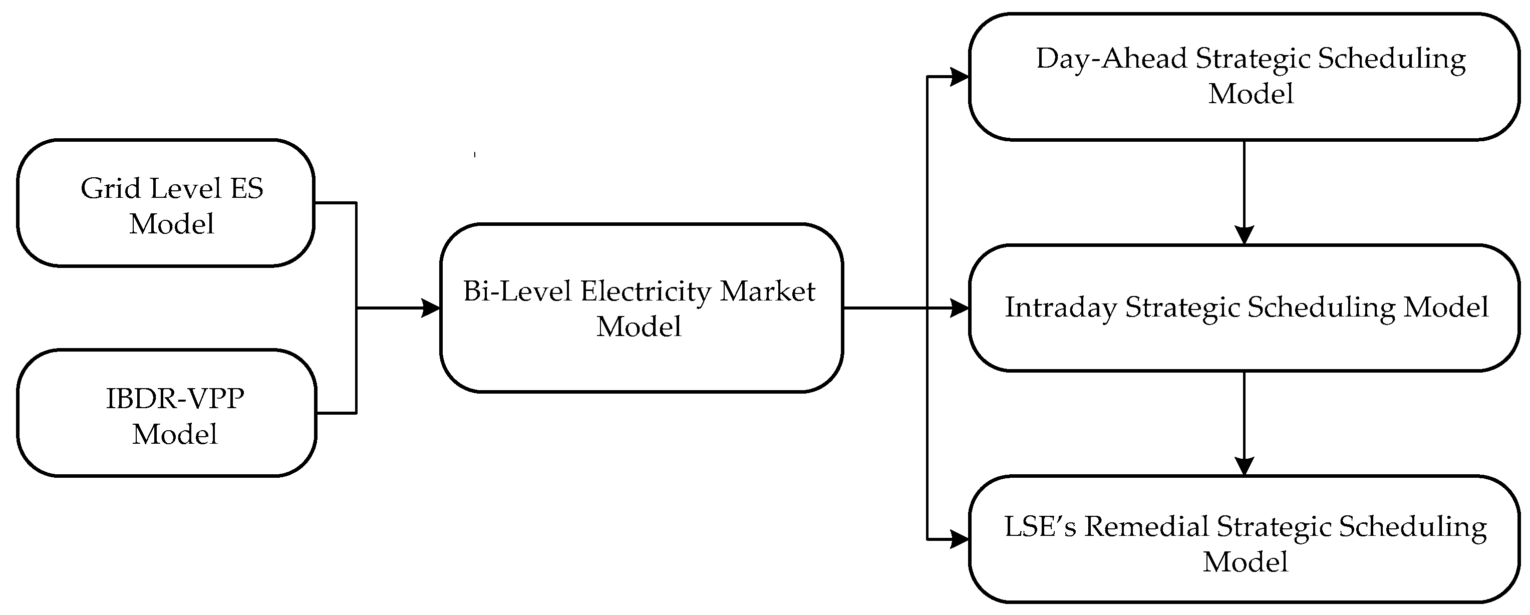
2.3. Bilevel Electricity Market Models

In this section, the day-ahead/intraday and remedial strategic scheduling approaches for LSEs are based on the bilevel strategic model, in which the upper level represents the process of the LSE’s profit maximization and the lower level simulates the process of the ISO’s market clearing.

2.3.1. Day-Ahead Strategic Scheduling Model

We assume that the grid-level ES and IBDR-VPP have comparable capacities as conventional power plants. In other words, they are participators rather than price-takers in the electricity market environment. They are able to make both price and quantity bids in the electricity market.

Thus, from the perspective of an LSE owning grid-level ESs and IBDR-VPPs, the optimization objective is formulated as:

$$\max {\displaystyle \sum _{t=1}^T{\displaystyle \sum _{i=1}^N\left({\pi }_{i,t,DA}(G_{i,t,DA}^V+G_{i,t,DA}^{dis})-{\beta }_{i,t}{G}_{i,t,DA}^V-{\gamma }_{i,t}{G}_{i,t,DA}^{ch}\right)}}$$

(3a)

subject to:

grid-level ES constraints in (1a)–(1k)

(3b)

IBDR-VPP constraints in (2a)–(2e)

(3c)

$$\left\{{\pi }_{i,t,DA},G_{i,t,DA}^V,G_{i,t,DA}^{dis}\right\}\in \arg \{\min {\displaystyle \sum _{t=1}^T{\displaystyle \sum _{i=1}^N\left({\alpha }_{i,t,DA}^V{G}_{i,t,DA}^V+{\alpha }_{i,t,DA}^{dis}{G}_{i,t,DA}^{dis}+{\alpha }_{i,t,DA}^C{G}_{i,t,DA}^C\right)}}$$

(3d)

$${\displaystyle \sum _i\left(G_{i,t,DA}^V+G_{i,t,DA}^{dis}+G_{i,t,DA}^C\right)}={\displaystyle \sum _i\left(D_{i,t}+G_{i,t,DA}^{ch}\right)}:{\lambda }_{t,DA},\forall t$$

(3e)

$$\{\begin{array}{l}{G}_{i,\min }^V\le G_{i,t,DA}^V\le G_{i,\max }^V:{\omega }_{i,t,DA}^{V\_\min },{\omega }_{i,t,DA}^{V\_\max },\forall i\forall t\\ G_{i,\min }^{dis}\le G_{i,t,DA}^{dis}\le G_{i,\max }^{dis}:{\omega }_{i,t,DA}^{dis\_\min },{\omega }_{i,t,DA}^{dis\_\max },\forall i\forall t\\ G_{i,\min }^C\le G_{i,t,DA}^C\le G_{i,\max }^C:{\omega }_{i,t,DA}^{C\_\min },{\omega }_{i,t,DA}^{C\_\max },\forall i\forall t\end{array}$$

(3f)

$$-Limi{t}_l\le {\displaystyle \sum _{i}GS{F}_{l,i}\times (G_{i,t,DA}^V+G_{i,t,DA}^{dis}+G_{i,t,DA}^C-G_{i,t,DA}^{ch}-D_{i,t})}\le Limi{t}_l:{\mu }_{l,t,DA}^{\min },{\mu }_{l,t,DA}^{\max },\forall t\forall l\}$$

(3g)

$$\begin{array}{l}\psi =\left({\displaystyle \sum _{i,t}{\alpha }_{i,t,DA}^V{G}_{i,t,DA}^V+}{\alpha }_{i,t,DA}^{dis}{G}_{i,t,DA}^{dis}+{\alpha }_{i,t,DA}^C{G}_{i,t,DA}^C\right)-{\displaystyle \sum _i{\lambda }_{t,DA}}\left({\displaystyle \sum _i\left(G_{i,t,DA}^V+G_{i,t,DA}^{dis}+G_{i,t,DA}^C\right)}-{\displaystyle \sum _i{D}_{i,t}}\right)\\ -{\displaystyle \sum _{l,t}{\mu }_{l,t,DA}^{\min }}\left({\displaystyle \sum _{i}GS{F}_{l,i}\times (G_{i,t,DA}^V+G_{i,t,DA}^{dis}+G_{i,t,DA}^C-D_{i,t})}-Limi{t}_l\right)\\ -{\displaystyle \sum _{l,t}{\mu }_{l,t,DA}^{\max }}\left(Limi{t}_l-{\displaystyle \sum _{i}GS{F}_{l,i}\times (G_{i,t,DA}^V+G_{i,t,DA}^{dis}+G_{i,t,DA}^C-D_{i,t})}\right)\\ -{\displaystyle \sum _{i,t}{\omega }_{i,t,DA}^{V\_\min }}\left(G_{i,t,DA}^V-G_{i,\min }^V\right)-{\displaystyle \sum _{i,t}{\omega }_{i,t,DA}^{V\_\max }}\left(G_{i,\max }^V-G_{i,t,DA}^V\right)\\ -{\displaystyle \sum _{i,t}{\omega }_{i,t,DA}^{dis\_\min }}\left(G_{i,t,DA}^{dis}-G_{i,\min }^{dis}\right)-{\displaystyle \sum _{i,t}{\omega }_{i,t,DA}^{dis\_\max }}\left(G_{i,\max }^{dis}-G_{i,t,DA}^{dis}\right)\\ -{\displaystyle \sum _{i,t}{\omega }_{i,t,DA}^{C\_\min }}\left(G_{i,t,DA}^C-G_{i,\min }^C\right)-{\displaystyle \sum _{i,t}{\omega }_{i,t,DA}^{C\_\max }}\left(G_{i,\max }^C-G_{i,t,DA}^C\right)\end{array}$$

(3h)

$${\pi }_{i,t,DA}=\frac{\partial \psi }{\partial D_{i,t}}={\lambda }_{t,DA}+{\displaystyle \sum _{i}GS{F}_{l,i}\times ({\mu }_{l,t,DA}^{\min }-{\mu }_{l,t,DA}^{\max })}$$

(3i)

The objective function of the upper level expressed in constraint (3a) aims to maximize the LSE’s daily profit, and the objective function of lower level in constraint (3d) is the process of market clearing, which is managed by an ISO. In this model, the ISO can minimize the total cost of electricity purchased from conventional generators, grid-level ESs, and virtual generators. Constraint (3e) represents the power-balancing constraint for each time interval. Constraint (3f) ensures that the outputs of conventional generators, ESs, and virtual generators are limited by each other’s maximum and minimum outputs. Constraint (3g) requires that the bidirectional power of each transmission line must be less than the transmission line power rate. Constraint (3h) is the Lagrangian function based on (3d)–(3g), and the LMP ${\pi }_{i,t,s}$ can be calculated according to (3h)–(3i).

2.3.2. Intraday Strategic Scheduling Model

It is feasible that if there is no deviation in price and quantity bids, the power system scheduling in the ID market will be the same as that in the DA market. Nevertheless, there are many factors, such as contingencies and weather variations, in the ID market. Thus, the ID market scheduling should be recalculated according to the actual grid operation status. Hence, the ID market can be viewed as a complementary part of the DA market, although the ID market is closer to the time of delivery.

In this section, we aim to quantify the impact of contingencies on ID market rescheduling and LSE’s daily profit. Virtual generators, ESs, and conventional generators are assumed to participate in the ID market rescheduling process with the rest of their capacity. Meanwhile, we assume that the contingencies in question consist of ES outage and IBDR-VPP outage. Note that although this paper only proposes an ES/IBDR-VPP outage model, similar modeling methods such as deficiency of DR can also be taken into consideration with regard to contingency.

The DA market bidding process is considered as an input to the ID market optimization, and a scenario (denoted by $s^{\ast }$) with a specific contingency is realized. Then, the optimization problem of LSE’s daily profit can be expressed as:

$$\max {\displaystyle \sum _{t=1}^T{\displaystyle \sum _{i=1}^N{f}_{DA}(i,t,s^{\ast })}}+{\displaystyle \sum _{t=t_O}^T\left({\displaystyle \sum _{i=1}^N{\pi }_{i,t,ID}(G_{i,t,ID}^V+G_{i,t,ID}^{dis})}-{\displaystyle \sum _{i=1}^N{\beta }_{i,t}{G}_{i,t,ID}^V-}{\displaystyle \sum _{i=1}^N{\gamma }_{i,t}{G}_{i,t,ID}^{ch}}\right)}$$

(4a)

subject to:

updated grid-level ES constraints in (1a)–(1e)

(4b)

$$G_{i,t,ID}^{ch}\le G_{i,cont}^{ch}-{\overline{G}}_{i,t,DA}^{ch}$$

(4c)

$$G_{i,t,ID}^{dis}\le G_{i,cont}^{dis}-{\overline{G}}_{i,t,DA}^{dis}$$

(4d)

$$E_{i,t,s\ast }^{stored}={\overline{E}}_{i,t,DA}^{stored}+G_{i,t,ID}^{ch}-G_{i,t,ID}^{dis}$$

(4e)

$$SO{C}_{i,\min }\le E_{i,t,s\ast }^{stored}/E_{i,\max }\le SO{C}_{i,\max }$$

(4f)

updated IBDR-VPP constraints:

$${\displaystyle \sum _{t=1}^{T_{i,s\ast }^{off}}{v}_{i,t}=0}$$

(4g)

$${\displaystyle \sum _{t=k}^{k+T_{down,i}^{\min }-1}(1-v_{i,t})\ge T_{down,i}^{\min }}(v_{i,k-1}-v_{i,k}),\forall k=T_{i,s\ast }^{off}+1,\cdots ,T^{\mathsf{\Omega }}-T_{down,i}^{\min }+1$$

(4h)

constraints in (2c)–(2e)

(4i)

$$\{{\pi }_{i,t,ID},G_{i,t,ID}^V,G_{i,t,ID}^{dis}\}\in \arg \{\min {\displaystyle \sum _{i,t}{\alpha }_{i,t,ID}^V{G}_{i,t,ID}^V+}{\alpha }_{i,t,ID}^{dis}{G}_{i,t,ID}^{dis}+{\alpha }_{i,t,ID}^C{G}_{i,t,ID}^C$$

(4j)

$${\displaystyle \sum _i\left(G_{i,t,ID}^V+G_{i,t,ID}^{dis}+G_{i,t,ID}^C+{\overline{G}}_{i,t,DA}^V+{\overline{G}}_{i,t,DA}^{dis}+{\overline{G}}_{i,t,DA}^C\right)}={\displaystyle \sum _i\left(D_{i,t}+G_{i,t,ID}^{dis}+{\overline{G}}_{i,t,DA}^{dis}\right)}:{\lambda }_{t,ID},\forall t$$

(4k)

$$\{\begin{array}{l}{G}_{i,\min }^V-{\overline{G}}_{i,t,DA}^V\le G_{i,t,ID}^V\le G_{i,\max }^V-{\overline{G}}_{i,t,DA}^V:{\omega }_{i,t,ID}^{V\_\min },{\omega }_{i,t,ID}^{V\_\max },\forall i\forall t\\ G_{i,\min }^{dis}-{\overline{G}}_{i,t,DA}^{dis}\le G_{i,t,ID}^{dis}\le G_{i,\max }^{dis}-{\overline{G}}_{i,t,DA}^{dis}:{\omega }_{i,t,ID}^{dis\_\min },{\omega }_{i,t,ID}^{dis\_\max },\forall i\forall t\\ G_{i,\min }^C-{\overline{G}}_{i,t,DA}^C\le G_{i,t,ID}^C\le G_{i,\max }^C-{\overline{G}}_{i,t,DA}^C:{\omega }_{i,t,ID}^{C\_\min },{\omega }_{i,t,ID}^{C\_\max },\forall i\forall t\end{array}$$

(4l)

$$\begin{array}{c}-Limi{t}_l\le {\displaystyle \sum _{i}GS{F}_{l,i}\times (G_{i,t,ID}^V+G_{i,t,ID}^{dis}+G_{i,t,ID}^C+{\overline{G}}_{i,t,DA}^V+{\overline{G}}_{i,t,DA}^{dis}+{\overline{G}}_{i,t,DA}^C-G_{i,t,ID}^{ch}-{\overline{G}}_{i,t,DA}^{ch}-D_{i,t})}\\ \le Limi{t}_l:{\mu }_{l,t,ID}^{\min },{\mu }_{l,t,ID}^{\max },\forall t\forall l\}\end{array}$$

(4m)

$${\pi }_{i,t,ID}={\lambda }_{t,ID}+{\displaystyle \sum _{i}GS{F}_{l,i}\times ({\mu }_{l,t,ID}^{\min }-{\mu }_{l,t,ID}^{\max })}$$

(4n)

Similar to the bilevel day-ahead strategic scheduling model in the previous section, the upper-level objective function expressed in (4a) is to maximize the LSE’s daily profit. Note that ${\displaystyle \sum _{i,t}{f}_{DA}(i,t,s^{\ast })}$ is a constant representing the LSE’s profit in the DA market. For completeness, it is added in (4a). The lower-level objective function in (4j) simulates the process of market clearing. In (4c)–(4f), constraints for the ES’s charging/discharging capacity, stored energy, and state of charge constraints are updated. In addition, (4g) and (4h) represent the updated constraints for the IBDR-VPP’s status. Constraints (4k)–(4m) for power balancing, virtual generators, ES and conventional generator output limits, and transmission line power limit are also updated to accommodate the ID market rescheduling process.

2.3.3. LSE’s Remedial Strategic Scheduling Model

There is neither enough time nor adequate capacity for the LSE’s generating units (including virtual generators, ESs) to reschedule after its inner contingency. In other words, the electricity deficiency due to ES/IBDR-VPP outage may not be compensated only by rescheduling the other ESs or IBDR-VPPs in good condition. Then, the conventional generators belonging to other LSEs will participate in the rescheduling process with the rest of their capacity. From the perspective of daily profit, if an LSE have more time to reschedule all of its units before a specific contingency occurs, the loss will be further reduced.

We assume that a contingency can be predicted several hours ahead by advanced sensor technology. Thus, during the contingency anticipation time, the LSE can reduce the loss due to the contingency by rescheduling not only the good generator units but also the unit that will have an outage several hours later. This remedial strategic scheduling model can be established based on the intraday strategic scheduling model in Section 2.2. With some modifications to (4a), the new optimization problem is expressed as:

$$\max {\displaystyle \sum _{t=1}^T{\displaystyle \sum _{i=1}^N{f}_{DA}(i,t,s^{\ast })}}+{\displaystyle \sum _{t=t_P}^{t_O}{\displaystyle \sum _{i=1}^N{f}_{ID,P}(i,t,s^{\ast })}}+{\displaystyle \sum _{t=t_O}^T{\displaystyle \sum _{i=1}^N{f}_{ID,O}(i,t,s^{\ast })}}$$

(5a)

subject to:

$${\displaystyle \sum _{i=1}^N{f}_{ID,\varphi }(i,t,s^{\ast })=}{\displaystyle \sum _{i=1}^N{\pi }_{i,t,ID}(G_{i,t,ID}^V+G_{i,t,ID}^{dis})}-{\displaystyle \sum _{i=1}^N{\beta }_{i,t}{G}_{i,t,ID}^V-}{\displaystyle \sum _{i=1}^N{\gamma }_{i,t}{G}_{i,t,ID}^{ch}},\forall \varphi \in \{P,O\}$$

(5b)

constraints in (4b)–(4n)

(5c)

3. Mathematical Solutions

The bilevel strategic model is the basis of the LSE’s strategic scheduling approach in both the DA and ID markets. Also, except for the differences between the bidding capacities of generating units in the DA and ID markets, the main mathematical formulation steps are similar. The general solution processes for the bilevel mode are presented in the following subsections.

3.1. Formulation of a Mathematic Program with Equilibrium Constraints (MPEC)

$$\max {\displaystyle \sum _{i,t}\left({\pi }_{i,t,\psi }(G_{i,t,\psi }^V+G_{i,t,\psi }^{dis})-{\beta }_{i,t}{G}_{i,t,\psi }^V-{\gamma }_{i,t}{G}_{i,t,\psi }^{ch}\right)}$$

(6a)

subject to:

constraints in (3b) and (3c)

(6b)

$$\{\begin{array}{l}{\alpha }_{i,t,\psi }^V={\lambda }_{t,\psi }+\left({\omega }_{i,t,\psi }^{V\_\min }-{\omega }_{i,t,\psi }^{V\_\max }\right)+{\displaystyle \sum _{i}GS{F}_{l,i}\times ({\mu }_{l,t,\psi }^{\min }-{\mu }_{l,t,\psi }^{\max })}\\ {\alpha }_{i,t,\psi }^{dis}={\lambda }_{t,\psi }+\left({\omega }_{i,t,\psi }^{dis\_\min }-{\omega }_{i,t,\psi }^{dis\_\max }\right)+{\displaystyle \sum _{i}GS{F}_{l,i}\times ({\mu }_{l,t,\psi }^{\min }-{\mu }_{l,t,\psi }^{\max })}\end{array}$$

(6c)

$$\{\begin{array}{l}0\le {\omega }_{i,t,\psi }^{V\_\min }\perp \left(G_{i,t,\psi }^V-G_{i,\min }^V\right)\ge 0,\forall i\forall t\\ 0\le {\omega }_{i,t,\psi }^{V\_\max }\perp \left(G_{i,\max }^V-G_{i,t,\psi }^V\right)\ge 0,\forall i\forall t\end{array}$$

(6d)

$$\{\begin{array}{l}0\le {\omega }_{i,t,\psi }^{dis\_\min }\perp \left(G_{i,t,\psi }^{dis}-G_{i,\min }^{dis}\right)\ge 0,\forall i\forall t\\ 0\le {\omega }_{i,t,\psi }^{dis\_\max }\perp \left(G_{i,\max }^{dis}-G_{i,t,\psi }^{dis}\right)\ge 0,\forall i\forall t\end{array}$$

(6e)

$$\{\begin{array}{l}0\le {\omega }_{i,t,\psi }^{C\_\min }\perp \left(G_{i,t,\psi }^C-G_{i,\min }^C\right)\ge 0,\forall i\forall t\\ 0\le {\omega }_{i,t,\psi }^{C\_\max }\perp \left(G_{i,\max }^C-G_{i,t,\psi }^C\right)\ge 0,\forall i\forall t\end{array}$$

(6f)

$$\{\begin{array}{l}0\le {\mu }_{l,t,\psi }^{\min }\perp {\displaystyle \sum _{i}GS{F}_{l,i}\times (G_{i,t,\psi }^V+G_{i,t,\psi }^{dis}+G_{i,t,\psi }^C-G_{i,t,\psi }^{ch}-D_{i,t})}-Limi{t}_l\ge 0,\forall i\forall t\\ 0\le {\mu }_{l,t,\psi }^{\max }\perp Limi{t}_l-{\displaystyle \sum _{i}GS{F}_{l,i}\times (G_{i,t,\psi }^V+G_{i,t,\psi }^{dis}+G_{i,t,\psi }^C-G_{i,t,\psi }^{ch}-D_{i,t})}\ge 0,\forall i\forall t\end{array}$$

(6g)

$$\forall \psi \in \left\{DA,ID\right\}$$

(6h)

The bilevel optimization problem is transformed into an MPEC integrating the lower-level problem with Karush–Kuhn–Tucker (KKT) conditions as extra complementarity constraints in (6c)–(6g).

3.2. Mixed-Integer Linear Programming (MILP) Solution

To formulate an MILP problem, the nonlinearities must be eliminated. The model expressed in (6a)–(6g) is nonlinear because of ${\pi }_{i,t,\psi }(G_{i,t,\psi }^V+G_{i,t,\psi }^{dis})$ in (6a) and a series of complementarity constraints in (6c)–(6g). The objective function of the primary problem is equal to that of the corresponding dual problem according to the strong duality theory. Thus, the lower-level objective in (3d) at each period can be expressed as:

$$\begin{array}{ll}\sum _i\left({\alpha }_{i,\psi }^V{G}_{i,\psi }^V+{\alpha }_{i,\psi }^{dis}{G}_{i,\psi }^{dis}+{\alpha }_{i,\psi }^C{G}_{i,\psi }^C\right)=& {\lambda }_{\psi }{\displaystyle \sum _i{D}_i}-{\displaystyle \sum _i{\omega }_{i,\psi }^{V\_\max }{G}_{i,\max }^V}+{\displaystyle \sum _i{\omega }_{i,\psi }^{V\_\min }{G}_{i,\min }^V}-{\displaystyle \sum _i{\omega }_{i,\psi }^{dis\_\max }{G}_{i,\max }^{dis}}\\ & +{\displaystyle \sum _i{\omega }_{i,\psi }^{dis\_\min }{G}_{i,\min }^{dis}}-{\displaystyle \sum _i{\omega }_{i,\psi }^{C\_\max }{G}_{i,\max }^C}+{\displaystyle \sum _i{\omega }_{i,\psi }^{C\_\min }{G}_{i,\min }^C}\\ & +{\displaystyle \sum _l{\mu }_{l,\psi }^{\min }\left({\displaystyle \sum _{i}GS{F}_{l,i}\times D_i}-Limi{t}_l\right)}\\ & -{\displaystyle \sum _l{\mu }_{l,\psi }^{\min }\left({\displaystyle \sum _{i}GS{F}_{l,i}\times D_i}+Limi{t}_l\right)}\end{array}$$

(7a)

Also, based on constraints (6d)–(6f), Equations (7b)–(7d) are obtained:

$$\{\begin{array}{l}{\omega }_{i,\psi }^{V\_\min }{G}_{i,\psi }^V={\omega }_{i,\psi }^{V\_\min }{G}_{i,\min }^V\\ {\omega }_{i,\psi }^{V\_\max }{G}_{i,\psi }^V={\omega }_{i,\psi }^{V\_\max }{G}_{i,\max }^V\end{array}$$

(7b)

$$\{\begin{array}{l}{\omega }_{i,\psi }^{dis\_\min }{G}_{i,\psi }^{dis}={\omega }_{i,\psi }^{dis\_\min }{G}_{i,\min }^{dis}\\ {\omega }_{i,\psi }^{dis\_\max }{G}_{i,\psi }^{dis}={\omega }_{i,\psi }^{dis\_\max }{G}_{i,\max }^{dis}\end{array}$$

(7c)

$$\{\begin{array}{l}{\omega }_{i,\psi }^{C\_\min }{G}_{i,\psi }^C={\omega }_{i,\psi }^{C\_\min }{G}_{i,\min }^C\\ {\omega }_{i,\psi }^{C\_\max }{G}_{i,\psi }^C={\omega }_{i,\psi }^{C\_\max }{G}_{i,\max }^C\end{array}$$

(7d)

Then, the nonlinear product term ${\pi }_{i,t,\psi }(G_{i,t,\psi }^V+G_{i,t,\psi }^{dis})$ can be rewritten with (3i), (6c), and (7b)–(7d):

$$\begin{gathered} \sum _i{\pi }_{i,\psi }(G_{i,\psi }^V+G_{i,\psi }^{dis})={\displaystyle \sum _i({\alpha }_{i,\psi }^V{G}_{i,\psi }^V+{\alpha }_{i,\psi }^{dis}{G}_{i,\psi }^{dis})}-{\displaystyle \sum _i\left(\left({\omega }_{i,\psi }^{V\_\min }-{\omega }_{i,\psi }^{V\_\max }\right)G_{i,\psi }^V+\left({\omega }_{i,\psi }^{V\_\min }-{\omega }_{i,\psi }^{V\_\max }\right)G_{i,\psi }^V\right)} \\ ={\displaystyle \sum _i({\alpha }_{i,\psi }^V{G}_{i,\psi }^V+{\alpha }_{i,\psi }^{dis}{G}_{i,\psi }^{dis})}-{\displaystyle \sum _i\left({\omega }_{i,\psi }^{V\_\min }{G}_{i,min}^V-{\omega }_{i,\psi }^{V\_\max }{G}_{i,max}^V\right)} \\ -{\displaystyle \sum _i\left({\omega }_{i,\psi }^{dis\_\min }{G}_{i,min}^{dis}-{\omega }_{i,\psi }^{dis\_\max }{G}_{i,max}^{dis}\right)} \end{gathered}$$

(7e)

Substituting (7a) into (7e), Equation (7f) can be obtained:

$$\begin{array}{c}{\displaystyle \sum _{i=1}^N{\pi }_{i,\psi }(G_{i,\psi }^V+G_{i,\psi }^{dis})}={\lambda }_{\psi }{\displaystyle \sum _{i=1}^N{D}_i}-{\displaystyle \sum _{i=1}^N{\omega }_{i,\psi }^{C\_\max }{G}_{i,\max }^C}+{\displaystyle \sum _{i=1}^N{\omega }_{i,\psi }^{C\_\min }{G}_{i,\min }^C+{\displaystyle \sum _{l=1}^M{\mu }_{l,\psi }^{\min }\left({\displaystyle \sum _{i=1}^{N}GS{F}_{l,i}\times D_i}-Limi{t}_l\right)}}\\ -{\displaystyle \sum _{l=1}^M{\mu }_{l,\psi }^{\min }\left({\displaystyle \sum _{i=1}^{N}GS{F}_{l,i}\times D_i}+Limi{t}_l\right)}-{\displaystyle \sum _{i=1}^N{\alpha }_{i,\psi }^C{G}_{i,\psi }^C}\end{array}$$

(7f)

Finally, the MILP problem that is converted from the MPEC in (6a)–(6f) can be expressed as:

$$\begin{array}{l}\max {\displaystyle \sum _{i,t}\left({\pi }_{i,t,\psi }(G_{i,t,\psi }^V+G_{i,t,\psi }^{dis})-{\beta }_{i,t}{G}_{i,t,\psi }^V-{\gamma }_{i,t}{G}_{i,t,\psi }^{ch}\right)}\\ ={\displaystyle \sum _t[{\lambda }_{t,\psi }{\displaystyle \sum _i{D}_{i,t}}-{\displaystyle \sum _i{\omega }_{i,t,\psi }^{C\_\max }{G}_{i,t,\max }^C}+{\displaystyle \sum _i{\omega }_{i,t,\psi }^{C\_\min }{G}_{i,t,\min }^C}+{\displaystyle \sum _l{\mu }_{l,t,\psi }^{\min }\left({\displaystyle \sum _{i=1}^{N}GS{F}_{l,i}\times D_{i,t}}-Limi{t}_l\right)}}\\ -{\displaystyle \sum _l{\mu }_{l,t,\psi }^{\min }\left({\displaystyle \sum _{i=1}^{N}GS{F}_{l,i}\times D_{i,t}}+Limi{t}_l\right)}-{\displaystyle \sum _i{\alpha }_{i,t,\psi }^C{G}_{i,t,\psi }^C}-{\displaystyle \sum _i{\beta }_{i,t}{G}_{i,t,\psi }^V}-{\displaystyle \sum _i{\gamma }_{i,t}{G}_{i,t,\psi }^{ch}}]\end{array}$$

(8a)

subject to:

constraints in (6b) and (6c)

(8b)

$$\{\begin{array}{l}0\le G_{i,t,\psi }^V-G_{i,\min }^V\le Big{M}_{\omega }^{V\_\min }{\nu }_{\omega ,i,t}^{V\_\min },\forall i\forall t\\ 0\le {\omega }_{i,t,\psi }^{V\_\min }\le Big{M}_{\omega }^{V\_\min }\left(1-{\nu }_{\omega ,i,t}^{V\_\min }\right),\forall i\forall t\\ 0\le G_{i,\max }^V-G_{i,t,\psi }^V\le Big{M}_{\omega }^{V\_\max }{\nu }_{\omega ,i,t}^{V\_\max },\forall i\forall t\\ 0\le {\omega }_{i,t,\psi }^{V\_\max }\le Big{M}_{\omega }^{V\_\max }\left(1-{\nu }_{\omega ,i,t}^{V\_\max }\right),\forall i\forall t\end{array}$$

(8c)

$$\{\begin{array}{l}0\le G_{i,t,\psi }^{dis}-G_{i,\min }^{dis}\le Big{M}_{\omega }^{dis\_\min }{\nu }_{\omega ,i,t}^{dis\_\min },\forall i\forall t\\ 0\le {\omega }_{i,t,\psi }^{dis\_\min }\le Big{M}_{\omega }^{dis\_\min }\left(1-{\nu }_{\omega ,i,t}^{dis\_\min }\right),\forall i\forall t\\ 0\le G_{i,\max }^{dis}-G_{i,t,\psi }^{dis}\le Big{M}_{\omega }^{dis\_\max }{\nu }_{\omega ,i,t}^{dis\_\max },\forall i\forall t\\ 0\le {\omega }_{i,t,\psi }^{dis\_\max }\le Big{M}_{\omega }^{dis\_\max }\left(1-{\nu }_{\omega ,i,t}^{dis\_\max }\right),\forall i\forall t\end{array}$$

(8d)

$$\{\begin{array}{l}0\le G_{i,t,\psi }^C-G_{i,\min }^C\le Big{M}_{\omega }^{C\_\min }{\nu }_{\omega ,i,t}^{C\_\min },\forall i\forall t\\ 0\le {\omega }_{i,t,\psi }^{C\_\min }\le Big{M}_{\omega }^{C\_\min }\left(1-{\nu }_{\omega ,i,t}^{C\_\min }\right),\forall i\forall t\\ 0\le G_{i,\max }^C-G_{i,t,\psi }^C\le Big{M}_{\omega }^{C\_\max }{\nu }_{\omega ,i,t}^{C\_\max },\forall i\forall t\\ 0\le {\omega }_{i,t,\psi }^{C\_\max }\le Big{M}_{\omega }^{C\_\max }\left(1-{\nu }_{\omega ,i,t}^{C\_\max }\right),\forall i\forall t\end{array}$$

(8e)

$$\{\begin{array}{l}0\le Limi{t}_l+{\displaystyle \sum _{i}GS{F}_{l,i}\times (G_{i,t,\psi }^V+G_{i,t,\psi }^{dis}+G_{i,t,\psi }^C-G_{i,t,\psi }^{ch}-D_{i,t})}\le Big{M}_{\mu }^{\min }{\nu }_{\mu ,l,t}^{\min },\forall l\forall t\\ 0\le {\mu }_{l,t,\psi }^{\min }\le Big{M}_{\mu }^{\min }\left(1-{\nu }_{\omega ,l,t}^{\min }\right),\forall l\forall t\\ 0\le Limi{t}_l-{\displaystyle \sum _{i}GS{F}_{l,i}\times (G_{i,t,\psi }^V+G_{i,t,\psi }^{dis}+G_{i,t,\psi }^C-G_{i,t,\psi }^{ch}-D_{i,t})}\le Big{M}_{\mu }^{\max }{\nu }_{\mu ,l,t}^{\min },\forall l\forall t\\ 0\le {\mu }_{l,t,\psi }^{\max }\le Big{M}_{\mu }^{\max }\left(1-{\nu }_{\omega ,l,t}^{\max }\right),\forall l\forall t\end{array}$$

(8f)

where $Big{M}_{\omega }^{V\_\min }$, $Big{M}_{\omega }^{V\_\max }$, $Big{M}_{\omega }^{dis\_\min }$, $Big{M}_{\omega }^{dis\_\max }$, $Big{M}_{\omega }^{C\_\min }$, $Big{M}_{\omega }^{C\_\max }$, $Big{M}_{\mu }^{\min }$, and $Big{M}_{\mu }^{\max }$ are big constants, and ${\nu }_{\omega ,i,t}^{V\_\min }$, ${\nu }_{\omega ,i,t}^{V\_\max }$, ${\nu }_{\omega ,i,t}^{dis\_\min }$, ${\nu }_{\omega ,i,t}^{dis\_\max }$, ${\nu }_{\omega ,i,t}^{C\_\min }$, ${\nu }_{\omega ,i,t}^{C\_\max }$, ${\nu }_{\mu ,l,t}^{\min }$, and ${\nu }_{\mu ,l,t}^{\max }$ are the auxiliary binary variables that are related to the aforementioned dual variables.

4. Case Study

The verification study was done in two cases, a six-bus test system and a modified IEEE 118-bus test system, to demonstrate the effectiveness of the proposed strategy. The simulation time horizon was set to 24 h with intervals of 1 h.

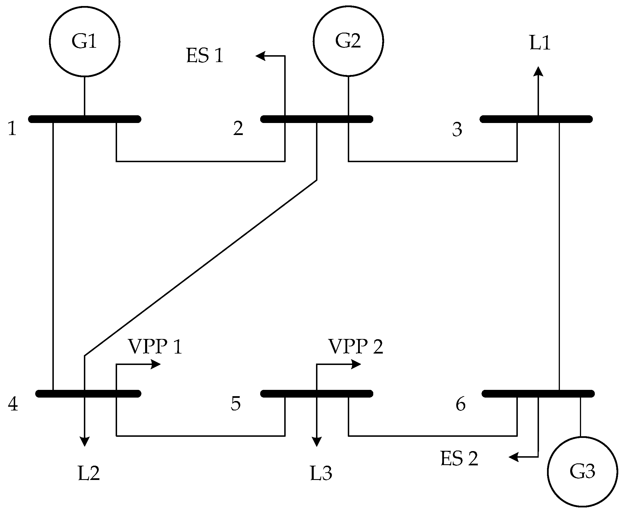
4.1. Six-Bus Test System

The six-bus test system was designed based on the system in [29]. This system has three conventional nonstrategic generators, seven transmission lines, two grid-level ESs, and two IBDR-VPPs. The locations of these components can be found in Figure 2. The LSE owns all the grid-level ESs and IBDR-VPPs in this system. Also, the total power load is assigned to buses 3, 4, and 5 based on the distribution factors (0.5, 0.3, and 0.2, respectively).

To demonstrate the impact of different scenarios on the daily profit of LSE, we designed three cases, where each case consists of several subcases:

• LSE’s basic strategic scheduling with ES and IBDR-VPP in the DA market;
• Impact of ES/ IBDR-VPP outage on LSE’s strategic scheduling without contingency anticipation time (CAT) in the ID market;
• LSE’s remedial strategic scheduling with CAT under the impact of ES/ IBDR-VPP outage.

Case 1:

In this case, the daily profit of the LSE is optimized based on the day-ahead strategic scheduling model established in Section 2.3.1. Since the impact of ES/IBDR-VPP outage is not taken account into this case, the whole system can be seen in normal operating status during the period in question. With a charging price that is obviously lower than the other conventional generator unit marginal costs, ES owners are stimulated to participate in electricity market activities. Thus, we assume that the contract price for ES charging is $25/MW within the first 12 h and $40/MW within the last 12 h. Similarly, the contract price for IBDR-VPP compensation is set at $20/MW within the first 12 h and $35/MW within the last 12 h. Also, $T_{down}^{\min }$ and $T_{up}^{\max }$ are set to 6 h and 4 h, respectively. The LSE’s daily profit is $32,816 in the simulation process. The scheduling of the two VPPs can be seen in

Table 1. Hourly optimal scheduling of VPPs in the modified six-bus test system.

Time	1	2	3	4	5	6	7	8	9	10	11	12
VPP 1	40	0	0	0	0	0	0	26.62	34.48	40	0	0
VPP 2	40	40	38.51	32.57	0	0	0	0	0	0	40	40
Time	13	14	15	16	17	18	19	20	21	22	23	24
VPP 1	0	0	0	0	40	40	40	40	0	0	0	0
VPP 2	40	40	0	0	0	0	0	0	40	40	40	35.06

.

VPP 1 starts at time 8, then stays online for the next three hours which is shorter than $T_{up}^{\max }$. Thus, the VPP does not always stay online until the maximum online hours run out to gain more profit. In contrast, the scheduling of VPPs is to maximize the LSE’s daily profit along with ES scheduling. Also, a subcase without VPPs is simulated to analyze the impact of VPP integration on ES scheduling. Figure 3 shows the comparison between ES scheduling without VPP and with the two VPPs.

It can be observed that the scheduling of ESs is significantly changed with the integration of VPPs. Note that both ESs are in discharging mode at the peak load hour (time 1) and in charging mode at the valley load hour (time 7), regardless of the integration of VPPs, which is consistent with the ES’s original intention of peak-shaving and valley-filling. Also, with 40 MW·h virtual energy of each VPP’s input, the discharging energy of ES 1 reduces from 35 MW·h to 14.62 MW·h, while that of ES 2 reduces from 35 MW·h to 29.35 MW·h at the peak load hour. Thus, the VPP has a supplemental function of peak-shaving and valley-filling when it cooperates with the ES.

Case 2:

In the previous case, the LSE’s daily profit is maximized in the DA market. However, contingencies in the ID market, such as ES outage and insufficient response of VPP, may have consequences for the optimal process, resulting in fluctuations of both ES and VPP scheduling and diminishing profit. Thus, contingencies should be taken into account, since they are an important factor in LSE’s strategic scheduling.

In this paper, the insufficient response of VPP is considered as a VPP outage to simplify the demand response model. Also, virtual generators, ESs, and conventional generators are assumed to participate in the ID market rescheduling process with the rest of their capacities. Compared with case 1, there is a start time t₀ when the specific contingency occurs. Except for this, other parameters remain unchanged. Four contingencies, ES 1 and 2 outage and VPP 1 and 2 outage, are simulated in the case. Under each contingency, two schemes are adopted to maximize the LSE’s daily profit. In scheme 1, we assume that the status (including charging/discharging status of ESs and on/off status of VPPs) of nonoutage units is fixed after a specific outage occurs. The scheduling values are optimized according to the model established in Section 2.3.2. By contrast, both the status and outputs of the units participate in the optimizing process in scheme 2. The ES 1 and 2 outage and VPP 1 and 2 outage are represented by C1, C2, C3, and C4, respectively. Simulations under C2 and C4 outage are selected to illustrate the differences of ES/VPP scheduling between scheme 1 and scheme 2.

Comparisons of ES stored energy and VPP output under the two contingencies are shown in Figure 4 and Figure 5, respectively. It can be observed that each contingency brings a series of consequences to the scheduling of both ES and VPP. LSE’s daily profit in scheme 2 is higher than the profit in scheme 1, which can be found in

Table 2. Daily profit under different contingencies ($).

Contingency No.	C1	C2	C3	C4
Scheme 1	23,556	23,133	29,447	22,167
Scheme 2	23,556	23,605	29,447	27,282

. In other words, rescheduling both the status and output of ESs and VPPs can help the LSE reduce losses caused by ES or VPP outage.

Case 3:

From the perspective of contingency forecasting, it is very helpful for LSEs to take measures ahead of time, i.e., if a specific contingency has been predicted, then the period before the contingency could be adequately utilized to reduce losses with a new schedule.

The remedial strategic scheduling process for the LSE’s daily profit is simulated based on the contingencies listed in case 2. CAT is considered in this case with the contingency anticipation time t_P set to 6–12 consecutively. Also, scheme 2 is selected to reschedule both ESs and VPPs. The quantitative evaluation for the LSE’s daily loss according to the remedial strategic scheduling is shown in

Table 3. LSE’s daily loss with contingency anticipation time in the modified six-bus test system ($).

CAT	tP = 6	tP = 7	tP = 8	tP = 9	tP = 10	tP = 11	tP = 12
C1	–1027	–1629	–2342	–3816	–5470	–7274	–9257
C2	1664	–361	–1925	–2707	–4146	–6528	–9208
C3	–3123	–3123	–3123	–3123	–3123	–3369	–3369
C4	–5287	–5287	–5287	–5287	–5287	–5531	–5531

. It can be observed that the LSE’s loss will generally be lower with more remedial time under all listed contingencies.

It is interesting that under C2, with six hours of the CAT, the LSE’s daily profit is higher than that under the noncontingency scenario. Note that when there is no contingency, ES 2 is in charging status from time 6 to time 12, which results in negative profit for the LSE during this period. It is reasonable from the perspective of the LSE’s daily profit. To have enough energy to trade in the market, ES 2 should choose to charge when there is a lower purchasing price according to the contract. However, once the ES 2 outage has been predicted, ES 2 can change its charging status and provide stored energy to the market as much as possible.

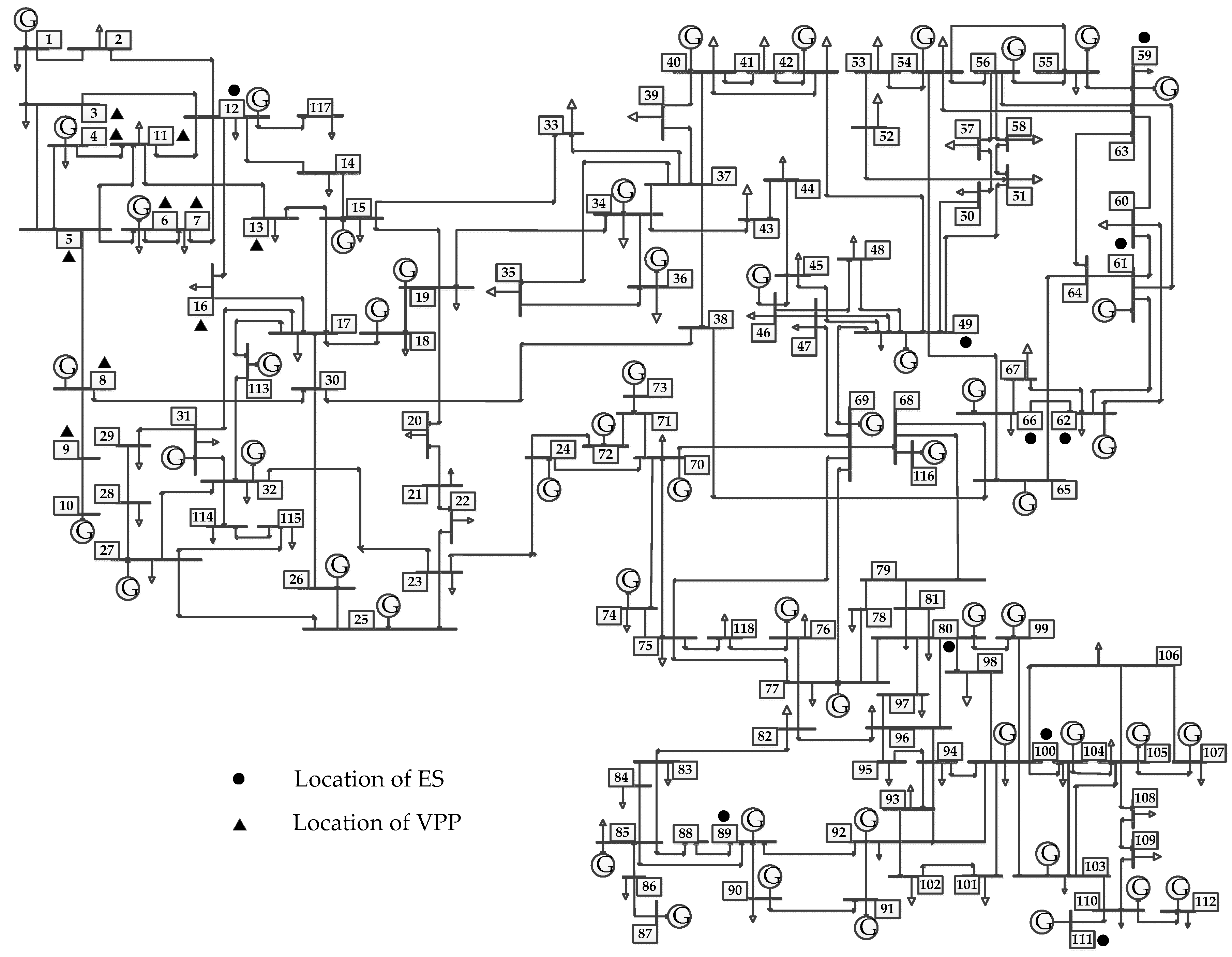
4.2. IEEE 118-Bus Test System

To verify the effectiveness of the proposed model on a large system, a simulation study was also done with a modified IEEE 118-bus system. The system consists of 186 transmission lines and 91 load buses with peak load set to 7 GW. We assume that all IBDR-VPPs and grid-level ESs are owned and dispatched by the LSE; the locations of VPPs and ESs can be seen in Figure 6. The contract price for the ES charging and IBDR-VPP compensation remains the same. $T_{down}^{\min }$ and $T_{up}^{\max }$ are set to 6 h and 4 h, respectively.

The simulation cases include: (1) the LSE’s basic strategic scheduling with ES and IBDR-VPP in the DA market; and (2) the LSE’s remedial strategic scheduling with CAT under the impact of different ES/IBDR-VPP outages.

It can be observed from

Table 4. Hourly optimal scheduling of VPPs in the modified IEEE 118-bus system.

Time	1	2	3	4	5	6	7	8	9	10	11	12
VPP 1	0	0	0	0	0	0	0	0	40	40	40	40
VPP 2	0	0	0	0	0	0	0	40	40	40	40	0
VPP 3	0	0	0	0	0	0	0	0	40	40	40	40
VPP 4	0	0	0	0	0	0	0	0	40	40	40	40
VPP 5	16.8	0	0	0	0	0	0	0	40	40	40	40
VPP 6	40	0	0	0	0	0	0	0	40	40	40	40
VPP 7	0	23.14	0	0	0	0	0	0	40	40	40	40
VPP 8	40	40	0	0	0	0	0	0	40	40	40	40
VPP 9	40	0	0	0	0	0	0	0	40	40	40	40
VPP 10	40	40	0	0	0	0	0	0	40	40	40	40
Time	13	14	15	16	17	18	19	20	21	22	23	24
VPP 1	0	0	0	0	0	0	40	40	40	40	0	0
VPP 2	0	0	0	0	0	0	40	40	40	40	0	0
VPP 3	0	0	0	0	0	0	40	40	40	40	0	0
VPP 4	0	0	0	0	0	0	40	40	40	40	0	0
VPP 5	0	0	0	0	0	0	40	40	40	40	0	0
VPP 6	0	0	0	0	0	0	40	40	40	40	0	0
VPP 7	0	0	0	0	0	0	40	40	40	40	0	0
VPP 8	0	0	0	0	0	0	40	40	40	40	0	0
VPP 9	0	0	0	0	0	0	40	40	40	40	0	0
VPP 10	0	0	0	0	0	0	40	40	40	40	0	0

that the scheduling of VPPs is also reasonable in the IEEE 118-bus test system. Note that VPP 7 starts at time 2 and then shuts down at time 3, which indicates that it stays online for just 1 h (shorter than $T_{up}^{\max }$). Meanwhile, VPP 9 shuts down at time 2 and stays offline for the next 7 h (longer than $T_{down}^{\min }$) until it restarts at time 9. This implies that the VPP does not always stay online within the maximum online hours or restart as soon as the minimum offline hours run out.

The loss-redeeming process utilizing the LSE’s remedial strategic scheduling with CAT is also observed in the IEEE 118-bus test system. VPP and ES outages are represented by C_v,i (i = 1, 2, ··· 10) and C_e,j (j = 1, 2, ···, 12), respectively. To illustrate the effectiveness of the remedial strategic scheduling, typical contingencies are selected, and the corresponding quantitative evaluation for the LSE’s daily loss are listed in

Table 5. LSE’s daily loss with contingency anticipation time in the modified IEEE 118-bus system ($).

CAT	tP = 6	tP = 7	tP = 8	tP = 9	tP = 10	tP = 11	tP = 12
Cv,1	–800	–800	–800	–800	–800	–800	–800
Cv,5	–800	–800	–800	–800	–800	–800	–800
Ce,1	3738	3721	3680	918	918	–2338	–5518
Ce,4	5983	3951	1221	–1103	–1176	–1202	–4357
Ce,9	4616	2058	328	260	–1103	–2921	–2921
Ce,12	4039	1481	1431	1363	–1103	–1825	–5005

.

It can be seen that although daily loss remains the same under the contingencies with VPP outage, it will be significantly reduced with more remedial time under the contingencies with ES outage. Similarly, most ESs in the IEEE 118-bus test system are in charging mode before the contingency happens. Then, because of the LSE’s remedial rescheduling scheme, the operation status of ESs changes, tending to discharge within the CAT. It contributes to the loss redeeming, resulting in extra daily profit for the LSE.

5. Discussion

In this section, the simulation results and working hypotheses are discussed. From the case study above, the following can be observed.

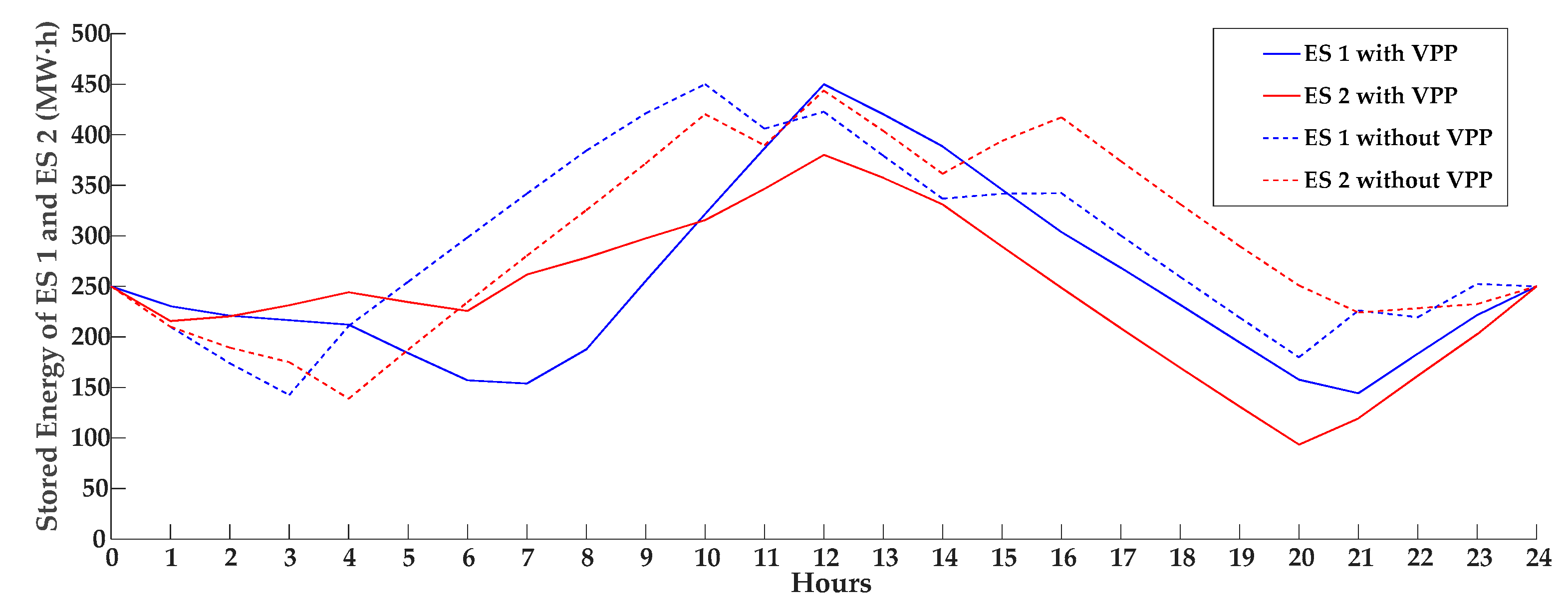
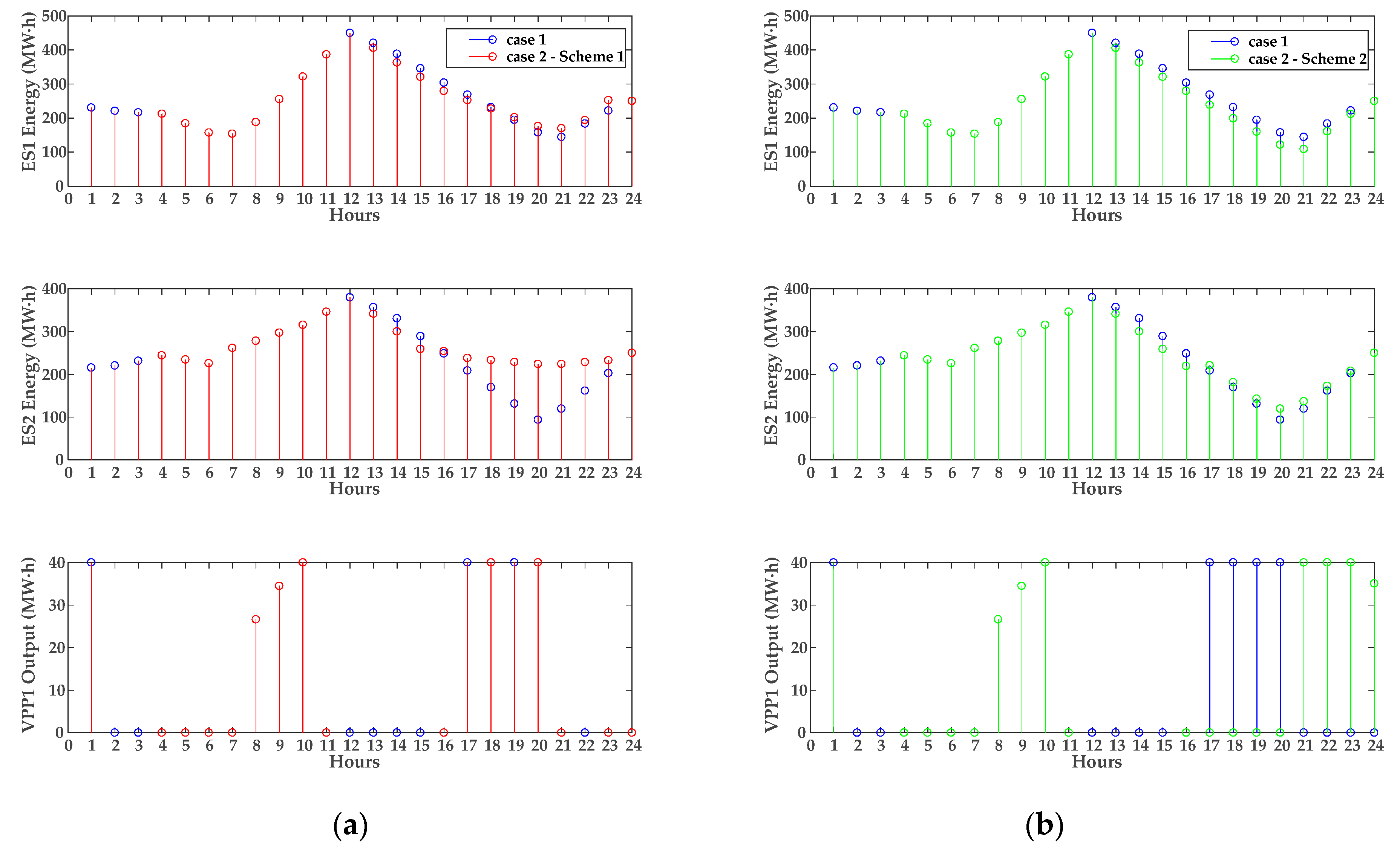
• With the integration of VPPs in the modified six-bus test system, the output of ES 1 reduces from 35 MW·h to 14.62 MW·h (58.22% lower), and the output of ES 2 reduces from 35 MW·h to 29.35 MW·h (16.14% lower) at the peak load hour. The VPPs significantly support the ESs (especially ES 1) on the peak-shaving objective.
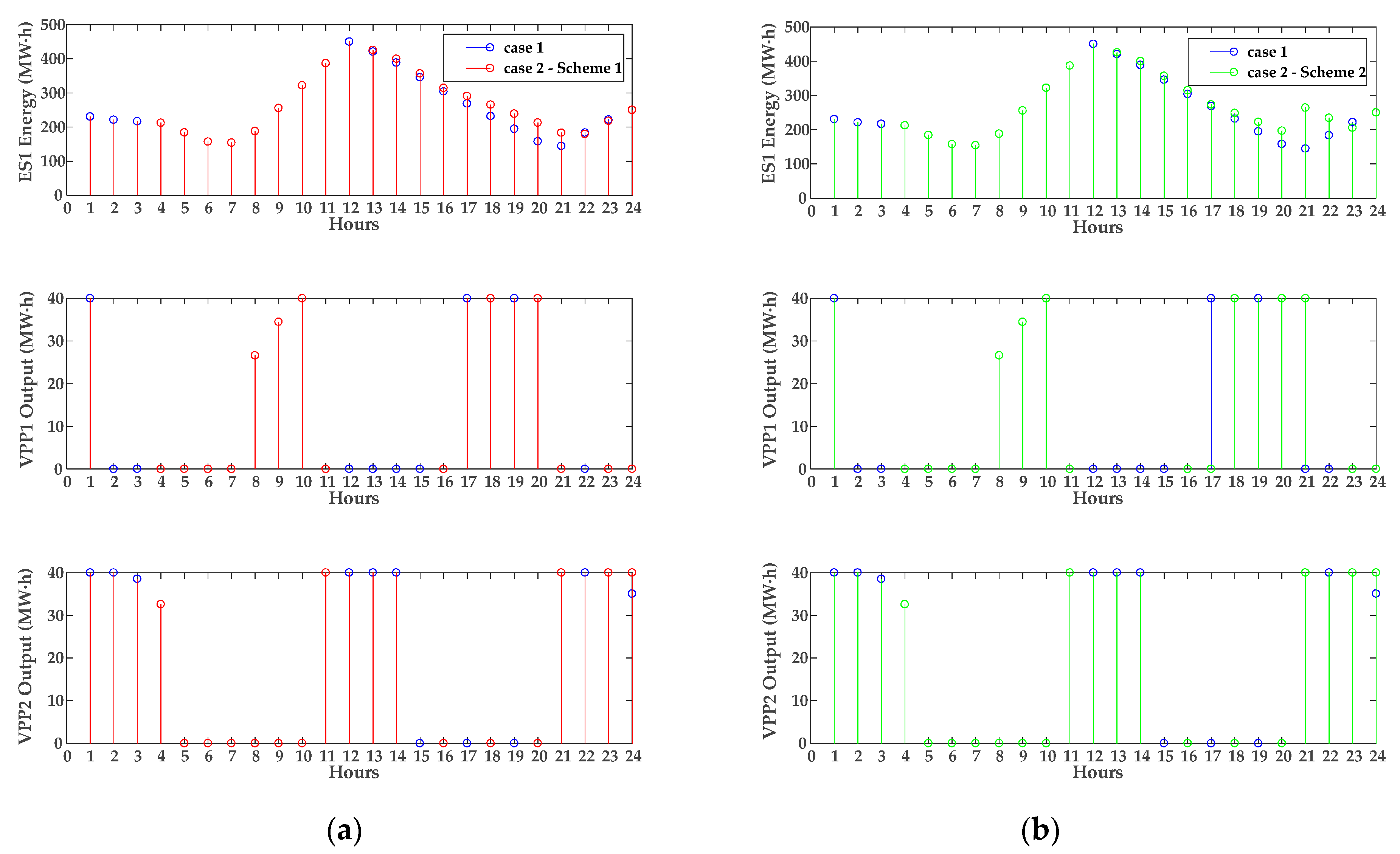
• With the rescheduling process in the ID market, LSEs can reduce more losses using scheme 2 than scheme 1. For instance, under the ES 2 outage and VPP 2 outage in the modified six-bus test system, the LSE’s daily profits after using scheme 1 as the rescheduling strategy are $23,133 and $22,167, respectively. By contrast, the daily profits with scheme 2 are $23,605 ($472 higher) and $27,282 ($5115 higher), respectively.
• With more contingency anticipation hours, the LSE will further reduce the losses based on the proposed remedial strategic scheduling approach. Typical results are selected to illustrate this viewpoint. In the modified six-bus test system, under the ES 1 outage, the daily losses of the LSE with 6 h CAT and 1 h CAT are $1027 and $7274, respectively. In the modified IEEE 118-bus test system, under the ES 4 outage, the daily losses of the LSE with 3 h CAT and 1 h CAT are $1103 and $4357, respectively.

In addition, hypotheses are made regarding the LSE’s remedial strategic scheduling model. In the model, we assume that the contingency anticipation time can be provided by the sensor. It is a reasonable hypothesis due to the advancement of failure detection and communication technology. Meanwhile, we assume that in the simulation process of remedial scheduling, the outage recovery cost, like the ES’s maintenance cost, is not included. It becomes a limitation of the model presented here. It is also another important reason why, under several contingencies of both the modified six-bus test system and IEEE 118-bus test system, the losses are negative after utilizing the remedial strategic scheduling approach, i.e., if the recovery cost were considered and set high enough, the LSE would not gain profit. However, the recovery cost is difficult to judge, since it contains many uncertainties related to the occurrence probability and severity of a specific outage. Also, this paper is focused on a quantitative assessment of the LSE’s loss reduction after using the remedial strategic scheduling approach. Thus, considering model complexity and computation efficiency, we simplify the model of the remedial strategic scheduling. However, it is definitely a significant extension for this work.

In the future, we plan to combine the risk probability with our framework and make the proposed model appropriate for the scenario considering uncertainties.

6. Conclusions

In this paper, a remedial strategic scheduling approach for the daily profit of LSEs is presented based on a bilevel optimization model. First, a day-ahead strategic scheduling model with the interaction of grid-level ESs and IBDR-VPPs is established. Second, the intraday rescheduling model considering ESs and VPPs is integrated into the LSE’s daily profit model. Finally, the remedial strategic scheduling approach considering contingency anticipation time is modeled, and case studies demonstrate the quantitative loss assessment.

From work presented in this paper, general conclusions are made as follows:

• VPP integration has a notable impact on ES scheduling. Meanwhile, when coordinated with ES, VPP has a supplemental function of peak-shaving and valley-filling.
• The rescheduling process in the ID market is capable of reducing the LSE’s loss caused by contingencies. Also, the LSE will further reduce the loss with more contingency anticipation time based on the remedial strategic scheduling approach.
• The remedial approach provides a quantitative assessment of the LSE’s loss redeeming, which can be applied in the power system dispatching to help the LSE deal with contingencies.

References

1. Karim, M.E.; Munir, A.; Karim, M.A.; Muhammad-Sukki, F.; Abu-Bakar, S.; Sellami, N.; Bani, N.; Hassan, M. Energy Revolution for Our Common Future: An evaluation of the emerging international renewable energy law. Energies 2018, 11, 1769. [Google Scholar] [CrossRef]
2. Baharvandi, A.; Aghaei, J.; Niknam, T.; Shafie-Khah, M.; Godina, R.; Catalao, J. Bundled generation and transmission planning under demand and wind generation uncertainty based on a combination of robust and stochastic optimization. IEEE Trans. Sustain. Energy 2018, 9, 1477–1486. [Google Scholar] [CrossRef]
3. Acuna, L.; Padilla, R.; Mercado, A. Measuring reliability of hybrid photovoltaic-wind energy systems: A new indicator. Renew. Energy 2017, 106, 68–77. [Google Scholar] [CrossRef]
4. Mazzeo, D.; Oliveti, G.; Baglivo, C.; Congedo, P. Energy reliability-constrained method for the multi-objective optimization of a photovoltaic-wind hybrid system with battery storage. Energy 2018, 156, 688–708. [Google Scholar] [CrossRef]
5. Mohamad, F.; Teh, J. Impacts of energy storage system on power system reliability: A systematic review. Energies 2018, 11, 1749. [Google Scholar] [CrossRef]
6. Hatwig, K.; Kockar, I. Impact of strategic behavior and ownership of energy storage on provision of flexibility. IEEE Trans. Sustain. Energy 2016, 7, 744–754. [Google Scholar] [CrossRef]
7. Pieroni, T.; Dotta, D. Identification of the most effective point of connection for battery energy systems focusing on power system frequency response improvement. Energies 2018, 11, 763. [Google Scholar] [CrossRef]
8. Rodrigues, E.; Godina, R.; Catalao, J. Modelling electrochemical energy storage devices in insular power network applications supported on real data. Appl. Energ. 2017, 188, 315–329. [Google Scholar] [CrossRef]
9. Hidalgo-Leon, R.; Siguenza, D.; Sanchez, C.; Leon, J.; Jacome-Ruiz, P.; Wu, J.; Ortiz, D. A survey of battery energy storage system (BESS), application and environmental impacts in power systems. In Proceedings of the IEEE Second Ecuador Technical Chapters Meeting (ETCM), Salinas, Ecuador, 16–20 October 2017. [Google Scholar]
10. Farhadi, M.; Mohammed, O. Energy storage systems for high power applications. In Proceedings of the Industry Applications Society Annual Meeting, Addison, TX, USA, 18–22 October 2015. [Google Scholar]
11. Rahmann, C.; Mac-Clure, B.; Vittal, V.; Valencia, F. Break-even points of battery energy storage systems for peak shaving applications. Energies 2017, 10, 833. [Google Scholar] [CrossRef]
12. Krishnamurthy, D.; Uckun, C.; Zhou, Z.; Thimmapuram, P.; Botterud, A. Energy storage arbitrage under day-ahead and real-time price uncertainty. IEEE Trans. Power Syst. 2018, 33, 84–93. [Google Scholar] [CrossRef]
13. Cui, H.; Li, F.; Fang, X.; Chen, H.; Wang, H. Bilevel arbitrage potential evaluation for grid-scale energy storage considering wind power and LMP smoothing effect. IEEE Trans. Sustain. Energy 2018, 9, 707–718. [Google Scholar] [CrossRef]
14. Khani, H.; Mohannad, R.; Zadeh, D. Real-time optimal dispatch and economic viability of cryogenic energy storage exploiting arbitrage opportunities in an electricity market. IEEE Trans. Smart Grid 2015, 6, 391–401. [Google Scholar] [CrossRef]
15. Luburic, Z.; Pandzic, H.; Plavsic, T. Assessment of energy storage operation in vertically integrated utility and electricity market. Energies 2017, 10, 683. [Google Scholar] [CrossRef]
16. Zhang, G.; Jiang, C.; Wang, X.; Li, B.; Zhu, H. Bidding strategy analysis of virtual power plant considering demand response and uncertainty of renewable energy. IET Gener. Transm. Distrib. 2017, 11, 3268–3277. [Google Scholar] [CrossRef]
17. Shi, Q.; Cui, H.; Li, F.; Liu, Y.; Ju, W.; Sun, Y. A hybrid dynamic demand control strategy for power system frequency regulation. CSEE J. Power Energy Syst. 2017, 3, 176–185. [Google Scholar] [CrossRef]
18. Wei, C.; Xu, J.; Liao, S.; Sun, Y.; Jiang, Y.; Ke, D.; Zhang, Z.; Wang, J. A bi-level scheduling model for virtual power plants with aggregated thermostatically controlled loads and renewable energy. Appl. Energy 2018, 224, 659–670. [Google Scholar] [CrossRef]
19. Abbasi, E. Coordinated primary control reserve by flexible demand and wind power through ancillary service-centered virtual power plant. Int. Trans. Electr. Energy 2017, 27, 1–18. [Google Scholar] [CrossRef]
20. Garcia-Gonzalez, J.; De La Muela, R.; Santos, L.; Gonzalez, A. Stochastic joint optimization of wind generation and pumped-storage units in an electricity market. IEEE Trans. Power Syst. 2008, 23, 460–468. [Google Scholar] [CrossRef]
21. Akhavan-Hejazi, H.; Mohsenian-Rad, H. Optimal operation of independent storage systems in energy and reserve markets with high wind penetration. IEEE Trans. Smart Grid 2014, 5, 1088–1097. [Google Scholar] [CrossRef]
22. Mnatsakanyan, A.; Kennedy, S. A novel demand response model with an application for a virtual power plant. IEEE Trans. Smart Grid 2015, 6, 230–237. [Google Scholar] [CrossRef]
23. Al-Awami, A.; Amleh, N.; Muqbel, A. Optimal demand response bidding and pricing mechanism with fuzzy optimization: application for a virtual power plant. IEEE Trans. Ind. Appl. 2017, 53, 5051–5061. [Google Scholar] [CrossRef]
24. Wang, Y.; Ai, X.; Tan, Z.; Yan, L.; Liu, S. Interactive dispatch modes and bidding strategy of multiple virtual power plants based on demand response and game theory. IEEE Trans. Smart Grid 2016, 7, 510–519. [Google Scholar] [CrossRef]
25. Ott, A. Experience with PJM market operation, system design, implementation. IEEE Trans. Power Syst. 2003, 18, 528–534. [Google Scholar] [CrossRef]
26. Analui, B.; Scaglione, A. A dynamic multistage stochastic unit commitment formulation for intraday markets. IEEE Trans. Power Syst. 2018, 33, 3653–3663. [Google Scholar] [CrossRef]
27. Weber, C. Adequate intraday market design to enable the integration of wind energy into the European power systems. Energy Policy 2010, 38, 3155–3163. [Google Scholar] [CrossRef]
28. Soysal, E.; Olsen, O.; Skytte, K.; Sekamane, J. Intraday market asymmetries—A Nordic example. In Proceedings of the 2017 14th International Conference on the European Energy Market (EEM), Dresden, Germany, 6–9 June 2017. [Google Scholar]
29. Cui, H.; Li, F.; Hu, Q.; Bai, L.; Fang, X. Day-ahead coordinated operation of utility-scale electricity and natural gas networks considering demand response based virtual power plants. Appl. Energy 2016, 176, 183–195. [Google Scholar] [CrossRef] [Green Version]
Figure 1. Overview of the remedial strategic scheduling model. ES, energy storage; IBDR-VPP, interruptible load-based demand response virtual power plant; LSE, load serving entity.
Energies 11 02420 g001
Figure 2. Topology of the modified six-bus test system.
Energies 11 02420 g002
Figure 3. Stored energy of ESs with/without VPP integration.
Energies 11 02420 g003
Figure 4. Comparisons of ES 1 stored energy, VPP 1 output, and VPP 2 output under C2. (a) ES 1 stored energy, VPP 1 output, and VPP 2 output in case 1 and case 2 (with scheme 1); (b) ES 1 stored energy, VPP 1 output, and VPP 2 output in case 1 and case 2 (with scheme 2).
Energies 11 02420 g004
Figure 5. Comparisons of ES 1 stored energy, ES 2 stored energy, and VPP 1 output under C4. (a) ES 1 stored energy, ES 2 stored energy, and VPP 1 output in case 1 and case 2 (with scheme 1); (b) ES 1 stored energy, ES 2 stored energy, and VPP 1 output in case 1 and case 2 (with scheme 2).
Energies 11 02420 g005
Figure 6. Topology of the modified IEEE 118-bus test system.
Energies 11 02420 g006