Article

Heat Transfer Behaviors in Horizontal Wells Considering the Effects of Drill Pipe Rotation, and Hydraulic and Mechanical Frictions during Drilling Procedures

1
State Key Laboratory of Geomechanics and Geotechnical Engineering, Institute of Rock and Soil Mechanics, Chinese Academy of Science, Wuhan 430071, Hubei, China
2
University of Chinese Academy of Sciences, Beijing 100049, China
3
State Key Laboratory of Oil and Gas Reservoir Geology and Exploitation, Southwest Petroleum University, Chengdu 610500, Sichuan, China
4
PetroChina Co. Ltd., Chuandong Drilling Company, Chongqing 401147, China
5
CNOOC Ltd., Zhanjiang Branch, Zhanjiang 524057, Guangdong, China
*
Authors to whom correspondence should be addressed.
Energies 2018, 11(9), 2414; https://doi.org/10.3390/en11092414
Submission received: 30 August 2018 / Revised: 7 September 2018 / Accepted: 10 September 2018 / Published: 12 September 2018

Abstract

:
Horizontal wells are increasingly being utilized in the exploration and development of oil and gas resources. However, the high temperature that occurs during drilling processes leads to a number of problems, such as the deterioration of drilling fluid properties and borehole instability. Therefore, the insight into heat transfer behaviors in horizontal wells is certainly advantageous. This study presents an integrated numerical model for predicting the temperature distribution during horizontal wells drilling considering the effects of drill pipe rotations, and hydraulic (i.e., circulating pressure losses) and mechanical frictions. A full implicit finite difference method was applied to solve this model. The results revealed that the mechanical frictions affect more on wellbore temperature variation than the effects of heat transfer intensification and circulating pressure losses; Moreover, the drilling fluid temperature was found higher than the stratum temperature at horizontal section, the temperature difference at the bottom hole reached up to 16 °C if pressure drops, heat transfer strengthened by rotations and mechanical frictions were all taken into account. This research could be utilized as a theoretical reference for predicting temperature distributions and estimating risks in horizontal wells drilling.

1. Introduction

The circulating temperature in the wellbore during the drilling procedure is a matter worth examining. The circulating temperature inevitably affects the properties of operating fluids during the drilling of oil–gas wells, and temperature fluctuations in the wellbore and formations expose the surrounding rocks to the risk of collapse. Moreover, temperature impacts the creep rates of soft rock interlayers, such as salt, gypsum, and mudstone. In addition, the corrosion of downhole tools and expansion of gas flowing with the drilling fluid are known to be related to the temperature profile. All these aspects mentioned above significantly affect well safety during drilling.
It is generally difficult to predict the downhole temperature profile during the drilling procedure because of the complex and volatile drilling conditions. In previous decades, several studies were conducted on wellbore temperature. Edwardson [1] presented a method to approximately predict wellbore and formation temperature. Ramey et al. [2] introduced a time function, f(t), and total heat transfer coefficient, and computed the circulating temperature considering fluid injection. Their study laid the foundation for further research on wellbore temperature. Holmes and Swift [3], and Arnold [4] deduced an analytical model for estimating wellbore temperature under a steady state. Hasan and Kabir [5], inspired by the law of pore pressure diffusion in formations, categorized the thermal conduction in formations as radial, one-dimensional, and steady-state heat transfers, and used the inversion of the Laplace transformation to understand the temperature distribution in rocks around wellbores. Furthermore, they modified the time function f(t), which was subsequently widely applied [6,7]. Based on the studies of Ramey [2], and Holmes and Swift [3], Kabir and Hasan [7] established a temperature model for reverse circulation. Aniket et al. [8], and Kumar and Samuel [9] focused on extended-reach drilling and casing while drilling, respectively. Moreover, they introduced an analytical model, including a friction heat source between the drill pipe and wellbore wall, into the model of Kabir and Hasan. The study of Livescu and Wang [10] provided an insight on the wellbore temperature during coiled tubing drilling. The aforementioned investigations were mainly conducted on the basis of analytical methods. With the development of computational technology, further numerical methods were introduced to calculate the wellbore temperature during the drilling procedure. Raymond [11] derived energy equations for the fluid in the drill pipe and annulus, as well as in surrounding rocks by utilizing the finite element method to obtain the numerical solution of the temperature profile under steady and pseudo-steady states. Latterly, Keller [12] provided detailed discrete forms of energy equations, taking into consideration integral wellbore geometric structures, including cement sheaths and casing pipes. Marshall and Bentsen [13] applied a different formula to determine the effects of circulating pressure losses on temperature in the drill pipe, annulus, and drill bit. The study assumed turbulent flow in the drill pipe and laminar flow in the annulus. The drilling fluid was treated as a power-law fluid. Recent research continued to focus on temperature distribution during well drilling. Song and Guan [14] proposed a temperature–pressure coupling model for aerated underbalanced drilling in deep water. Yang [15] probed the wellbore-stratum temperature, which encountered the loss of drilling fluid. In addition to the finite element method mentioned above, other solving algorithms were still applied, such as the finite volume method [16,17], artificial neural network [18], and semi-analytical method [19].
For the temperature profiles of horizontal wells, Siu and Li [20], Yoshioka and Zhu [21,22], and Muradov and Davies [23] examined the temperature distribution of horizontal segments when fluids flowed into or from formations. For the drilling procedure, Trichel and Fabian [24] investigated high-temperature horizontal wells and discussed energy loss during drilling. A field engineering software was used to calculate torque, drag force, and hydraulic friction. However, certain equations and properties of the drilling fluid were not clear. Nguyen and Miska [25], who made derivations based on the investigation conducted by Kabir and Hasan on the temperature of a vertical well and considered the mechanical friction between drill pipes and wellbore wall, employed an analytical model to predict the circulating temperature of horizontal wells, but ignored the effect of hydraulic friction. The work completed by Li and Liu [17] on the temperature of horizontal wells included information on the heat source of viscous dissipation, which was similar to the hydraulic friction in drilling fluids and other mechanical frictions. Nevertheless, the study would have been more comprehensive if the effect of the key parameter, Nu, was considered. Therefore, for horizontal wells it is advantageous to delve into the integrated impact of all heat sources induced by wellbore geometry and drilling fluid circulation.
In this study, a comprehensive numerical model intended for estimating wellbore and formation temperature distribution during horizontal well drilling was established according to the law of conservation of energy, and a five-point finite difference scheme was employed in the solution process. The drilling fluid was treated as a non-Newtonian yield-power-law fluid, which accorded with the behavior of drilling fluid used at the site. Moreover, the effects of drill pipe eccentricity and drill pipe rotation on the heat transfer procedure in horizontal wells were taken into account. Accordingly, not only were conventional operational parameters related to wellbore temperature, for instance, circulating time, displacement, and geothermal gradient, considered, but also other factors that influenced mechanical and hydraulic frictions, such as heat transfer efficiency, drill pipe eccentricity and rotation. This study was aimed at providing an accurate prediction of temperature distributions in wellbores and formations during horizontal well drilling.

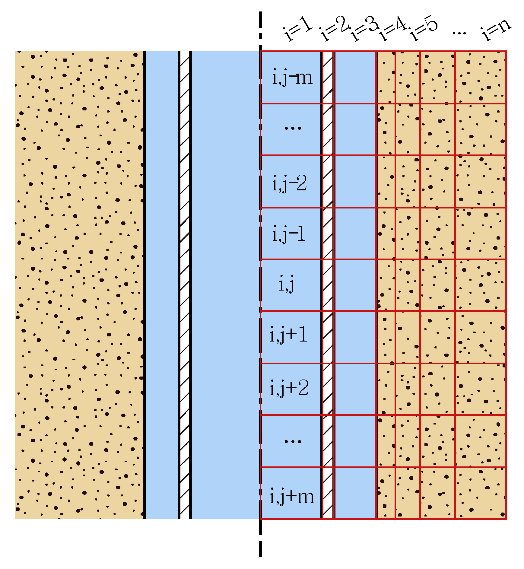
2. Wellbore Geometry and Heat Transfer Mathematical Model

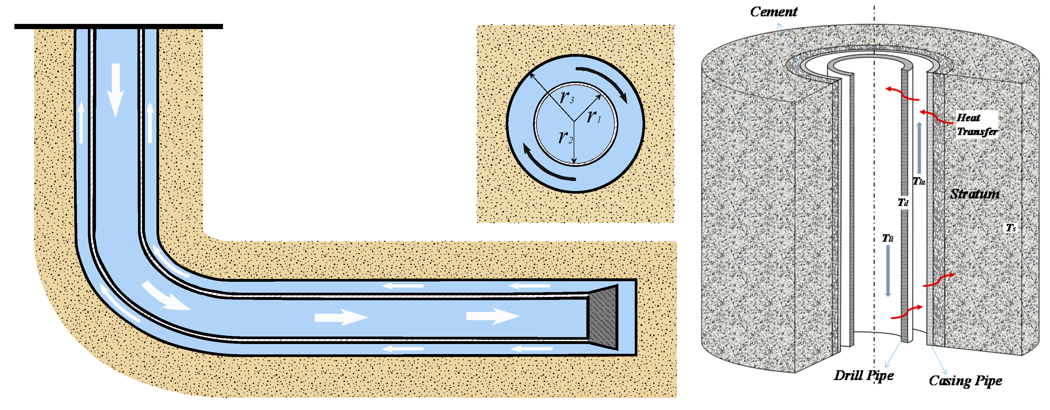
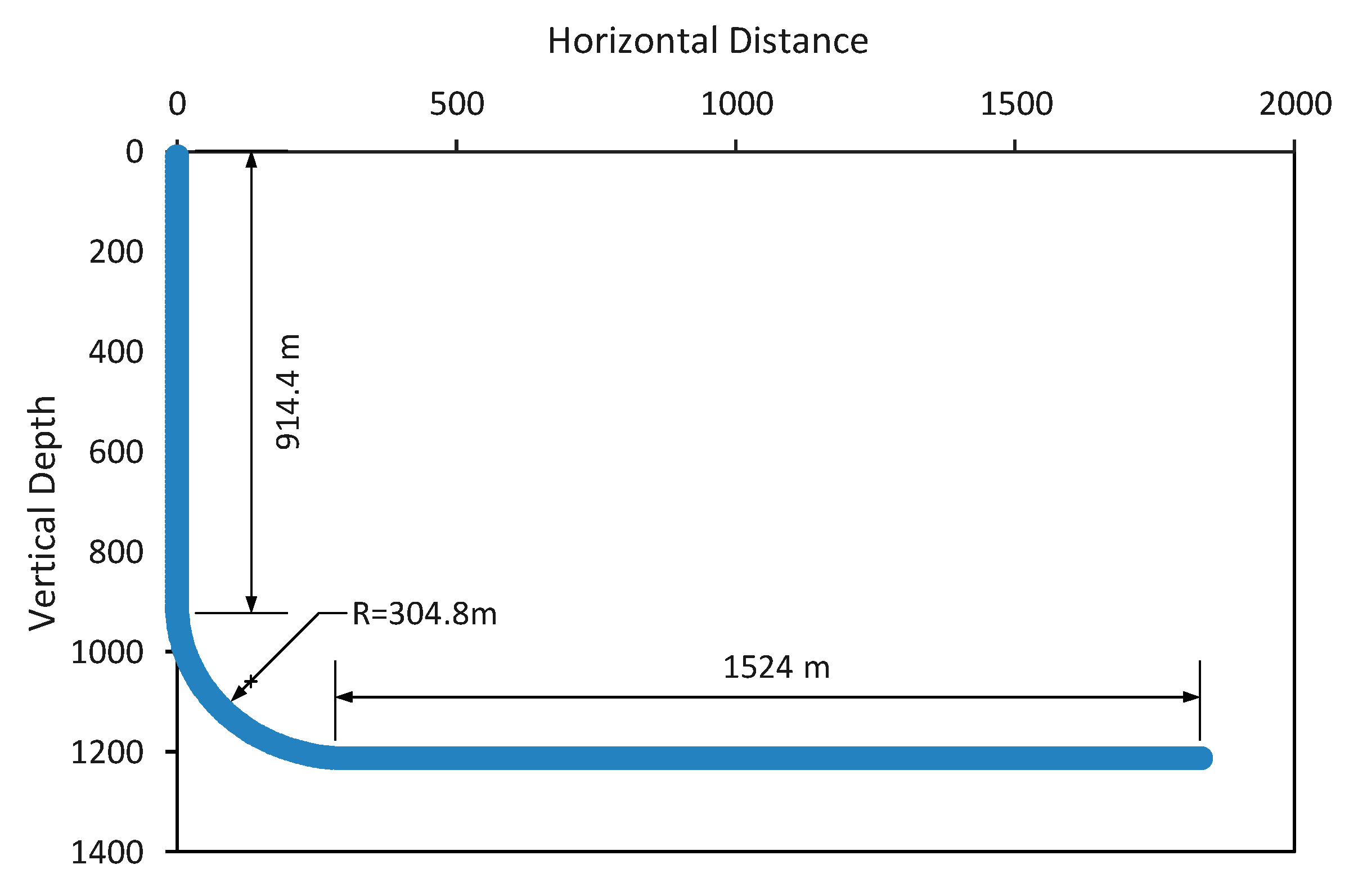
2.1. Description of Wellbore Geometry

Figure 1 shows the wellbore geometry of a horizontal well, mainly including the drill pipe, column space in the drill pipe, annulus space between the outer drill pipe wall and wellbore wall, drill bit, and surrounding rock. The drilling fluid flowed down from ground surface within the drill pipe and through the drill bit, and thereafter flowed up along the annulus space, and eventually, was back to the ground surface. The heat transfer, in the form of conduction within solid parts and convection within fluid zones, the same as that between fluids and solids, always occurred during the whole process of circulating and drilling. The practical wellbore geometry was very complex, and the size and shape of the wellbore and annulus were affected by the motion, deformation and rotation of drill pipes. Moreover, other factors, such as lithological characters, drilling rate, and weight on the bit also made differences. Therefore, the trajectory and shape of the annulus were not as regular as those shown in Figure 1.
Some assumptions for our model require introduction, as follows:
(1)
For horizontal wells, the drill pipes in vertical segments were either concentric or eccentric at a constant eccentricity. Built-up segments were linearly and increasingly eccentric along the wellbore axis, with the eccentricity increasing from e = 0, at the kick-off point, to e = 1, at the heel of the horizontal segment; the mean eccentricity was e = 0.62. The horizontal segments were totally eccentric (e = 1).
(2)
No buckling segments existed along the entire well, and the shapes of drill pipes and annuli were regular.
(3)
The effect of casing pipes was not considered as its high heat conductivity. Moreover, the effects of heat radiation and conduction in the drilling fluid along the depth direction were neglected, merely considering the main forms of heat transfer conduction in solid parts and convection in fluid zones.
(4)
The initial geothermal temperature in the formation along the depth linearly increased. Based on the above assumptions, the heat transfer model was established according to the law of thermodynamic energy conservation. Accordingly, they were used to estimate the temperature variation during the drilling procedure.

2.2. Mathematical Model of Heat Transfer

According to works [13,15,17], the first three assumptions enumerated above primarily pertained to the temperature of vertical wells. Although Li [17] analyzed the temperature of horizontal wells, the investigation did not include the effect of hydraulic friction, which was different from what we conducted in this study. As described in Section 2.1, heat transfer not only occurred within solid parts and fluid zones, but also transpired at interfaces between solids and fluids. In this section, the segregation of a small segment, dz, along the depth direction in order to derive the mathematical heat transfer model for each part is discussed.

2.2.1. Thermal Equilibrium Equations

(1) Drilling Fluid in drill pipes:
c l ρ l q T l i z + α d i 2 π r 1 ( T d T l i ) + Q i = c l ρ l π r 1 2 T l i t  
In the above, cl is the specific heat of the drilling fluid; ρl is the drilling fluid density; q is the circulating volume flow rate; r1 is the inner radius of the drill pipe; Tli and Td are the temperature of the drilling fluid in the drill pipe and annulus, respectively; αdi is the convective heat-transfer coefficient at the inner face of the drill pipe; Qi is the heat source from the drill pipe; z is the well depth; t is the circulating time.
(2) Drill pipe:
λ d 2 T d z 2 + 2 r 1 α d i r 2 2 r 1 2 ( T l i T d ) 2 r 2 α d o r 2 2 r 1 2 ( T d T l a ) = c d ρ d T d t  
Here, λd and cd are the heat conductivity coefficient and specific heat of the drill pipe wall, respectively; ρd is the drill pipe density; Td is the temperature of the drill pipe, and Tla is the drilling fluid temperature in the annulus; αdi and αdo are the convective heat-transfer coefficients at the inner and outer faces, respectively.
(3) Drilling Fluid in annular sections:
c l ρ l q T l a z + α d o 2 π r 3 ( T b T l a ) α b 2 π r 2 ( T l a T d ) + Q o = c l ρ l ( r 3 2 r 2 2 ) T l a t  
In this equation, Tb is the temperature at the wellbore wall; αb is the convective heat-transfer coefficient at the wellbore wall; Qo is the heat source in the annulus; r3 is the outer radius of the annulus.
(4) Formation:
T r t = α ( 2 T r r 2 + 1 r T r r + 2 T r z 2 )  
In the above expression, α = λr/(Crρr); Tr is the stratum temperature; r is the radius from the wellbore axis to a certain point in the stratum; λr is the heat conductivity coefficient of the rock; Cr is the specific heat of the rock; ρr is the rock density.

2.2.2. Boundary and Initial Conditions

Boundary and initial conditions were required for solving the heat transfer model. Because the ground surface temperature was not difficult to determine, the initial temperature in the formation, which increased linearly, was determined as well. The inlet temperature of the drilling fluid at the well head was similarly detectable. The temperature at a certain distance from the wellbore axis was always undisturbed and retained the initial state. The temperature at the borehole bottom was equal to that in the drilling fluid in the drill pipe and annulus, and drill pipe wall. In addition, an important coupled boundary, which was the quantity of heat that went through the formation into the borehole by heat conduction, was equal to that of the drilling fluid in the annulus, absorbed from the wellbore wall by heat convection.
(1)
Boundary conditions:
  • Inlet condition: T l i | z = 0 , t = t = T i n ;
  • Temperatures at the wellbore bottom: T l i | z = H , t = t = T d | z = H , t = t = T l a | z = H , t = t ;
  • Coupled conditions at the wellbore wall: α b ( T r T l a ) | r = r b = λ r ( T r r ) | r = r b ;
  • Far field boundary: T r = T s u r f + G T H ( r );
(2)
Initial conditions:
  • Stratum retaining the original temperature: T r = T s u r f + G T H ;
  • Drilling fluid in the drill pipe: T l i = T i n + G f H ;
  • Drilling fluid in the annulus: T l a = T o u t + G f H ;
The heat exchange model mentioned above was solved by the finite difference method, and the wellbore-stratum temperature field was determined after iteration. It was worth noting that the heat sources, i.e., the heat generated by the circulating pressure drop and mechanical friction between the drill pipe and wellbore wall, were considered in this model. However, before the model was solved, it was discretized. Details are provided in Appendix A1.

2.3. Calculation of Heat Transfer Coefficients

2.3.1. Methods of Determining Heat Transfer Coefficients in Previous Studies

The convective heat transfer coefficient was generally determined by a dimensionless number, the Nusselt number, Nu. For the heat transfer in the drill pipe, Nu, differed from that in the annulus. Different types of experimental methods were designed to determine Nu, whose value varied under different experiments. As for forced convective heat transfer, Nu was related to two other dimensionless numbers—Reynolds number, Re, and Prandtl number, Pr, and can be expressed as Nu = f(Re,Pr). These numbers can be computed using the following equations: Nu = αDH, Re = ρvDH, Pr = μCp. In this paper, the methods for determining Nu were reviewed.
(1) Determination of Nu in the drill pipe
● Laminar Regime:
N u = 4.36   o r   4.364 f o r q s = c o n s t a n t N u = 3.66 f o r T s = c o n s t a n t
Some scholars [26,27,28,29,30,31] utilized the first unchanged Nu (Nu = 4.364) when they investigated the laminar flow in drill pipes with a constant qs (i.e., qs = constant), as shown in Equation (5). Keller [12], and Mashall and Bentsen [13] selected a smaller value, i.e., Nu = 4.12. Moreover, Petersen [32] and Li [17] used a coefficient that was dependent on the flow pattern index of the drilling fluid. Specifically,
N u = 4.364 ( ( 3 n + 1 ) / 4 n ) 0.323  
● Turbulent Regime:
Dittus and Boelter [33] introduced Equation (7) as a simplified model for calculating Nu in turbulent pipe flow:
N u =   0 . 023   R e 4 / 5 P r n ( n = 0.4   f o r   h e a t i n g ,   0.3 f o r   c o o l i n g )
Equation (7) is applicable when Re > 104, 0.7 ≤ Pr ≤ 160, and L/D ≥ 10. Moreover, if Re was computed using DH, then this would be the same as the formula utilized by Santoyo-Gutierrez [26] to estimate Nu in the annulus flow under the turbulent regime. This expression had been widely used because of its brevity.
Based on the expression of Dittus and Boelter, Seider and Tate [34] took into consideration the variation in fluid properties. Thus, the term (μ/μs)0.14 to correlate the expression of Dittus and Boelter was introduced:
N u = 0.027 R e 4 / 5 P r 1 / 3 ( μ / μ s ) 0.14 ( R e > 10 4 ; 0.7 P r 16700 ; L / D 10 )
The above formula is simple but not more precise than that what Petukhov [35] proposed, which is Equation (9) below:
N u = ( f / 8 ) R e P r 1.07 + 12.7 ( f / 8 ) 1 / 2 ( P r 2 / 3 1 ) 10 4 < R e < 5 × 10 6 ; 0.5 < P r < 200
where f is the friction coefficient, which can refer to that of the Moody plate. For a smooth tube, f = [1.82log(Re) − 1.64]−2. The equation provided by Petukhov was appropriate only when the flow was fully turbulent, i.e., when Re > 104. Subsequently, Gnielinski [36] applied it to the transitional flow regime (2300 < Re < 104):
N u = ( f / 8 ) ( R e 1000 ) P r 1 + 12.7 ( f / 8 ) 1 / 2 ( P r 2 / 3 1 ) 2300 < R e < 5 × 10 6 ; 0.5 < P r < 200 S m o o t h P i p e : f = ( 0.79 l n R e 1.64 ) 2
Gnielinski [36,37] also introduced the entrance correction factor, 1 + (D/L)2/3, to correlate the effect of the entrance side, as well as another factor, (Pr/Prw)0.11, to correlate with the variation in fluid property. The factor f obtained by various studies differed, such as f = [1.8log(Re) − 1.5]−2 [29,37]. Yang [31], used the formula of Gnielinski with another expression of factor f, and obtained the expression below:
f = a / R e b ( a = ( l o g ( n ) + 3.93 ) / 50 ; b = ( 1.75 l o g ( n ) ) / 7 )
● Transitional Regime
As for Nu under the transitional regime, the same formula for turbulent flow was used by some to determine number. However, the most popular expression was the correlated equation recommended by Gnielinski [26,27,30,31], although there were others who employed linear interpolation to calculate Nu [29,38]:
N u = ( 1 γ ) N u c r i t , l a m + γ N u c r i t , t u r b γ = R e R e c r i t , L a m R e c r i t , T u r b R e c r i t , L a m ( 1 γ 1 )
where Nucrit,Lam and Recrit,Lam are the critical Nusselt and Reynolds numbers from the laminar regime to transitional regime, respectively. Similarly, Recrit,Turb and Nucrit,Turb are the critical Nusselt and critical Reynolds numbers from the transitional regime to turbulent regime.
(2) Determination of Nu in the Annulus
● Laminar Regime
In drill engineering, two methods were used to determine Nu in the annulus. The first was the same as the laminar flow drill pipe Nu, which was equal to 4.364 [30] or 4.12 [12,13]; the second was the widely used expression formulated by Seder and Tate [17,26,31,39], with the factor μ/μw set to 1 when the change in fluid property was not considered:
N u = 1.86 ( R e P r ) 1 3 ( D H L ) 1 3 ( μ μ w ) 0.14 R e < 2300 ; 0.48 < P r < 16700 ; R e P r ( D H / L ) > 10
● Turbulent Regime
In early research, Nu for turbulent flow in the annulus was generally calculated by means of the formula of Dittus and Boelter [33] or that of Seider and Tate [34] with the factor (μ/μs)0.14. In later studies, the expression deduced by Gnielinski or some other derivative equations were applied. Gnielinski [37] presented another expression to consider the effects of the inlet side, variation in the fluid property, and boundary of the annulus:
N u = ( f / 8 ) R e P r k + 12.7 f / 8 ( P r 2 3 1 ) [ 1 + ( d h L ) 2 3 ] ( P r P r w ) 0.11 F a n n  
where:
k = 1.07 + 900 R e 0.63 1 + 10 P r ; f = [ 1.8 l o g ( R e ) 1.5 ] 2 ; F a n n = 0.75 a 0.17 f o r o u t e r w a l l i n s u l a t e d ; F a n n = 0.9 0.15 a 0.6 f o r i n n e r w a l l i n s u l a t e d
Li [17] proposed another expression for Nu in the annulus:
N u = A R e e f f α P r γ  
where Reeff is the effective Reynolds number, considering drill pipe rotation. Specific values for A, α, and γ were not available.
● Transitional Regime
There were three methods for the calculation of Nu for transitional flow in the annulus. The first used the expression of Dittus and Boelter [12], the second used the correlations of Gnielinski [31], and the third was by linear interpolation [29].

2.3.2. Heat Transfer Coefficients Involving Drill-Pipe Rotation

In this discussion, only the effect of rotation on the heat transfer in the annulus was considered, whereas that in the drill pipe was neglected. When the rotational speed exceeded a certain value, Taylor vortices emerged, and according to studies [40,41,42], four flow modes can occur and be classified, as shown in Figure 2.
Under these four flow modes of varying degrees, the rotational speed of drill pipes and axial flow velocity in the annulus affected the heat transfer efficiency. By means of the dimensionless Taylor number, Ta, which was relevant to the rotation and axial Reynolds number, Rea, and depending on the axial flow velocity, the flow mode can be determined. In previous studies, the flow mode in the annulus was treated either as a purely laminar flow or turbulent flow, and ignored the effect of drill pipe rotation. The equation provided by Seider and Tata [34] was merely recommended for the purely turbulent phase, and was used by Keller [12], and Tragesser and Crawford [39] to calculate the temperature profile during the drilling procedure.
In terms of the heat transfer in the annulus geometry, two dimensionless numbers should be introduced in the axial Reynolds number (Rea = ρVaDH) and Taylor number (Ta = ρ2ω2Ri(DH/2)3/μ2), where DH = 2(Ro − Ri) is the hydraulic diameter, and Ri and Ro are the inner and outer radii of the annulus, respectively. The two most common means employed to analyze the heat transfer in a rotating inner pipe included the conduct of various experimental investigations and numerical stimulations. There are generally four forms in estimating Nu, as follows:
( a )   N u = A R e e f f α P r β   ( b )   N u = A R e a α P r β T a γ   ( c )   N u = A R e e f f α   ( d )   N u = A T a γ  
where the constants A, α, β, γ depend on experimental conditions; Reeff is the effective Reynolds number defined as Reeff = ρVeffDH with V e f f = v a x i a l 2 + α ( ω R ) 2 V e f f = v a x i a l 2 + α ( ω R ) 2 V e f f = v a x i a l 2 + α ( ω R ) 2 given by Gazley [43].
In previous investigations on wellbore temperature, the influence of the drill pipe rotation on heat transfer was seldom mentioned [12,13,19,31,44]. In this study, focus was set on this aspect. Becker [40] demonstrated the heat transfer process in the annulus in detail. On the other hand, G.I.Taylor [45] researched on the spiral flow in the annulus, and combined theory with the experimental method. Taylor showed that the laminar flow became unstable flow and a type of secondary flow, called Taylor vortex, emerged. Taylor defined the critical rotary speed beyond which Taylor vortices will occur:
ω c 2 = π 4 ν 2 ( r i + r o ) 2 P b 3 r i 2  
where P = 0.0571 [ 1 0.652 b r i ] + 0.00056 [ 1 0.652 b r i ] 1 align.
Taylor stated that when b/ri = 0, a dimensionless set of numbers, ω c 2 r m b 3 / ν 2 = 1697 , determined whether the Taylor vortex will occur. This dimensionless group was named Taylor number. Chandrasekhar [46] gave a new value for the Taylor number, i.e., Tac = 1708, under the same experimental conditions. Goldstein [47] provided a similar value, Tac = 1714. The values of Tac mentioned above were obtained by setting the axial velocity equal to zero. Because the axial velocity can weaken the transmission of Taylor vortices, it contributed to the stability of the laminar state. The critical Taylor number increased with increasing axial velocity [40], and according to Goldstein [47], when the axial Reynolds number increased from 0 to 31, Tac increased to 1966. Kaye [41] introduced a Taylor number, Ta, which was different from that presented by Chandrasekhar [46]. By considering the effect of the annulus shape and using a geometrical factor, Fg, Ta can be expressed as shown below:
T a * = ω r m 1 2 b 3 2 ν  
F g = π 2 41.2 ( 1 b 2 r m ) 1 P 1 2 w h e r e P = 0.0571 [ 1 0.652 b / r m 1 b / 2 r m ] + 0.00056 [ 1 0.652 b / r m 1 b / 2 r m ] 1
The correlated Taylor number, Tam = Ta/Fg, was named modified Taylor number. Kaye [41] defined another Taylor number, Ta*, and provided the critical value, Tac* = 41.2, under the condition b/rm = 0. The square of Tac* is equal to 1697, which approximated the critical value of Ta provided by Taylor. Thus, Ta = Ta*2. When the formula for Ta stated by Taylor was applied, Fg, had to be replaced by Fg2. Accordingly, the critical Taylor number correlated by the geometrical factor is given as Tac = 1697Fg2 or Tac* = 41.2Fg. Becker [40] maintained that the heat transfer efficiency had no relationship with the axial and tangential velocities under the purely laminar flow regime, whereas, the opposite was true when Taylor vortices occurred in the laminar flow regime. Because the drilling fluid flow was of the laminar state, only the Nusselt number of a purely laminar regime and laminar plus Taylor vortices regime were considered here.
● Purely laminar flow
For a purely laminar flow, the formula provided by Seder and Tate [34] was widely used despite variations in the properties of the drilling fluid. Thus, with μ/μw = 1, then:
N u = 1.86 ( R e P r ) 1 3 ( D H / L ) 1 3 R e < 2300 ; 0.48 < P r < 16700 ; R e P r ( D H / L ) > 10
● Laminar flow plus Taylor vortices
For the flow in the annulus with Taylor vortices under the laminar flow regime, the equations of Simmers and Coney [48] were used, as follows:
N u = 4 P r R e a 0.5 T a 0.3675 B ( A 1 N ) 0.5 ( N 1 N ) 0.25 T a c 0.6175  
where
A = [ 1 + N 2 + ( 1 N 2 ) / l n N ] [ 2 + ( 1 N 2 ) / l n N ] 1 B = P r + l n { 1 + P r × e x p [ 2 3 ( 1 N N ) 0.25 ( N A ( 1 N ) 2 ) 0.5 R e a 0.5 T a 0.1325 T a c 0.1175 1 ] P r } N = R i / R o
where text and outside box.
The expression above for Nu can be correlated by the coefficient δ1/3 = ((3n + 1)/4n 1/3, which was presented by Metzner [49] for non-Newtonian fluids. Incidentally, Aoki and Nohira [50] fitted experimental data using air, water, spindle oil, and isobutyl alcohol as experimental fluids and defined Nu for the laminar plus Taylor vortices state without axial velocity, as follows:
N u = 0.22 ( T a / F g ) 1 / 4 P r 0.3 ( 5000 < T a / F g < 2 × 10 5 )  
As for the flow in the drill pipe, Cannon and Kays [51] explained that when fluid flowed in a pipe rotating about its axis, the effect of rotation on heat transfer was only detectable when the flow was under the transitional regime and negligible under the laminar and turbulent regimes. Therefore, it was assumed that there was no difference between the heat transfer in a rotary pipe and that in a stable one. For the condition of non-Newtonian fluid flows under the laminar regime, the coefficient δ1/3 = ((3n + 1)/4n)1/3 can be utilized for correlating Nu. Thus, Nu = 4.364δ1/3. The expressions of Nu under other flow regimes were the same as those where pipe rotation was neglected. Having obtained the values of Nu, then, the temperature profiles in the wellbore were determined.

2.4. Calculation of Internal Heat Sources

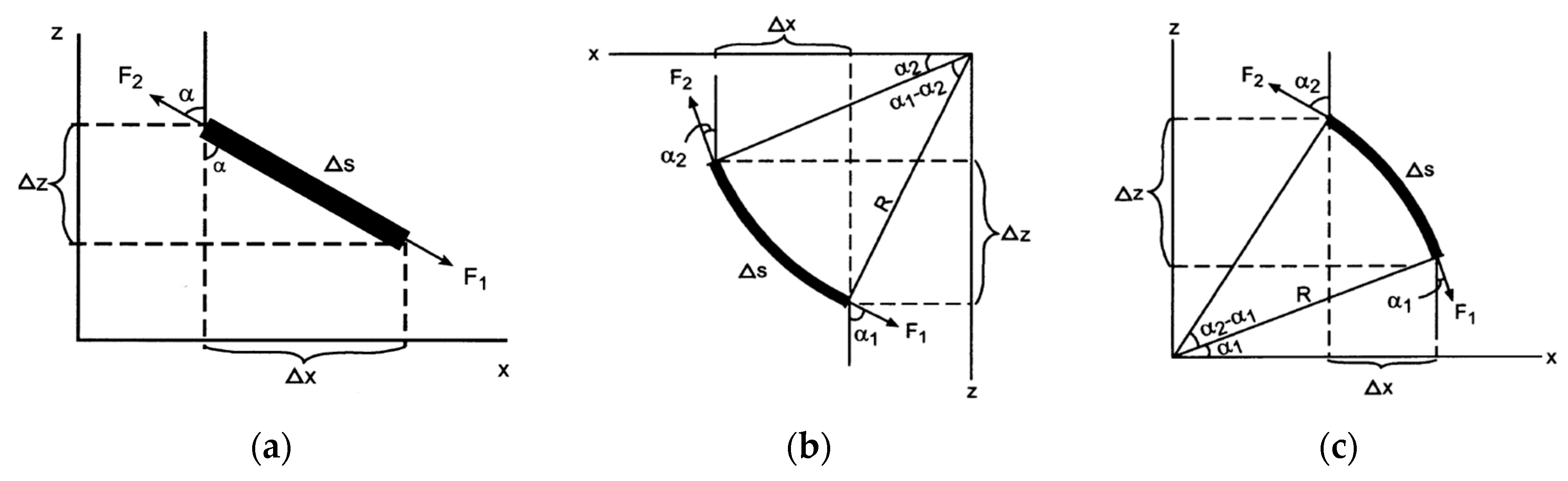
2.4.1. Heat Sources Induced by Mechanical Friction

(1) Heat source generated by friction at the drill bit
Using different types of drill bits for different categories of formations, the friction at the drill bit varied as well. Nguyen [25] and Warrant [52] presented the following function to estimate the heat source generated by friction at the drill bit:
q = 1 J ( 1 η ) ( W O B R O P + 2 π ω T b i t )  
where J is Joule’s constant, which is unity when both sides of Equation (22) are in a consistent unit system; η is the drill bit efficiency of the portion of work used for penetration; WOB is the weight on the bit; ROP is the rate of penetration; ω is rotary speed, RPS; Tbit is the torque on the bit.
(2) Heat source generated by friction between drill pipe and wellbore
● Vertical Hole
In drilling in vertical sections, we assumed that the drill pipes do not come into contact with the wellbore wall. Thus, friction between the drill pipe and wellbore wall was zero, and there was no heat source produced along vertical sections.
● Curved Hole (Built-Up or Drop-Off Section)
Aadnøy and Andersen [53] defined the drag forces and torques under drilling conditions in various well segments (shown in Figure 3), including pulling up and lowering down drill pipes.
(a)
Drop-off section
When pulling up drill pipes, the force at the upper side of each section was:
F 2 = F 1 e μ ( α 2 α 1 ) + w R 1 + μ 2 [ ( 1 μ 2 ) ( s i n α 2 e μ ( α 2 α 1 ) s i n α 1 ) 2 μ ( c o s α 2 e μ ( α 2 α 1 ) c o s α 1 ) ]  
When lowering down the drill pipe, the force at the upper side was:
F 2 = F 1 e μ ( α 2 α 1 ) + w R [ s i n α 2 e μ ( α 2 α 1 ) s i n α 1 ]  
The torque was given by:
T = μ r [ ( F 1 + w R s i n α 1 ) | α 2 α 1 | 2 w R ( c o s α 2 c o s α 1 ) ]  
(b)
Built-up section
When pulling up drill pipes:
F 2 = F 1 e μ ( α 2 α 1 ) w R [ s i n α 2 e μ ( α 2 α 1 ) s i n α 1 ]  
When lowering down drill pipes:
F 2 = F 1 e μ ( α 2 α 1 ) w R 1 + μ 2 [ ( 1 μ 2 ) ( s i n α 2 e μ ( α 2 α 1 ) s i n α 1 ) 2 μ ( c o s α 2 e μ ( α 2 α 1 ) c o s α 1 ) ]  
The torque was:
T = μ r [ ( F 1 + w R s i n α 1 ) | α 2 α 1 | + 2 w R ( c o s α 2 c o s α 1 ) ]  
(c)
Straight inclined hole
For tangential sections, the inclination of the wellbore was constant and drill pipes were laid down on the low side of the borehole. The drag force at the upper side of each wellbore section was
F 2 = F 1 + w Δ s ( c o s α ± μ s i n α )  
where “+” was for pulling-up processes, and “−” was for lowering-down processes. The torque was
T = μ r w Δ s s i n α  
It was noticeable that the drill pipes were always immerged in drilling fluids; therefore, buoyancy should be taken into consideration. The parameter w is the buoyed pipe weight and computed as:
w = β w d  
where wd is the weight of the drill pipe in air, and β is the buoyancy factor. Aadnoy [54] defined it as follows: (a) When the drilling fluid density in drill pipes was not equal to that in the annulus, β = 1 − (ρoAoρiAi)/[ρpipe(AoAi)], where ρ is the density, A is the cross-sectional area. The subscripts o, i, and pipe represented the fluid in the annulus, fluid in the drill pipes, and drill pipes themselves, respectively; (b) When the drilling fluid density in drill pipes equaled that in the annulus, then:
β = 1 ρ o / ρ p i p e  
Using Equations (23)–(32), the torque in drill pipes can be calculated because of the friction between the drill pipe and wellbore wall. The heat quantity produced by the drill pipe per unit time can be computed as well [55], as follows:
Q f r i c t i o n = 2 π R P S T  
where RPS denotes rotations per second, r/s. Equation (33) was used to estimate the heat source of friction between the drill pipe and wellbore wall. After discretizing the entire drill pipe into a number of sections along the direction of the well depth, the total heat source can be computed by adding the heat source at each section—from the first section, at the well bottom, to the last section, at the well head. Moreover, the friction factor, μ, highly depended on the roughness of contact surfaces, properties of the drilling fluid, and temperature and pressure conditions. Craig [56] analyzed 33 wells in a Norwegian platform and reported that μ = 0.24 was the most applicable friction factor for all types of wells, and the condition of the well trajectory had an insignificant effect on the friction factor. Table 1 lists the friction factors between the drill pipes and wellbore wall using different drilling fluids, as reported by Samuel [57].

2.4.2. Heat Sources of Circulating Pressure Losses in Dill Pipe, Annulus, and Drill Bit

The drilling fluid flowed in drill pipes and the annulus gap between the outer wall of drill pipes and wellbore wall. This resulted in pressure drops because of the friction between the fluid and solid. This energy was eventually converted to heat sources along the well pipes. Keller [12] applied an empirical method to estimate heat sources during drilling procedures: 20% of the drilling pump hydraulic power loses in drill pipes, 8.5% loses in the annulus, and 70% loses at the drill bit. Based on the assumption that flow was turbulent in the drill pipes and drill bit, and laminar flow in the annulus space, the properties of the drilling fluid were in accord with those of the power-law fluid. Marshall and Bentsen [13] derived the following formulas to calculate circulating pressure drops:
  • Drill String:
    Δ P d = 2 f ρ V 2 L D g c 1 f = 4.07 n log r × 10 3 ε + 6.0 2.65 n  
  • Drill Bit:
    Δ P b = ρ 2 g ( q 0.95 A n )  
  • Annulus:
    Δ P a = 2 K L ( r o r i ) g c [ 2 ( n + 1 ) q n π ( r o + r i ) ( r o r i ) 2 ] n  
where f is the Fanning friction factor, D is the inner diameter of the drill pipe, gc is a unit conversion factor (127.094 × 10⁶ m/h2), g is the acceleration of gravity, q is the pump displacement, An is the area of bit nozzles, n is the fluid flow behavior index, K the fluid consistency index (kg/h2−n·m), ro and ri are outer and inner diameters of the annulus, respectively, and L is length of the drill pipe and annulus.
In this study, the method of Reed and Pilehvari [58], and Kelessidis [59] for non-Newtonian fluids subjected to the Herschel-Bulkley model was used to compute pressure drops in the drill pipe and annulus. Moreover, the effects of the rotary drill pipe with its eccentricity on the pressure drop in the annulus were considered.
The above expressions presented by Marshall and Bentsen [13] did not consider the effects of rotation and eccentricity of the drill pipes. In this study, only the effects of these two on the pressure drop in the annulus were investigated; however, it supposed that they have no influence on the drill pipe. As for non-Newtonian fluids, Cartalos and Dupuis [60] presented a ratio of the pressure drop in the annulus with a rotary inner pipe to the pressure drop with a stationary inner pipe, as shown below:
R r o t = ( d P / d L ) r o t ( d P / d L ) n o n r o t = [ 1 + 3 2 ( S o ( z ) d ) 2 ] 1 / 2  
where d = rori, So(z) is the amplitude of the inner pipe at a certain depth and replaceable with a mean value, Savg. Thus, the mean eccentricity is eavg = Savg/d, which is applicable to the whole well.
Through numerical stimulation, Ooms and Kampman–Reinhartz [61] studied the rotation of the inner pipe in relation to the pressure drop in the annulus when eccentricity was present with the drop during drilling in a slim borehole. Under a low rotary speed, they used a perturbation calculation to derive a formula for estimating the rotation in relation to pressure drop. The correction coefficient is
R r o t = [ 1 + 3 2 e 2 ] × [ 1 + 3 2 e 2 + 1 739200 δ 2 T a 2 ε 2 ( 2 + ε 2 ) 2 f ( e ) ] 1 f ( e ) = 13120 + 38112 e 2 10608 e 4 33062 e 6 1221 e 8
where δ = RoRi is the annulus space gap, e is the dimensionless eccentricity, e = dc/δ; dc is the distance between the center points of drillpipe and wellbore, and Ta is the Taylor number based on the outer radius of the annulus, i.e., Ta = ρωRo(RoRi)/μ. They reported that only when δεTa is much less than 1 can Equation (38) be applied. When the Taylor number was high, numerical simulation should be employed.
Ahmed [62] presented a fitted formula for the rotation correction coefficient based on experimental data derived from the yield-power-law drilling fluid. The coefficient was named PLR, defined as the ratio of the pressure drop in the annulus with a rotary inner pipe to that in the annulus with a stationary pipe:
R r o t = 0.36 × ( 13.5 + τ y ρ V a 2 ) 0.428 × e a v g 0.158 × n 0.054 × T a 0.0319 × R e e f f 0.042 × k ( 1 k 1 ) 0.0152  
where T a = D i ( D o D i ) 3 16 ( ρ ω μ a p p ) 2 ; R e e f f = 8 ρ V a 2 τ w , l a m ; k = D i D o ; μ a p p = τ y γ ˙ + K γ ˙ n 1 .
In the study of Anifowoshe and Osisanya [63], γ ˙ = γ ˙ a 2 + γ ˙ θ 2 = ( 12 V a ( 2 n + 1 ) D h 3 n ) 2 + ( ω D i D h ) 2 , where τy and n are the fluid yield stress and flow behavior index for Herschel-Bulkley fluid, respectively; Va is the mean velocity of the fluid in annulus; k is the ratio of the inner diameter to the outer diameter of the annulus; μapp is the apparent viscosity; γ ˙ is the resultant shearing rate, combining axial and tangential velocities; τw,lam is the mean shear stress on the wall. Ahmed [62] indicated that the above formula was applicable when the mean eccentricity, eavg, was between 0.5 and 1.0, the effective Reynolds number, Reeff, ranged from 721 to 2397, and Ta0.5 was between 479 and 1602.
Haciislamoglu and Langlinais [64], and Haciislamoglu [65] introduced two correction coefficients to take into account the effects of rotary and eccentric drill pipes for calculating the pressure drop when yield-power-law drilling fluid flowed through the annulus.
Laminar regime:
R e c c = ( d P / d L ) e c c ( d P / d L ) c o n = 1 0.072 e n ( D i D o ) 0.8454 1.5 e 2 n ( D i D o ) 0.1852 + 0.96 e 3 n ( D i D o ) 0.2527  
Turbulent regime:
R e c c = ( d P / d L ) e c c ( d P / d L ) c o n = 1 0.048 e n ( D i D o ) 0.8454 2 3 e 2 n ( D i D o ) 0.1852 + 0.285 e 3 n ( D i D o ) 0.2527  
Haciislamoglu and Langlinais 64 stated that the two expressions were valid when 0 ≤ e ≤ 0.95, 0.3 ≤ Di/Do ≤ 0.9, 0.4 ≤ n ≤ 1.0. Here, the eccentricity is equal to 0 for vertical well segments (concentric), 0.62emax for inclined well segments (linearly eccentric), and 1 for horizontal well segments (completely eccentric). Pilehvari and Serth 66 modified the above formula for the laminar regime by replacing e/n with e∙n:
R e c c = 1 0.1019 e n ( D i D o ) 0.4675 1.6152 e 2 n 0.085 ( D i D o ) 0.7875 + 1.1434 e 3 n 0.0547 ( D i D o ) 1.1655  
The application range of n was extended to 0.2 ≤ n ≤ 1.0, the scope of the ratio Di/Do became 0.2 ≤ Di/Do ≤ 0.8, and the range of eccentricity, e, was unchanged. Using the modified expression, Recc is 1 as n → 0, instead of Recc −∞. All the requirements in the abovementioned new formula can be satisfied under all practical conditions in drilling operations. If the pressure drop in a concentric annulus was determined, then the correction coefficients can be used to take into account the effects of rotation and eccentricity of drill pipes, and the effects on pressure drop can finally be reflected in different wellbore temperature profiles.

3. Analysis of Wellbore Temperature Behavior during Deep Horizontal Well Drilling

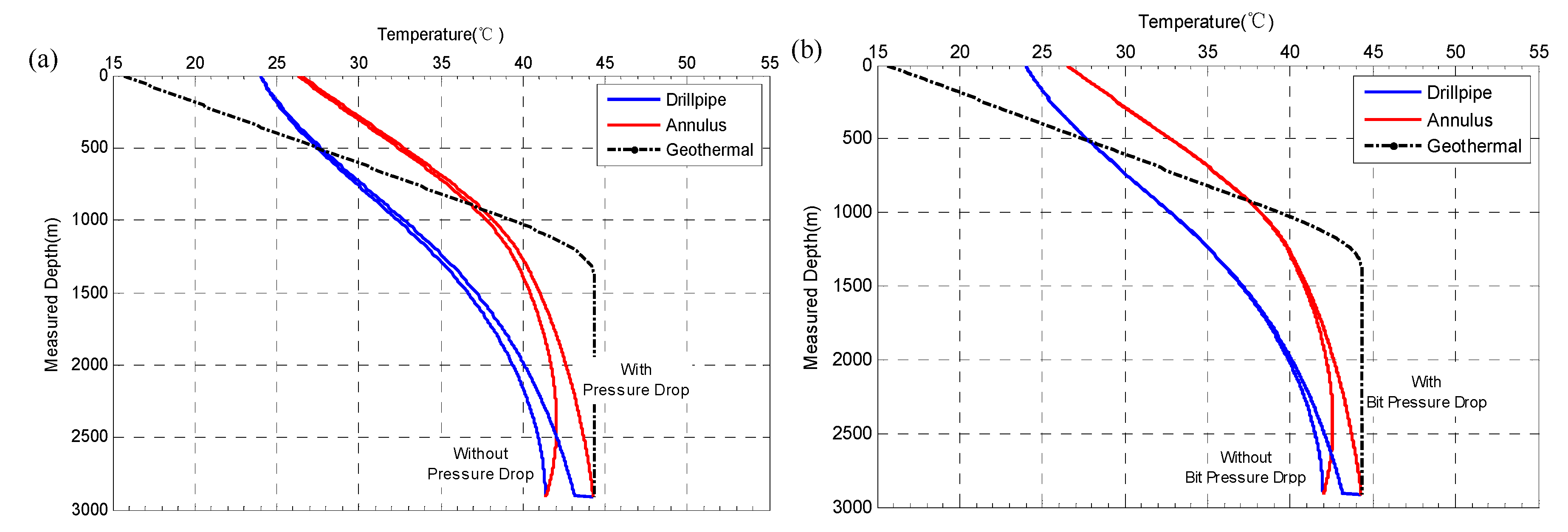
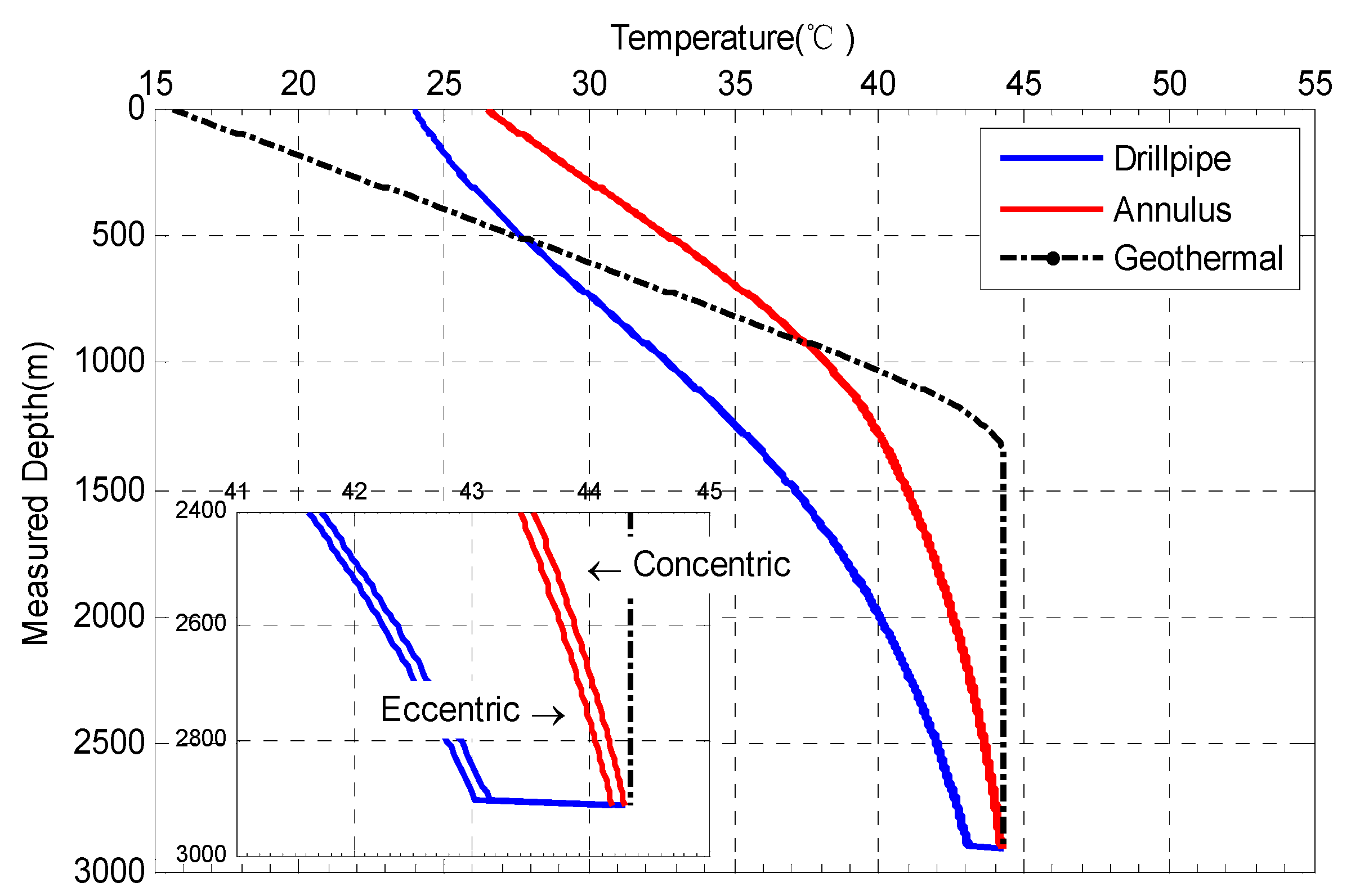
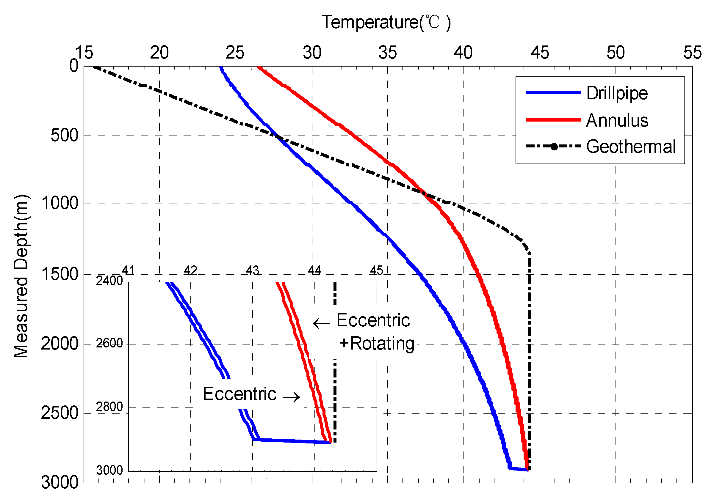
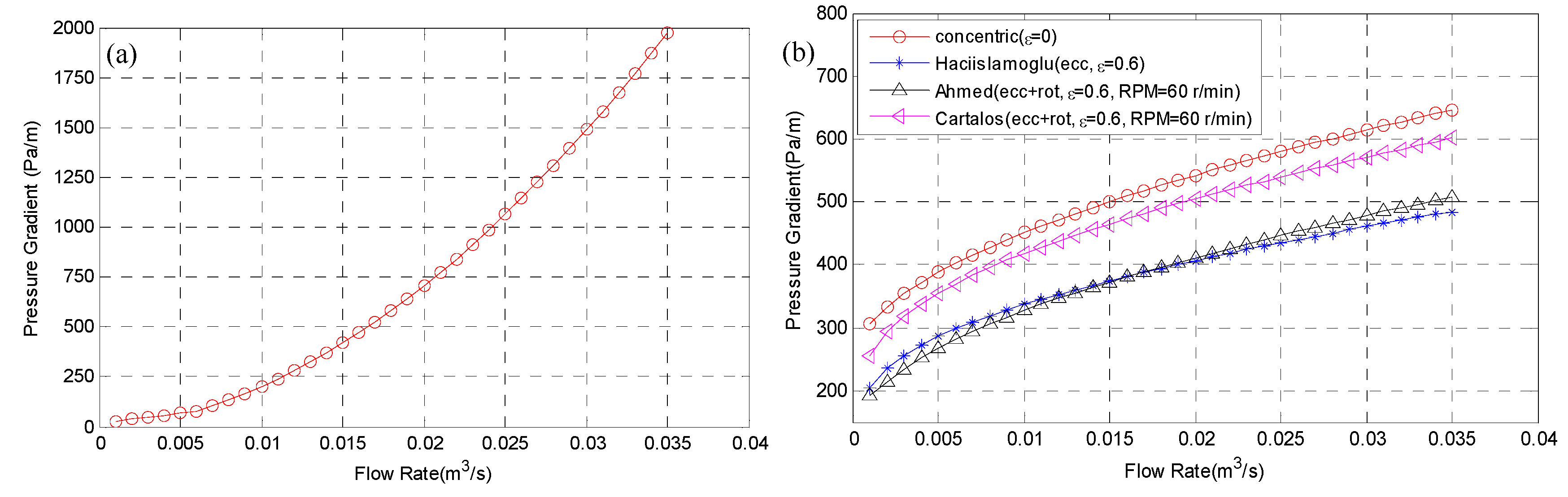
3.1. Influences of Circulating Pressure Drop under Various Rotation Rates and Eccentricities of Drill Pipes

As presented in Section 2.4.2, the pressure drop in the annuli of drill pipes can be computed. Accordingly, it can be transferred to heat sources, which contributed to temperature fluctuations along the wellbore. In this study, we assumed that all the heat generated within the drill pipes flowed with the drilling fluid in the drill pipes, and all the heat produced at the drill bit and annulus was transferred to the drilling fluid in the annulus. Firstly, the pressure drops in the drill pipe and annulus using the input parameters summarized in Table A1 in this study were calculated.
As shown in Figure 4, both pressure drops in the drill pipe and annulus increased with the increase in flow rate, which meant more heat was produced because of the hydraulic friction between the solid and fluid regions. In addition, when the eccentricity increased, pressure decreased. Furthermore, when an inner drill pipe rotated, the pressure drop in the annulus was higher than that with a stationary one (notice that in Figure 4b that Ahmed’s fitting expression did not conform to this law because it was not applicable when the flow rate was low).
Therefore, it was evident that the eccentricity of the inner drill pipes led to a decline in the pressure drop in the annulus, whereas the increase in rotatory speed produced reversed results. Based on input data in this study, the formula derived by Cartalos and Dupuis [60] was involved in the flow analysis.
According to the calculation procedure shown in Figure A4, the temperature profiles, considering drill pipe rotations, and hydraulic and mechanical frictions were obtainable. In Figure 5a, when the effect of the circulating pressure drop was considered, the temperature along the wellbore was higher than that when the pressure drop was neglected. The temperature difference, ΔT, tended to increase with increasing well depth and reached its maximum at the borehole bottom with the value ΔTa ≈ 3 °C. Moreover, the phenomenon, in which the maximum temperature along the wellbore was found at a certain distance from the borehole bottom, which was mentioned in a previous research on the temperature of vertical wellbores, occurred here as well when the effect of the circulating pressure drop was excluded. On the other hand, when the effect of the pressure drop was considered, the phenomenon disappeared. Meanwhile, temperature spurts occurred at the well bottom because of the substantial amount of hydraulic mechanical energy loss as the drilling fluid flowed through the bit nozzles. Figure 5b compares the temperature profile when only the pressure drop at the drill bit was taken into account and when pressure drop was neglected. However, a temperature difference of ΔTa ≈ 2 °C, which exhibited a high influence of the pressure drop on the drill bit, still remained.
According to Figure 6 and Figure 7, the eccentricity and rotation of drill pipes had insignificant effects on the temperature distribution along wellbore. When the eccentricities for the vertical, inclined, and horizontal sections were set to e = 0.6, e = 0.62, and e = 1, respectively, and the magnitude of revolutions per minute (RPM) of drill pipes was 100 r/min, the temperature difference at the wellbore bottom was only approximately 0.2 °C, which was negligible.

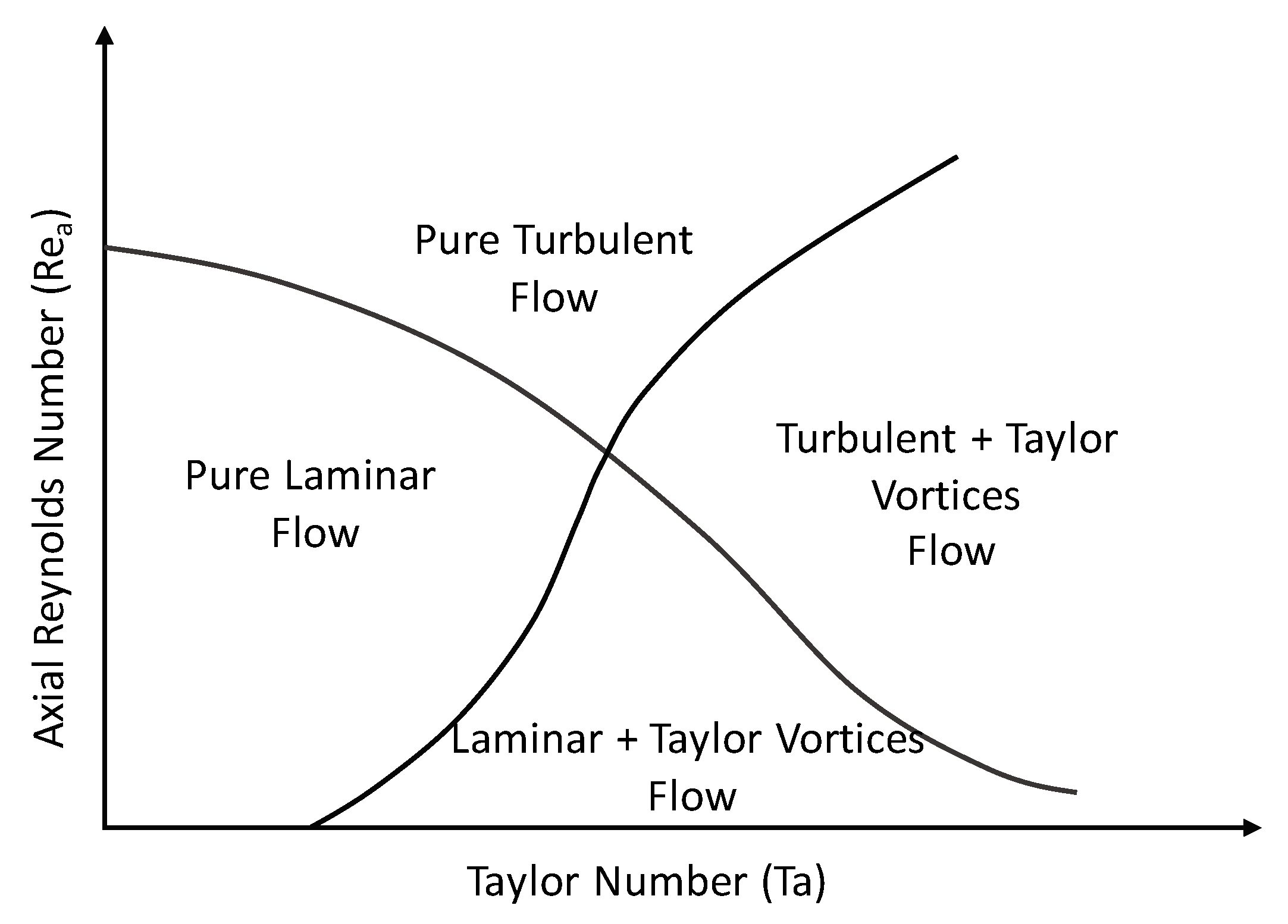
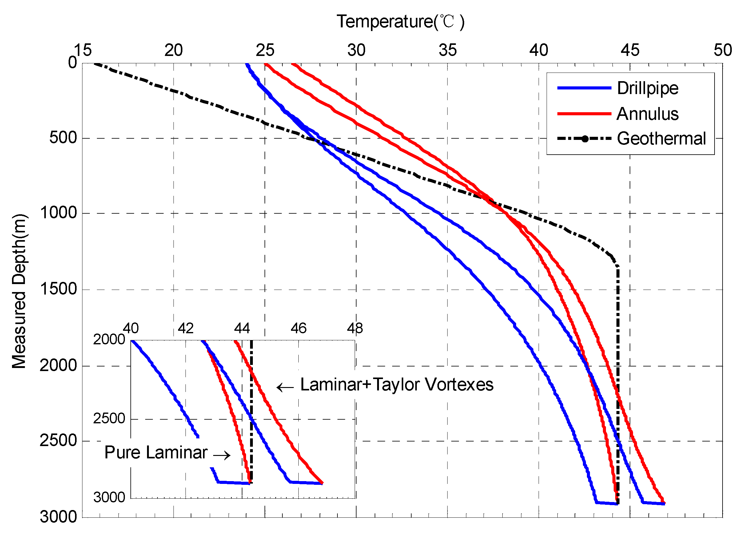
3.2. Influence of Nu with Taylor Vortex under Various Rotation Rates of Drill Pipe

For the annulus in which the inner wall was rotary, the Taylor vortex occurred under a certain condition; a phenomenon that had been validated by numerous studies [40,42,45,46]. In this regard, the drilling fluid flows in the annulus between the wellbore wall and drill pipe were no exception [32]. The appearance of Taylor vortices certainly made a difference on the heat transfer in the annulus. Thus, the consideration of the effect of the Taylor vortex was important in predicting the temperature profile during drilling procedures. In order to analyze the convective heat transfer coefficient, α = λeNu/Dh, an analysis of the variation of Nu was required while the Nu value was affected by the appearance of the Taylor vortex. In previous studies, the drilling fluid flow in the annulus was assumed to be laminar. However, with respect to the effect of drill pipe rotation, it was found that it triggered Taylor vortices under certain rotation rates of drill pipes. In this study, it was maintained that the flow regime in annulus with rotatory inner drill pipes was of the laminar + Taylor vortices mode instead of the pure laminar flow regime. Thus, the effect of the Taylor vortex on Nu and temperature distribution was analyzed. In this regard, we mainly used the expression of Simmers and Coney [48] to conduct our analysis.
Under the regime of laminar + Taylor vortices and axial flow rate unchanged, it can be observed in Figure 8 that the heat transfer in the wellbore was enhanced compared to that under the pure laminar regime. This was because under the laminar + Taylor vortices state, the temperature in the drill pipe was greater than that without Taylor vortices. Moreover, when Taylor vortices occurred, the temperature in the annulus at the upper wellbore section, where the temperature was higher than the geothermal temperature, was lower than that under the pure laminar state.
However, at the lower wellbore section, where the annulus temperature was lower than the geothermal temperature, the temperature was higher when Taylor vortices occurred. Figure 9a shows that when considering the Taylor vortex, the wellbore bottom temperature was always greater than that under the pure laminar state, and the expression provided by Seder and Tate [34] was used for the pure laminar regime to estimate the wellbore bottom temperature. The temperature remained unchanged when the rotation rate varied because Nu was merely influenced by the axial velocity. On the other hand, the bottom temperature increased as the rotation rate increased when the Taylor vortex emerged. This was because Nu was simultaneously affected by the rotation and axial flow rates. As seen in Figure 9b, the variation of the wellbore bottom temperature as Nu increased under the laminar + Taylor vortices regime was similar with the varying trend of the temperature in relation to the rotation rate shown in Figure 8a, where the wellbore bottom temperature increased as Nu increased. The phenomena revealed that Taylor vortices considerably intensified the heat transfer in the wellbore.

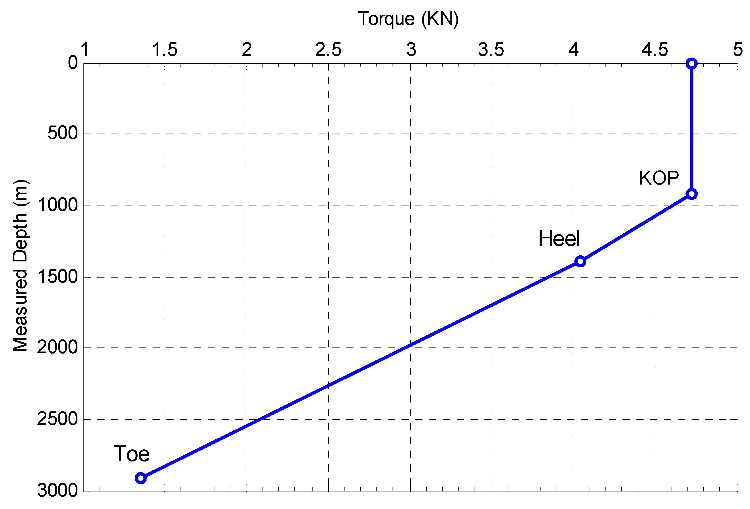
3.3. The Influence of Mechanical Friction under Various Rotation Rates of the Drill Pipe

In the drilling procedure, the drill pipes always had to rotate at high speeds in order to drive the drill bit to break the rocks. Hence, continuous contact and friction between the rock and drill bit, as well as with the drill pipes was inevitable. Therefore, as a result of mechanical friction, a substantial amount of heat was produced and the drilling fluid was gradually heated. In this study, we firstly computed the torque distribution (shown in Figure 10) along all drill pipes and drill bit according to studies conducted by Aadnøy and Andersen [53], and Warrant [52], and thereafter obtained the heat quantity in each small segment.
Evidently, the heat quantity was from the inner heat source because of mechanical friction. In the discussion in this section, it was assumed that all the heat generated by mechanical friction at the drilling pipes and drill bit were absorbed by the drilling fluid in the annulus.
The wellbore temperature distribution in the annulus under pure laminar conditions is plotted in Figure 11. It can be seen from Figure 11a that the temperature in the drill pipe and annulus was greater when mechanical frictions of the drill bit and drill pipes were considered than when they were neglected. As the depth of the well increased, the temperature difference between the two conditions increased and peaked at the wellbore bottom. In this calculation example, when the rotation speed was 100 r/min, the annulus temperature difference with and without mechanical friction at the bottom of the well was 8.4 °C. When friction was not considered, the bottom temperature increased by 20.26%. Therefore, mechanical frictions along the wellbore had a considerable influence on the temperature at the wellbore bottom. When the effects of frictional heat at the drill bit were separately investigated, it can be seen from Figure 11b that when only the mechanical friction on the outer wall of drill pipes was considered, the wellbore bottom temperature was approximately 2 °C lower than the temperature at which the drill bit friction was considered. Thus, under this condition, the change in the bottom hole temperature caused by friction at the drill bit was approximately 25.5% of the total temperature difference. In addition, it can be observed from Figure 11b that when the frictional heat source at the drill bit was considered, there was a sudden increase in temperature as the drilling fluid flowed into the annulus from the drill pipes at the wellbore bottom, and that this temperature variation only affected a limited distance above the drill bit. Evidently, the temperature distribution was not affected by heat sources produced at the drill bit beyond a certain distance above it. With reference to Figure 5b and Figure 11b, if the heat source at the drill bit was not taken into consideration, then, there was a temperature increase as the fluid flowed upwards through the annulus. The highest temperature in the annulus occurred at a certain distance from the wellbore bottom. However, when the influence of the heat source at the drill bit was considered, the phenomenon of temperature inversion mentioned by Kabir and Hasan [7] reduced or completely disappeared. A noteworthy difference between the temperature profile in the vertical well and bottom hole of the horizontal well was that when the heat source term was taken into account, the temperature in the latter may be greater than the original geothermal temperature. It can be seen in Figure 11 that, overall, the annulus temperature was higher than the original formation temperature when frictional heat sources were included.
The rotation rate of drill pipes affected the amount of heat generated during drilling processes. In Figure 12, without considering the effect of rotation on the convection heat transfer, the red line with circular markers and blue line with triangular markers show the temperature variations at the wellbore bottom when the heat source at the drill bit was taken into account and excluded, respectively. In both cases, it was evident that the wellbore bottom temperature in the annulus increased linearly as the rotational speed of drill pipes increased. On the other hand, if the effect of rotation on heat transfer was considered, this transfer increased as the rotation speed increased, but the magnitude of increase gradually became smaller.
A significant difference was observed among the temperature profiles when the effects of drill pipe rotation, pressure drops in the drill pipe and annulus because of hydraulic frictions, and heat sources derived from mechanical frictions were simultaneously considered and when they were neglected. The temperature difference in the annulus between the two conditions at the wellbore bottom reached up to 16 °C, which was 38% higher than the temperature when all effects were considered. Furthermore, as can be seen from Figure 13, the outlet temperature of the drilling fluid at the wellhead was only approximately 1 °C. Thus, although there was no noticeable temperature difference detected at the ground surface when computed under the aforementioned two conditions, there can be a significant temperature difference when depth increased, particularly at the wellbore bottom. In conclusion, the effects of drill pipe rotation, and hydraulic and mechanical frictions cannot be ignored in the estimation of temperature distribution in the entire horizontal well drilling process.

4. Conclusions

(1)
The pressure drops in drill pipes and annuli during horizontal well drilling had negligible effects on temperature distributions. Consequently, it was more reasonable to take into consideration the pressure drop at the drill bit. When all pressure drops were considered, the temperature difference at the wellbore bottom was 3 °C. However, if the pressure drop at the drill bit was ignored but pressure drops in the drill pipe and annulus were considered, the difference is still 2 °C. But for the pressure drop influenced by drill pipe rotation and eccentricity, it only leads to 0.2 °C difference in bottom hole temperature, which can reasonably be neglected.
(2)
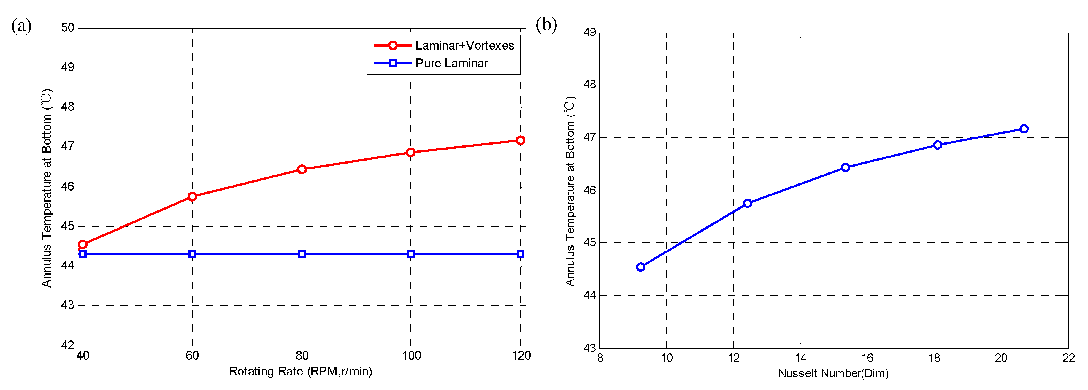
When the effect of drill pipe rotation on convection heat transfer in the annulus was considered, the occurrence of the Taylor vortex enhanced the heat transfer process. Compared to the heat transfer under the pure laminar regime, the temperature in the upper annulus was lower than that without the consideration of the effect of the drill pipe rotation, whereas the temperature in the lower annulus was greater.
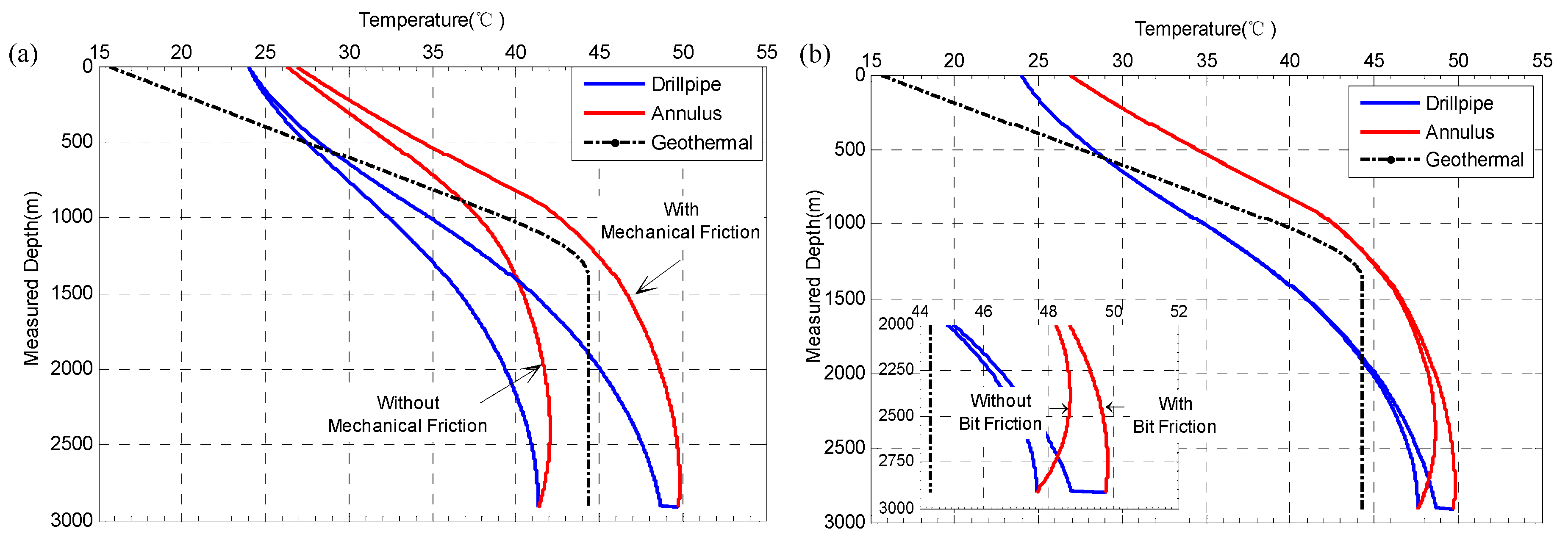
(3)
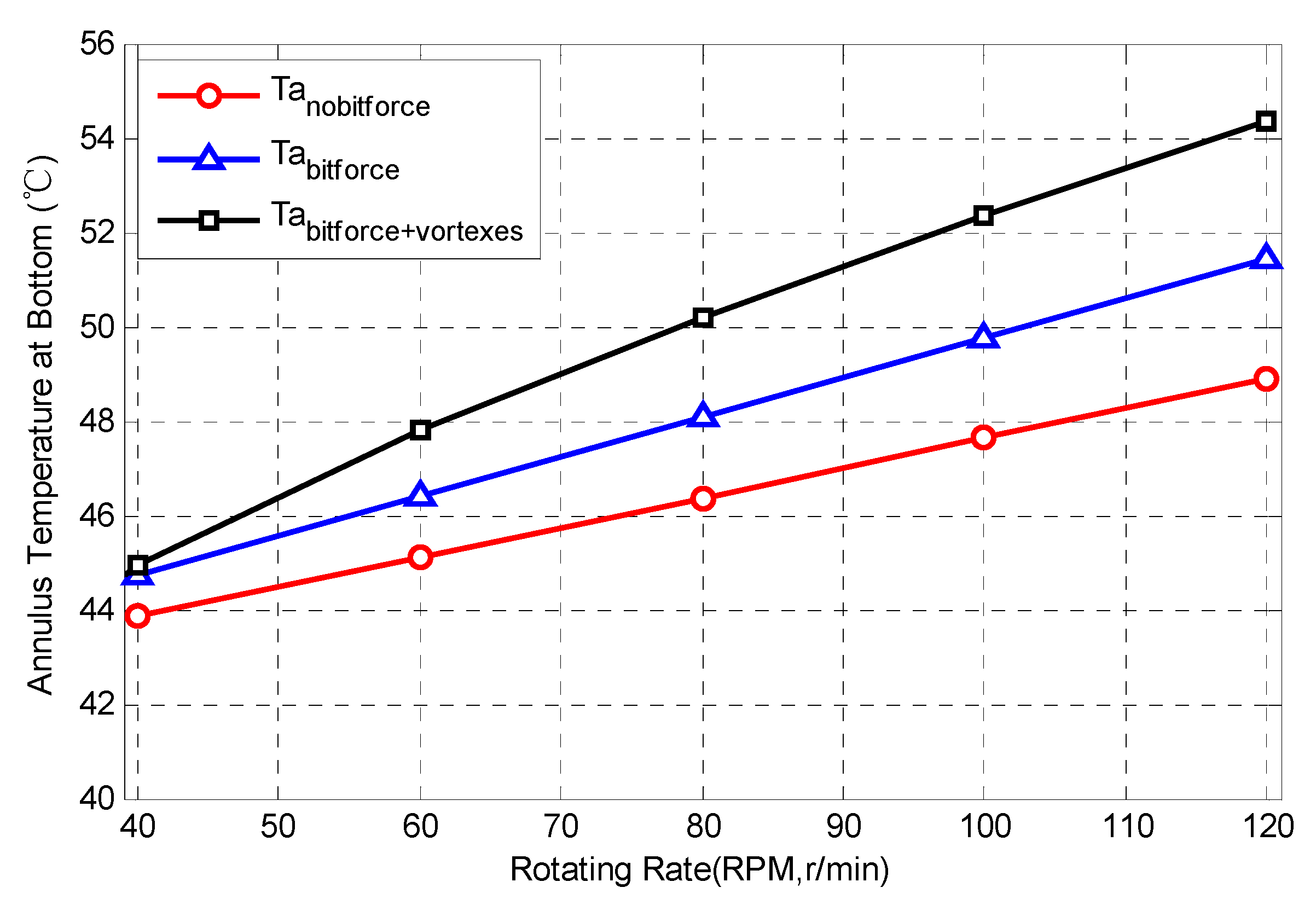
The mechanical friction at the drill bit and drill pipes had a great influence on the wellbore temperature. This effect increased as the rotation rate increased. Hence, the effect of mechanical friction cannot be ignored. When RPM = 100 r/min, the annulus temperature difference at the wellbore bottom between the conditions where mechanical friction was considered and neglected reached up to 8 °C, which was a 19% increase.
(4)
The annulus temperature difference at the wellbore bottom between the conditions in which all effects, including drill pipe rotation, and hydraulic and mechanical frictions, were considered and neglected reached up to 16 °C, which was approximately a 38% increase. Moreover, it was possible for the temperature at the horizontal section to be greater than the original geothermal temperature when the abovementioned effects were taken into consideration.
The conclusions above indicate that the heat sources generated from frictions have a strong impact on the temperature profile along wellbore, meanwhile, the rotation of drill pipes also make a distinct difference in heat transfer in the annulus. Some appropriate on-site countermeasures should be applied to reduce the bad effects of high temperature conditions at bottom hole of deep wells, for example, improving the lubricity and rheology of drilling fluid to reduce the mechanical and hydraulic frictions; strictly controlling the dogleg severity and using the rotary steering drilling tools to achieve precise control of wellbore trajectory; and the combined drilling technology is also beneficial to reduce the mechanical frictions; moreover, using the drilling fluid with stability in high temperature conditions when drilling extended long horizontal wells.
In the end, besides what we discussed in this paper, there are still many remaining issues we will investigate in the following work. Such as the effect degree of casing program on the heat transfer procedures during drilling horizontal wells, the thermal behaviors under a three-dimensional well trajectory, the variations of drilling fluid properties resulting from temperature changes, and the varying trends of heat transfer when the composition of drilling fluid is changed (the influx of formation fluids, the increase of cuttings concentration) should also be considered [15,67,68,69].

Author Contributions

Conceptualization, X.C. and S.H.; Data curation, Y.C., M.T. and R.J.; Formal analysis, X.C. and L.W.; Funding acquisition, Y.G., S.H. and L.W.; Investigation, Y.G.; Methodology, J.Z. and S.H.; Project administration, Y.G., S.H. and L.W.; Resources, Y.G. and L.W.; Software, J.Z.; Supervision, X.C. and S.H.; Validation, X.C., J.Z., S.H. and M.T.; Writing—original draft, X.C., J.Z., Y.C. and R.J.; Writing—review & editing, X.C., J.Z. and S.H.

Funding

The research was funded by the National Natural Science Foundation of China, grant numbers: 51574218, 51774247, 51474186 and 51574202; the project of the 12th Five-Year Plan of China, grant number: 2011ZX05045-03-01WX; the National Science and Technology Major Project of China (Nos. 2016ZX05060-004 and 2017ZX05036-003); Strategic Priority Research Program of the Chinese Academy of Sciences (No. XDB10040200); the Open Fund of the State Key Laboratory of Oil and Gas Reservoir Geology and Exploitation (Southwest Petroleum University), grant number: PLN0015; the Scientific Research Starting Project of Southwest Petroleum University, grant number: 2017QHZ001.

Conflicts of Interest

The authors declare no conflict of interest.

Nomenclature

cd, cl, crheat capacity of drill pipe, mud and formation, J/(kg·°C);
Ddi, Ddo, Dwinner and outer diameters of drillpipes, the wellbore diameter, respectively, m;
Dn1, Dn2, Dn3diameters of three nozzles at drill bit, mm;
DHhydraulic diameter, m;
dP/dLpressure drop gradient along drill pipe, Pa/m;
eeccentricity of drill pipe, -;
F1, F2the force at the lower and upper end of a drillpipe segment, respectively, N;
Fbitbit efficiency, -;
fhydraulic friction factor, -;
fnnozzle orifice coefficient, -
GTgeothermal gradient, °C/m;
Ha certain well depth, m;
Hheelmeasured depth of the heel of horizontal section, m;
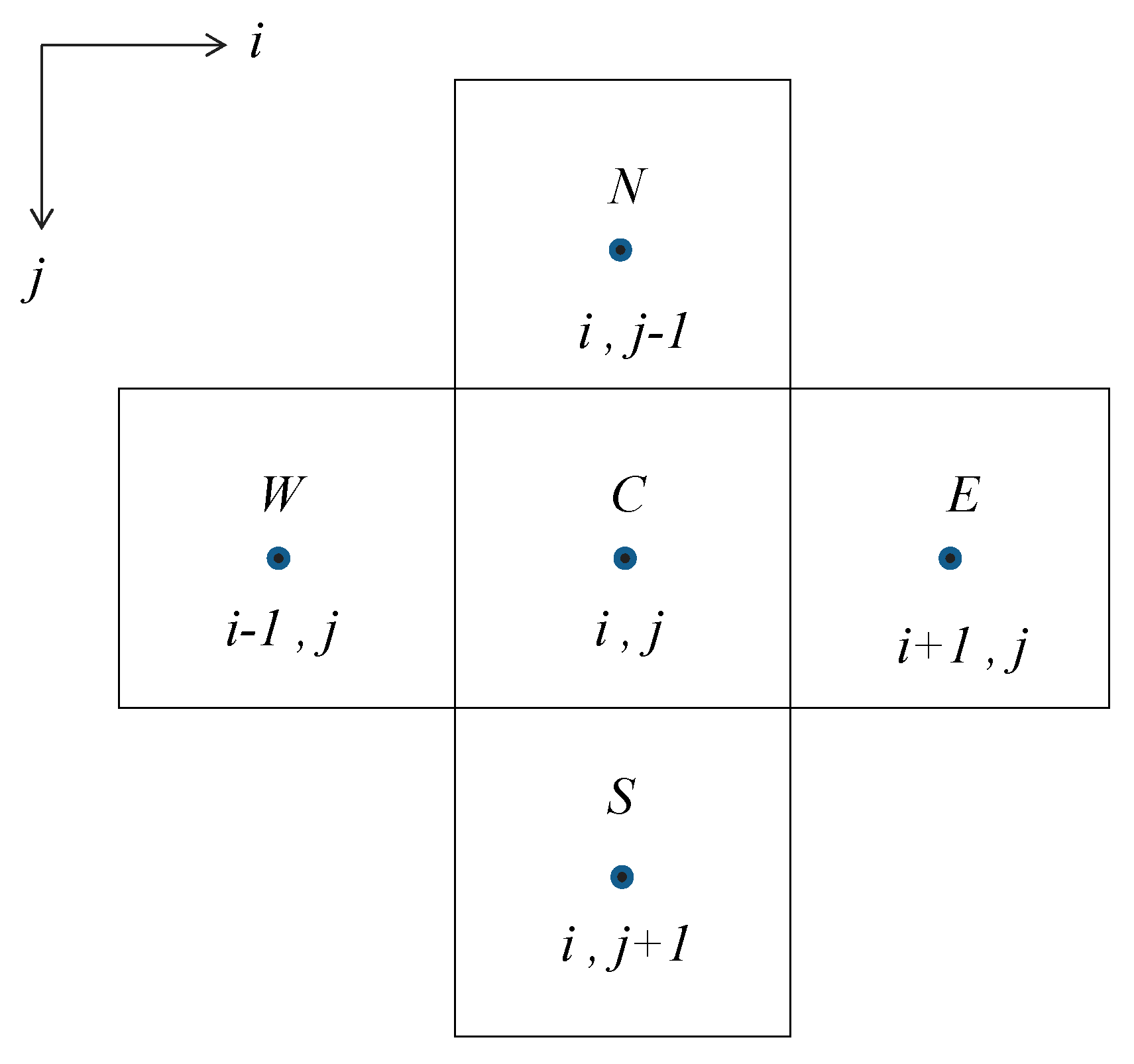
ithe number of radial grid layer, -;
jthe number of axial grid layer, -;
Kfluid consistency index, Pa·sn;
NuNusselt number, dimensionless;
nfluid flow behavior index, -; or the time step in the differential equations;
PrPrandtl number, dimensionless;
Qi, Qoheat sources within the drill pipe and that within annulus, J;
qcirculating rate, m3/h;
Rreservoir radius, m;
Rbradius of built-up section, m;
Reccratio of pressure drop along eccentric annulus to that along concentric annulus, -;
Rrotratio of pressure drop in annulus with a rotating drill pipe to that in annulus with a stationary drill pipe, -;
ReReynolds number, dimensionless;
Reaaxial Reynolds number, dimensionless;
Reeffeffective Reynolds number, dimensionless;
r1, r2, r3inner and outer radius of drillpipes, the wellbore radius, respectively, m;
Ttorque along wellbore, kN·m;
Ta, Ta*Taylor number, dimensionless;
Tbittorque on bit, kN·m;
Tin, Tsinlet and surface temperature, respectively, °C;
Tl, Td, Tla, Tr, Tbtemperature of mud in drill pipe, drill pipe, mud in annulus, formation and wellbore wall, respectively, °C;
tcirculating time, s;
w, wdweight of drill pipe per meter in mud and air, respectively, kN/m;
zthe measured depth of well, m;
Greek Letters
α1, α2inclination angle at the lower and upper end of a drill pipe segment, respectively, °;
αdi, αbconvective heat-transfer coefficient at the inner face of the drill pipe and the wellbore wall, respectively, W/(m2·°C);
βbuoyancy factor, -;
μmechanical friction factor (Equations (23)–(30)), -; or dynamic viscosity of mud (Equation (8); Equation (13)), Pa∙s;
ωrotary speed per minute, r/min;
ρd, ρl, ρrdensity of drill pipe, mud and formation rock, respectively, kg/m3;
δthe annulus space gap, m;
Δslength of a drill pipe segment, m;
λd, λl, λrthermal conductivity of drill pipe, mud and formation, respectively, W/(m·K);
τyfluid yield stress, Pa;
Abbreviations
KOPkick off point, m;
RPM, RPSrotary speed per minute/second, r/min or r/s;
ROPrate of penetration, m/h;
WOBweight on bit, kN;
W, C, E, N, Sthe name of grids, i.e., West(W), Center(C), East(E), North(N), South(S);

Appendix A

Appendix A.1. Discretization of Heat Transfer Model

In terms of the characters of absolute stability for the full implicit finite difference method, the first-order forward and central difference schemes were employed in the discretization of time and space, respectively.
As shown in Figure A1 and Figure A2, n denotes time step, i is the radial grid layer, and j is the axial grid layer. Therefore, the mathematical model can be discretized as that reported in [12,15].
Figure A1. Diagram of grid scheme.
Energies 11 02414 g0a1
Figure A2. The rule for naming grids.
Energies 11 02414 g0a2
(1)
Drilling fluid in drill pipe
c l ρ l q ( T 1 , j n + 1 T 1 , j 1 n + 1 Δ z j ) + α d i 2 π r 1 ( T 2 , j n + 1 T 1 , j n + 1 ) + Q i = c l ρ l π r 1 2 ( T 1 , j n + 1 T 1 , j n Δ t )  
(2)
Drill pipe
λ d 1 Δ z j ( T 2 , j + 1 n + 1 T 2 , j n + 1 Δ z j + 0.5 T 2 , j n + 1 T 2 , j 1 n + 1 Δ z j 0.5 ) + 2 r 1 α d i r 2 2 r 1 2 ( T 1 , j n + 1 T 2 , j n + 1 ) 2 r 2 α d o r 2 2 r 1 2 ( T 2 , j n + 1 T 3 , j n + 1 ) = c d ρ d ( T 2 , j n + 1 T 2 , j n Δ t )  
(3)
Drilling fluid in annulus
c l ρ l q ( T 3 , j n + 1 T 3 , j 1 n + 1 Δ z j ) + α d o 2 π r 2 ( T 2 , j n + 1 T 3 , j n + 1 ) α b 2 π r 3 ( T 3 , j n + 1 T 4 , j n + 1 ) + Q o = c l ρ l ( r 3 2 r 2 2 ) ( T 3 , j n + 1 T 3 , j n Δ t )  
(4)
Formation
α r b 2 e 2 x 1 Δ x j ( T i + 1 , j n + 1 T i , j n + 1 Δ x j + 0.5 T i , j n + 1 T i 1 , j n + 1 Δ x j 0.5 ) + α 1 Δ z j ( T i , j + 1 n + 1 T i , j n + 1 Δ z j + 0.5 T i , j n + 1 T i , j 1 n + 1 Δ z j 0.5 ) = T i , j n + 1 T i , j n Δ t  
(5)
Boundary and Initial conditions
  • Inlet condition: T 1 , 1 n = T i n
  • Temperatures at wellbore bottom: T 1 , j max n = T 2 , j max n = T 3 , j max n
  • Coupled condition at wellbore wall: α b ( T 4 , j n T 3 , j n ) = λ r T 5 , j n T 4 , j n r 4 r 3
  • Far field boundary: T , j n = T s u r f + G T j Δ z
  • Stratum holds the original temperature: T i , j | t = 0 = T s u r f + G T j Δ z
  • Drilling fluid in drill pipe: T 1 , j | t = 0 = T i n + G f j Δ z
  • Drilling fluid in annulus: T 1 , j | t = 0 = T o u t + G f j Δ z
If the grid number along the radial direction is iMAX, and that along the depth direction was jMAX, the sequence of all items in the discretized equations was rearranged according to Equation (A5). Thereafter, an equation set (iMAXjMAX × iMAXjMAX), shown as Equation (A6), was adopted to compute the temperature in the wellbore and surrounding rock. Because the coefficient matrix of the equation set was a large five-diagonal sparse matrix, the chasing method for the block tridiagonal matrix was employed to solve it.
W i , j T i 1 , j n + 1 + C i , j T i , j n + 1 + E i , j T i + 1 , j n + 1 + N i , j T i , j 1 n + 1 + S i , j T i , j + 1 n + 1 = B i , j  
The rule in naming the coefficients and grids is illustrated in Figure 3. The West (Wij, Ti−1,j), Centre (Cij, Ti,j), East (Eij, Ti+1,j), North (Nij, Ti,j−1), South (Sij, Ti,j+1). Equation (A5) can be rewritten into a matrix form:
  [ C E S W C E S W C E S W C E S N W C E N W C E N W C E N W C ]   ( i max j max × i max j max )     [ T 1 , 1 n + 1 T 2 , 1 n + 1 T i 1 , j n + 1 T i , j n + 1 T i , j n + 1 T i + 1 , j n + 1 T i max 1 , j max n + 1 T i max , j max n + 1 ]   ( i max j max × 1 ) = [ B 1 , 1 B 2 , 1 B i 1 , j B i , j B i , j B i + 1 , j B i max 1 , j max B i max , j max ] ( i max j max × 1 )
Based on Equation (A6), it was easy to solve the matrix by a series of iterations. However, three key parameters should be investigated: one is the convective heat transfer coefficient, αi (i = di, do or b), and the other two are heat sources Qi and Qo. In the following, the methods for determining them are discussed.

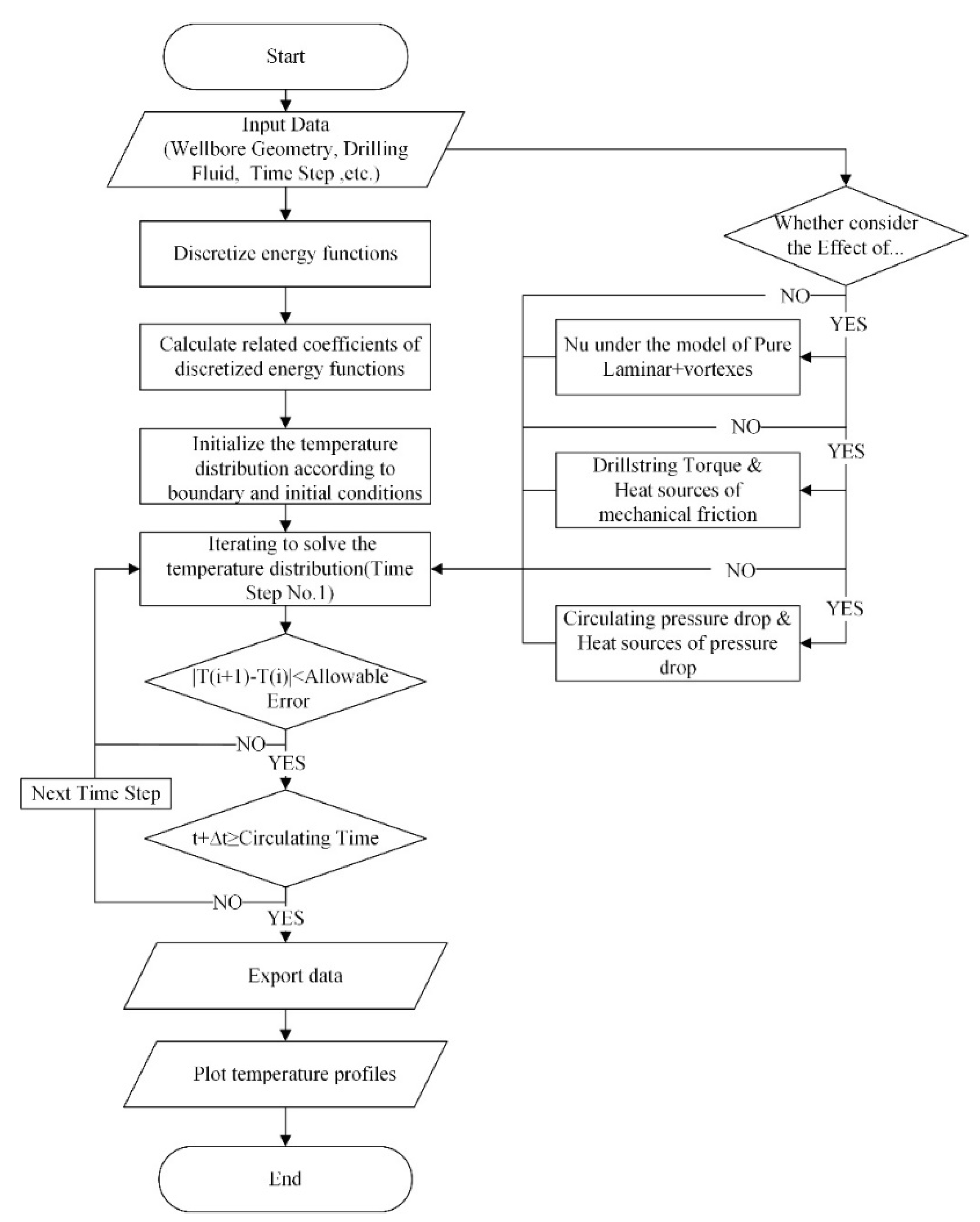
Appendix A.2. Input Data and Calculation Procedure

The input data summarized Table A1 for the case study were mainly referred from Nguyen [25,67]. The geometry parameters of the horizontal well employed in this study are in shown in Figure A3. In this study, all analyses were conducted on the basis of input data, unless otherwise noted. The calculation procedure is shown in Figure A4.
Figure A3. Well profile applied in this study.
Energies 11 02414 g0a3
Figure A4. Flowchart of calculation procedure.
Energies 11 02414 g0a4
Table A1. The input data for the case study in this paper.
ParametersValueUnitParametersValueUnit
Circulating time, t21,600sRotary speed, RPM100r/min
Reservoir radius, R3mTorque on bit, Tbit1.35kN·m
Kick off point, KOP914.4mInlet temperature, Tin23.89°C
Heel of horizontal section, Hheel1393.18mSurface temperature, Ts15.56°C
Radius of built-up section, Rb304.8mGeothermal gradient, GT0.0238°C/m
Diameter of Nozzle #1, Dn118mmMud thermal conductivity, λl1.73W/(m·K)
Diameter of Nozzle #2, Dn218mmFormation thermal conductivity, λr2.249W/(m·K)
Diameter of Nozzle #3, Dn316mmDrill pipe thermal conductivity, λd34.6W/(m·K)
Fluid yield stress, τy5.75PaMud heat capacity, cl1674.8J/(kg·°C)
Fluid consistency index, K0.3832Pa·snFormation heat capacity, cr837.4J/(kg·°C)
Fluid flow behavior index, n0.7-Drill pipe heat capacity, cd460.57J/(kg·°C)
Circulating rate, q47.696m3/hMud density, ρl1198kg/m3
Drill pipe inner diameter, Ddi0.101mDrill pipe density, ρd8000kg/m3
Drill pipe outer diameter, Ddo0.114mFormation density, ρr2645kg/m3
Wellbore diameter, Dw0.216mMechanical friction factor, μ0.2-
Weight of drill pipe per meter, wd0.186kN/mBit efficiency, Fbit0.8-
Rate of penetration, ROP14.4m/hNozzle orifice coefficient, fn0.95-
Weight on bit, WOB22.241kN

References

  1. Edwardson, M.J.; Girner, H.M.; Parkison, H.R.; Williams, C.D.; Matthews, C.S. Calculation of Formation Temperature Disturbances Caused by Mud Circulation. J. Pet. Technol. 1962, 14, 416–426. [Google Scholar] [CrossRef]
  2. Ramey, H.J.J. Wellbore Heat Transmission. J. Pet. Technol. 1962, 14, 427–435. [Google Scholar] [CrossRef]
  3. Holmes, C.S.; Swift, S.C. Calculation of Circulating Mud Temperatures. J. Pet. Technol. 1970, 22, 670–674. [Google Scholar] [CrossRef]
  4. Arnold, F.C. Temperature Variation in a Circulating Wellbore Fluid. J. Energy Resour. Technol. 1990, 112, 79–83. [Google Scholar] [CrossRef]
  5. Hasan, A.R.; Kabir, C.S. Heat Transfer during Two-Phase Flow in Wellbores; Part I—Formation Temperature. In Proceedings of the SPE Annual Technical Conference and Exhibition, Dallas, TX, USA, 6–9 October 1991. [Google Scholar] [CrossRef]
  6. Karstad, E.; Aadnoy, B.S. Analysis of Temperature Measurements during Drilling. In Proceedings of the SPE Annual Technical Conference and Exhibition, San Antonio, TX, USA, 5–8 October 1997. [Google Scholar] [CrossRef]
  7. Kabir, C.S.; Hasan, A.R.; Kouba, G.E.; Ameen, M. Determining Circulating Fluid Temperature in Drilling, Workover, and Well Control Operations. SPE Drill. Complet. 1996, 11, 74–79. [Google Scholar] [CrossRef]
  8. Aniket, A.; Pratap Singh, A.; Samuel, R. Analytical Model to Predict the Effect of Pipe Friction on Downhole Temperatures for Extended Reach Drilling (ERD). In Proceedings of the IADC/SPE Drilling Conference and Exhibition, San Diego, CA, USA, 6–8 March 2012. [Google Scholar] [CrossRef]
  9. Kumar, A.; Samuel, R. Analytical Model to Estimate the Downhole Temperatures for Casing while Drilling Operations. In Proceedings of the SPE Annual Technical Conference and Exhibition, San Antonio, TX, USA, 8–10 October 2012. [Google Scholar] [CrossRef]
  10. Livescu, S.; Wang, X. Analytical Downhole Temperature Model for Coiled Tubing Operations. In Proceedings of the SPE/ICoTA Coiled Tubing and Well Intervention Conference and Exhibition, The Woodlands, TX, USA, 25–26 March 2014. [Google Scholar] [CrossRef]
  11. Raymond, L.R. Temperature Distribution in a Circulating Drilling Fluid. J. Pet. Technol. 1969. [Google Scholar] [CrossRef]
  12. Keller, H.H.; Couch, E.J.; Berry, P.M. Temperature Distribution in Circulating Mud Columns. Soc. Pet. Eng. J. 1973, 13, 23–30. [Google Scholar] [CrossRef]
  13. Marshall, D.W.; Bentsen, R.G. A Computer Model to Determine the Temperature Distributions in a Wellbore. J. Can. Pet. Technol. 1982. [Google Scholar] [CrossRef]
  14. Song, X.; Guan, Z. Coupled modeling circulating temperature and pressure of gas–liquid two phase flow in deep water wells. J. Pet. Sci. Eng. 2012, 92–93, 124–131. [Google Scholar] [CrossRef]
  15. Yang, M.; Yingfeng, M.; Gao, L.; Li, Y.; Chen, Y.; Zhao, X.; Li, H. Estimation of Wellbore and Formation Temperatures during the Drilling Process under Lost Circulation Conditions. Math. Probl. Eng. 2013, 2013. [Google Scholar] [CrossRef]
  16. Gorman, J.M.; Abraham, J.P.; Sparrow, E.M. A novel, comprehensive numerical simulation for predicting temperatures within boreholes and the adjoining rock bed. Geothermics 2014, 50, 213–219. [Google Scholar] [CrossRef]
  17. Li, M.; Liu, G.; Li, J.; Zhang, T.; He, M. Thermal performance analysis of drilling horizontal wells in high temperature formations. Appl. Therm. Eng. 2015, 78, 217–227. [Google Scholar] [CrossRef]
  18. Bassam, A.; Santoyo, E.; Andaverde, J.; Hernández, J.A.; Espinoza-Ojeda, O.M. Estimation of static formation temperatures in geothermal wells by using an artificial neural network approach. Comput. Geosci. 2010, 36, 1191–1199. [Google Scholar] [CrossRef]
  19. Wu, B.; Zhang, X.; Jeffrey, R.G. A model for downhole fluid and rock temperature prediction during circulation. Geothermics 2014, 50, 202–212. [Google Scholar] [CrossRef]
  20. Siu, A.; Li, Y.; Nghlem, L.; Redford, D. Numerical Modelling of a Thermal Horizontal Well. In Annual Technical Meeting; Petroleum Society of Canada: Calgary, AB, Canada, 1990. [Google Scholar]
  21. Yoshioka, K.; Zhu, D.; Hill, A.D.; Dawkrajai, P.; Lake, L.W. A Comprehensive Model of Temperature Behavior in a Horizontal Well. In Proceedings of the SPE Annual Technical Conference and Exhibition, Dallas, TX, USA, 9–12 October 2005. [Google Scholar] [CrossRef]
  22. Yoshioka, K.; Zhu, D.; Hill, A.D.; Dawkrajai, P.; Lake, L.W. Prediction of Temperature Changes Caused by Water or Gas Entry into a Horizontal Well. SPE Prod. Oper. 2007, 22, 425–433. [Google Scholar] [CrossRef]
  23. Muradov, K.M.; Davies, D.R. Novel Analytical Methods of Temperature Interpretation in Horizontal Wells. Soc. Pet. Eng. 2011. [Google Scholar] [CrossRef]
  24. Trichel, D.K.; Fabian, J.A. Understanding and Managing Bottom Hole Circulating Temperature Behavior in Horizontal HT Wells—A Case Study Based on Haynesville Horizontal Wells. In Proceedings of the SPE/IADC Drilling Conference and Exhibition, Amsterdam, The Netherlands, 1–3 March 2011. [Google Scholar] [CrossRef]
  25. Nguyen, D.A.; Miska, S.Z.; Yu, M.; Saasen, A. Modeling Thermal Effects on Wellbore Stability. In Proceedings of the Trinidad and Tobago Energy Resources Conference, Port of Spain, Trinidad, 27–30 June 2010. [Google Scholar] [CrossRef]
  26. Santoyo-Gutierrez, E. Transient numerical simulation of heat transfer processes during drilling of geothermal wells. In Water Resources Research Group; University of Salford: Salford, UK, 1997. [Google Scholar]
  27. García, A.; Santoyo, E.; Espinosa, G.; Hernández, I.; Gutierrez, H. Estimation of Temperatures in Geothermal Wells during Circulation and Shut-in in the Presence of Lost Circulation. Transp. Porous Media 1998, 33, 103–127. [Google Scholar] [CrossRef]
  28. Bergman, T.L.; Incropera, F.P. Introduction to Heat Transfer; John Wiley & Sons: New York, NY, USA, 2011. [Google Scholar]
  29. Diersch, H.-J.G.; Bauer, D.; Heidemann, W.; Rühaak, W.; Schätzl, P. Finite element modeling of borehole heat exchanger systems: Part 1. Fundamentals. Comput. Geosci. 2011, 37, 1122–1135. [Google Scholar] [CrossRef]
  30. Beier, R.A.; Acuña, J.; Mogensen, P.; Palm, B. Transient heat transfer in a coaxial borehole heat exchanger. Geothermics 2014, 51, 470–482. [Google Scholar] [CrossRef]
  31. Yang, M.; Li, X.; Deng, J.; Meng, Y.; Li, G. Prediction of wellbore and formation temperatures during circulation and shut-in stages under kick conditions. Energy 2015, 91, 1018–1029. [Google Scholar] [CrossRef]
  32. Petersen, J.; Bjørkevoll, K.S.; Lekvam, K. Computing the Danger of Hydrate Formation Using a Modified Dynamic Kick Simulator. In Proceedings of the SPE/IADC Drilling Conference, Amsterdam, The Netherlands, 27 February–1 March 2001. [Google Scholar] [CrossRef]
  33. Dittus, F.W.; Boelter, L.M.K. Heat transfer in automobile radiator of the tubular type. Int. Commun. Heat Mass Transf. 1930, 2, 3–22. [Google Scholar] [CrossRef]
  34. Sieder, E.N.; Tate, G.E. Heat Transfer and Pressure Drop of Liquids in Tubes. Ind. Eng. Chem. 1936, 28, 1429–1435. [Google Scholar] [CrossRef]
  35. Petukhov, B.S. Heat Transfer and Friction in Turbulent Pipe Flow with Variable Physical Properties. Adv. Heat Transf. 1970, 6, 503–564. [Google Scholar] [CrossRef]
  36. Gnielinski, V. New Equations for Heat and Mass Transfer in Turbulent Pipe and Channel Flows. Int. Chem. Eng. 1976, 16, 359–368. [Google Scholar]
  37. Gnielinski, V. Heat Transfer Coefficients for Turbulent Flow in Concentric Annular Ducts. Heat Transf. Eng. 2009, 30, 431–436. [Google Scholar] [CrossRef]
  38. Gnielinski, V. On heat transfer in tubes. Int. J. Heat Mass Transf. 2013, 63, 134–140. [Google Scholar] [CrossRef]
  39. Tragesser, A.F.; Crawford, P.B.; Crawford, H.R. A Method for Calculating Circulating Temperatures. J. Pet. Technol. 1967, 19, 1507–1512. [Google Scholar] [CrossRef]
  40. Becker, K.M. An Experimental and Theoretical Study of Heat Transfer in an Annulus with an Inner Rotating Cylinder; Massachusetts Institute of Technology, Dept. of Mechanical Engineering: Massachusetts, MA, USA, 1957. [Google Scholar]
  41. Kaye, J. Modes of Adiabatic and Diabatic Fluid Flow in an Annulus with an Inner Rotating Cylinder. Trans. ASME 1958, 80, 753–765. [Google Scholar]
  42. Astill, K.N. Studies of the Developing Flow between Concentric Cylinders with the Inner Cylinder Rotating. J. Heat Transf. 1964, 86, 383–391. [Google Scholar] [CrossRef]
  43. Gazley, C., Jr. Heat-transfer characteristics of rotational and axial flow between concentric cylinders. Trans. ASME 1958, 80, 79–90. [Google Scholar]
  44. Li, G.; Yang, M.; Meng, Y.; Wen, Z.; Wang, Y.; Yuan, Z. Transient heat transfer models of wellbore and formation systems during the drilling process under well kick conditions in the bottom-hole. Appl. Therm. Eng. 2016, 93, 339–347. [Google Scholar] [CrossRef]
  45. Taylor, G.I. Stability of a Viscous Liquid Contained between Two Rotating Cylinders. Philos. Trans. R. Soc. Lond. 1923, 233, 289–343. [Google Scholar] [CrossRef]
  46. Chandrasekhar, S. The stability of viscous flow between rotating cylinders in the presence of a magnetic field. Proc. R. Soc. Lond. Ser. A Math. Phys. Sci. 1953, 262, 293–309. [Google Scholar] [CrossRef]
  47. Goldstein, S. The stability of viscous fluid flow between rotating cylinders. Math. Proc. Camb. Philos. Soc. 1937, 33, 41–61. [Google Scholar] [CrossRef]
  48. Simmers, D.A.; Coney, J.E.R. A Reynolds analogy solution for the heat transfer characteristics of combined Taylor vortex and axial flows. Int. J. Heat Mass Transf. 1979, 22, 679–689. [Google Scholar] [CrossRef]
  49. Metzner, A.; Vaughn, R.; Houghton, G. Heat transfer to non-newtonian fluids. AIChE J. 1957, 3, 92–100. [Google Scholar] [CrossRef]
  50. Aoki, H.; Nohira, H.; Arai, H. Convective Heat Transfer in an Annulus with an Inner Rotating Cylinder. Bull. JSME 1967, 10, 523–532. [Google Scholar] [CrossRef]
  51. Cannon, J.N.; Kays, W.M. Heat Transfer to a Fluid Flowing Inside a Pipe Rotating About Its Longitudinal Axis. J. Heat Transf. 1969, 91, 135–139. [Google Scholar] [CrossRef]
  52. Warren, T.M. Factors Affecting Torque for a Roller Cone Bit. J. Pet. Technol. 1984, 36, 1500–1508. [Google Scholar] [CrossRef]
  53. Aadnøy, B.S.; Andersen, K. Design of oil wells using analytical friction models. J. Pet. Sci. Eng. 2001, 32, 53–71. [Google Scholar] [CrossRef]
  54. Aadnoy, B.S.; Fazaelizadeh, M.; Hareland, G. A 3D Analytical Model for Wellbore Friction. J. Can. Pet. Technol. 2010, 49, 25–36. [Google Scholar] [CrossRef]
  55. Kumar, A.; Samuel, R. Analytical Model to Predict the Effect of Pipe Friction on Downhole Fluid Temperatures. SPE Drill. Complet. 2013, 28, 270–277. [Google Scholar] [CrossRef]
  56. Craig, S. A multi-well review of coiled tubing force matching. In Proceedings of the SPE/ICoTA Coiled Tubing Conference and Exhibition, Houston, TX, USA, 8–9 April 2003. [Google Scholar] [CrossRef]
  57. Samuel, R. Friction factors: What are they for torque, drag, vibration, bottom hole assembly and transient surge/swab analyses? J. Pet. Sci. Eng. 2010, 73, 258–266. [Google Scholar] [CrossRef]
  58. Reed, T.D.; Pilehvari, A.A. A New Model for Laminar, Transitional, and Turbulent Flow of Drilling Muds. In Proceedings of the SPE Production Operations Symposium, Oklahoma City, OK, USA, 21–23 March 1993. [Google Scholar] [CrossRef]
  59. Kelessidis, V.C.; Dalamarinis, P.; Maglione, R. Experimental study and predictions of pressure losses of fluids modeled as Herschel–Bulkley in concentric and eccentric annuli in laminar, transitional and turbulent flows. J. Pet. Sci. Eng. 2011, 77, 305–312. [Google Scholar] [CrossRef]
  60. Cartalos, U.; Dupuis, D. An analysis accounting for the combined Effect of drillstring Rotation and eccentricity on Pressure Losses in Slimhole Drilling. In Proceedings of the SPE/IADC Drilling Conference, Amsterdam, The Netherlands, 22–25 February 1993. [Google Scholar] [CrossRef]
  61. Ooms, G.; Burgerscentrum, J.M.; Kampman-Reinhartz, B.E. Influence of Drillpipe Rotation and Eccentricity on Pressure Drop over Borehole during Drilling. In Proceedings of the SPE Annual Technical Conference and Exhibition, Houston, TX, USA, 3–6 October 1999. [Google Scholar] [CrossRef]
  62. Ahmed, R.M.; Enfis, M.S.; El Kheir, H.M.; Laget, M.; Saasen, A. The Effect of Drillstring Rotation on Equivalent Circulation Density: Modeling and Analysis of Field Measurements. In Proceedings of the SPE Annual Technical Conference and Exhibition, Florence, Italy, 20–22 September 2010. [Google Scholar] [CrossRef]
  63. Anifowoshe, O.L.; Osisanya, S.O. The Effect of Equivalent Diameter Definitions on Frictional Pressure Loss Estimation in an Annulus with Pipe Rotation. In Proceedings of the SPE Deepwater Drilling and Completions Conference, Galveston, TX, USA, 20–21 June 2012. [Google Scholar] [CrossRef]
  64. Haciislamoglu, M.; Langlinais, J. Non-Newtonian Flow in Eccentric Annuli. J. Energy Resour. Technol. 1990, 112, 163–169. [Google Scholar] [CrossRef]
  65. Haciislamoglu, M. Practical Pressure Loss Predictions in Realistic Annular Geometries. In Proceedings of the SPE Annual Technical Conference and Exhibition, New Orleans, LA, USA, 25–28 September 1994. [Google Scholar] [CrossRef]
  66. Pilehvari, A.; Serth, R. Generalized Hydraulic Calculation Method for Axial Flow of Non-Newtonian Fluids in Eccentric Annuli. SPE Drill. Complet. 2009, 24, 553–563. [Google Scholar] [CrossRef]
  67. Nguyen, D.; Miska, S.; Mengjiao, Y.; Mitchell, R. Temperature profiles in directional and horizontal wells-the effect of drag forces. Wiertnictwo Nafta Gaz 2009, 26, 247–264. [Google Scholar]
  68. Wu, W.; Aubry, N.; Antaki, J.; McKoy, M.; Massoudi, M. Heat transfer in a drilling fluid with geothermal applications. Energies 2017, 10, 1349. [Google Scholar] [CrossRef]
  69. Miao, L.; Massoudi, M. Effects of shear dependent viscosity and variable thermal conductivity on the flow and heat transfer in a slurry. Energies 2015, 8, 11546–11574. [Google Scholar] [CrossRef]
Figure 1. Sketch of wellbore geometry.
Energies 11 02414 g001
Figure 2. Different flow modes in annulus with inner cylinder rotating.
Energies 11 02414 g002
Figure 3. Forces and geometries of various hole profiles [53]. (a) Straight inclined section; (b) Built-up section; (c) Drop-off section.
Energies 11 02414 g003
Figure 4. The pressure drop (a) in the drill pipe and (b) annulus.
Energies 11 02414 g004
Figure 5. (a) Influence of pressure drops of the whole wellbore on temperature profile (b) Influence of pressure drop of drill bit on temperature profile.
Energies 11 02414 g005
Figure 6. Comparison between temperature profiles with eccentric drill pipes and with concentric drill pipes (Eccentricities: e = 0.6 for vertical section, e = 0.62 for inclined section and e = 1 for horizontal section).
Energies 11 02414 g006
Figure 7. Comparison between temperature profiles under eccentric conditions in drill pipes with and without rotations (RPM = 100 r/min).
Energies 11 02414 g007
Figure 8. Temperature profile considering the effect of drill pipe rotation. (RPM = 100 r/min).
Energies 11 02414 g008
Figure 9. Variation of temperature at wellbore bottom with the increase in (a) rotating rate and (b) Nusselt number, Nu.
Energies 11 02414 g009
Figure 10. Distribution of torque along wellbore measured depth (RPM = 100 r/min).
Energies 11 02414 g010
Figure 11. Wellbore temperature profile (a) with and without total mechanical friction (b) with and without considering the effect of mechanical friction on the drill bit (RPM = 100 r/min).
Energies 11 02414 g011
Figure 12. Comparison of the temperature at wellbore bottom in different conditions.
Energies 11 02414 g012
Figure 13. Temperature distribution considering the effects of drill pipe rotation, and hydraulic and mechanical frictions.
Energies 11 02414 g013
Table 1. Range of friction factors [57].
Fluid TypeFriction Factors
Cases HoleOpen Hole
Oil-based0.16–0.200.17–0.25
Water-based0.25–0.350.25–0.40
Brine0.30–0.40.3–0.4
Polymer-based0.15–0.220.2–0.3
Synthetic-based0.12–0.180.15–0.25
Foam0.30–0.40.35–0.55
Air0.35–0.550.40–0.60

