Numerical Simulation and Analysis on Spray Drift Movement of Multirotor Plant Protection Unmanned Aerial Vehicle

Abstract

In recent years, multirotor unmanned aerial vehicles (UAVs) have become more and more important in the field of plant protection in China. Multirotor unmanned plant protection UAVs have been widely used in vast plains, hills, mountains, and other regions, and become an integral part of China’s agricultural mechanization and modernization. The easy takeoff and landing performances of UAVs are urgently required for timely and effective spraying, especially in dispersed plots and hilly mountains. However, the unclearness of wind field distribution leads to more serious droplet drift problems. The drift and distribution of droplets, which depend on airflow distribution characteristics of UAVs and the droplet size of the nozzle, are directly related to the control effect of pesticide and crop growth in different growth periods. This paper proposes an approach to research the influence of the downwash and windward airflow on the motion distribution of droplet group for the SLK-5 six-rotor plant protection UAV. At first, based on the Navier-Stokes (N-S) equation and SST k–ε turbulence model, the three-dimensional wind field numerical model is established for a six-rotor plant protection UAV under 3 kg load condition. Droplet discrete phase is added to N-S equation, the momentum and energy equations are also corrected for continuous phase to establish a two-phase flow model, and a three-dimensional two-phase flow model is finally established for the six-rotor plant protection UAV. By comparing with the experiment, this paper verifies the feasibility and accuracy of a computational fluid dynamics (CFD) method in the calculation of wind field and spraying two-phase flow field. Analyses are carried out through the combination of computational fluid dynamics and radial basis neural network, and this paper, finally, discusses the influence of windward airflow and droplet size on the movement of droplet groups.

1. Introduction

There is considerable impetus to find new effective plant protection machinery, due to the limitation of ground equipment and the shortage of agricultural labor force, caused by low production efficiency and reduction of rural populations. Compared to traditional backpack-type, stretcher-type, and self-propelled sprayers, the aeronautical plant protection machine has avoided ground operation mode, and has broken through the restrictions of crop types (low [1], and high [2] pole crops, etc.). With the advantages of high ability to cope with unexpected disasters, aeronautical plant protection machines have become an important means of plant protection operation. However, aerial operation environment and the influence of natural airflow make the drifting and deposition problems of spraying more complicated [3,4,5], and more research is needed in this field. The United States, which leads the development of agricultural aviation, has conducted a lot of research on droplet drift and deposition problems in the agricultural aviation field [6].

In the 1970s, Dumbauld et al., the Forestry Department of the US Department of Agriculture, and the United States military, developed a Forest Service Cramer-Barry-Grim (FSCBG) position prediction model for fixed-wing aircraft applications [7]. However, based on the Gaussian plume model to calculate the movement of droplets, the prediction effect on the drop sedimentation in a complex nature airflow influence zone is not ideal [8]. Reed et al. [9] developed the Lagrangian approach to solve differential equations of droplet trajectory in the vortex wind field. In view of this, the US Department of Agriculture Forestry Administration, NASA, and the US military developed the AGDISP [10] model based on the droplet trajectory model, taking the near-field tail vortex into account, which was applied to spraying deposition calculation in the forestry and agriculture field. In order to improve the processing accuracy of complex airflow phenomena, the US Spray Drift Research Group, the EPA, and the Forestry Bureau jointly developed the AgDRIFT [11,12] model, based on the AGDISP model. The AgDRIFT model covers aircraft models, aircraft vortices, nozzle types, weather factors, and more. Research works based on the above models are still being developed [12,13,14,15]. The above research is based on the status quo of the large-scale operations and management of farms in the United States. It is limited to manned fixed-wing aircraft and helicopter, and there is less research on small rotorcraft.

Recently, unmanned aircraft systems, also referred to as unmanned aerial vehicles (UAVs), have captured the public’s attention [16], and have been applied to weather forecasting, emergency response, and expert agricultural systems. The agricultural UAV offers potential significant contributions to agriculture; from the current situation of China, it has already become one of the main plant protection equipment in the agricultural reclamation area of the Northeast and Xinjiang region [17], and it will be applied to China’s vast hills, mountains, and plains. However, multirotor UAV spraying involves small scale local complex wind fields caused by the opposite rotational speed of adjacent rotors. Multirotor UAV spraying is a strong coupling process between droplets and wind fields, which is significantly different from fixed-wing aircraft. The AgDRIFT model does not contain drift model of the multirotor UAV. The computational fluid dynamics (CFD) technique happens to be used to achieve it, with which the effects of wind field and particle size on droplet drift and deposition can be studied in isolation. CFD has been widely used in aerospace, internal combustion engine, automotive, and other fields. This method can accurately capture the flow details of the spraying process and compensate for the lack of AGDISP and AgDRIFT models in multirotor UAV spraying. The lack of droplet movement model is continuously improving and gradually recognized in the field of plant protection spray [18,19], and CFD has become, nowadays, a robust design tool in agriculture [18].

Years ago, CFD was mainly used to simulate the spraying process of orchard air-assisted sprayer (Endalew et al. [20]; Salcedo et al. [21]), although Ryan et al. [22] used a CFD model to predict droplet trajectories in the AT-802 turbulent aircraft near-field wake. In the study, effects of crosswind on the development law of wake vortex and droplet trajectory were examined, and calculation accuracy was verified by the comparisons to AGDISP predictions. In recent years, CFD technology has continued to be applied in the aviation spray field. Considering extreme ground effect, the velocity field of fixed-wing Thrush 510 was studied with and without crosswind by Zhang et al. [23]. The two-dimensional CFD model of the Thrush 510G wake vortices and the spray droplet, were also developed by Zhang et al. [24]; the dispersed phase was modelled in the Lagrangian reference frame, droplet trajectory was tracked using the stochastic tracking model, the trajectories of spray droplets under the influence of wing-tip vortices and crosswind were simulated, and the spray drift and deposition characteristics were finally analyzed.

The CFD simulation of droplet trajectories, presented in this paper, is based on our previous study [17], where a three-dimensional CFD model of the downwash airflow was established for the SLK-5 multirotor plant protection UAV, in which the vertical and horizontal speed distribution of downwash airflow were simulated and analyzed in detail. In this paper, the centrifugal rotating droplets are injected into the downwash airflow field and their trajectories are calculated.

The prime focus is on the trajectories of droplets in the velocity field generated by UAV downwash and windward airflow. According to this line of thought, the paper is organized as follows. Section 2 establishes and validates the three-dimensional wind field numerical model for a six-rotor plant protection UAV combined with a wind field test. In Section 3, the two-phase flow model is extended and verified, droplet trajectories are simulated for centrifugal atomizing nozzle of the six-rotor UAV, and the droplet distribution is also analyzed. In Section 4, considering the downwash airflow, windward airflow, and droplet size, a drift prediction model is established for the six-rotor plant protection UAV. Finally, in Section 5, the work is summarized, and conclusions are made.

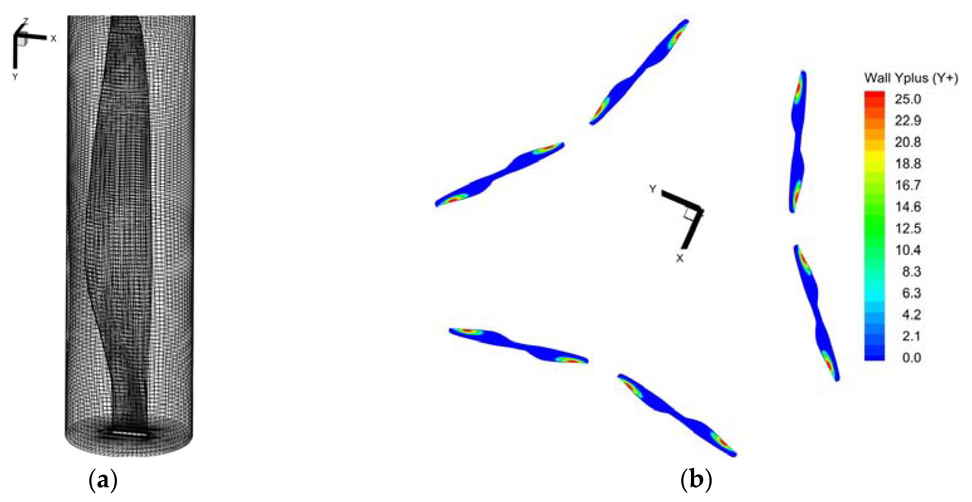
2. Computational Fluid Dynamics Model and Experimental Verification for Downwash Airflow

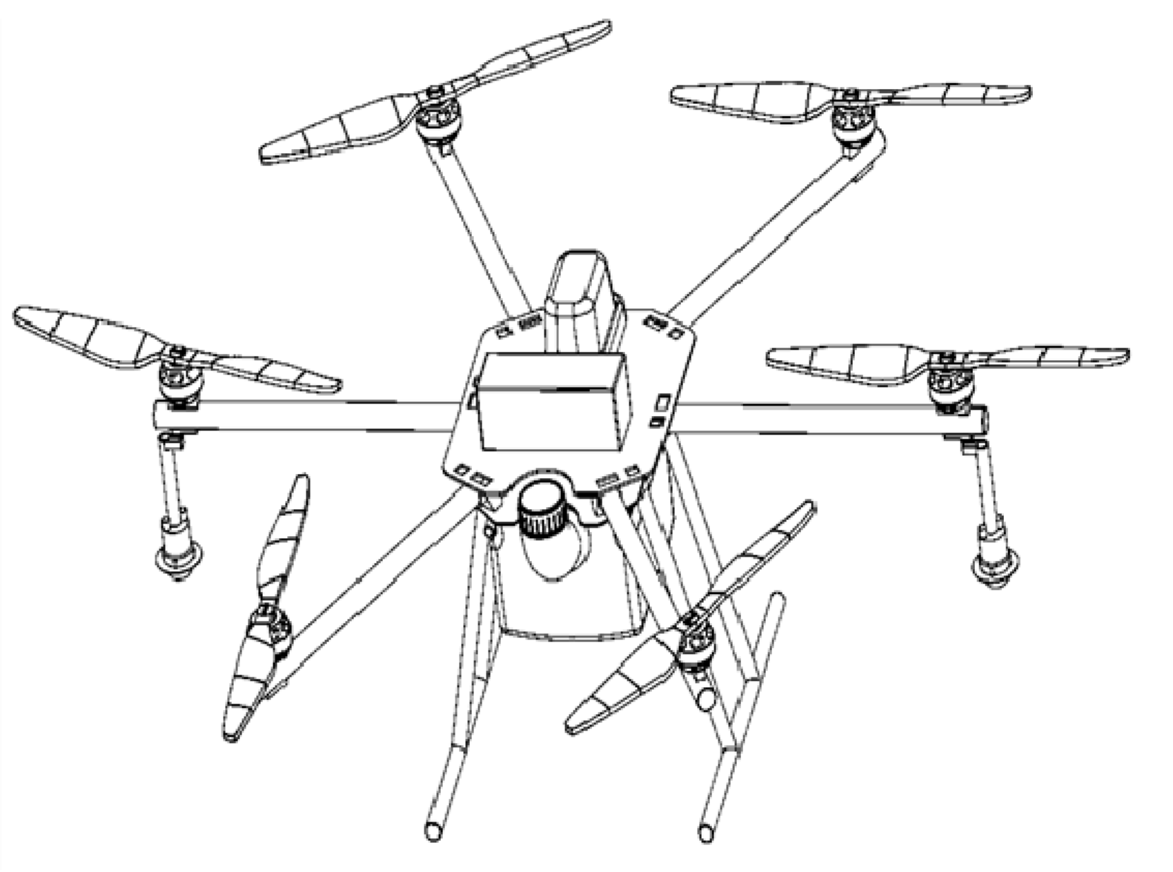
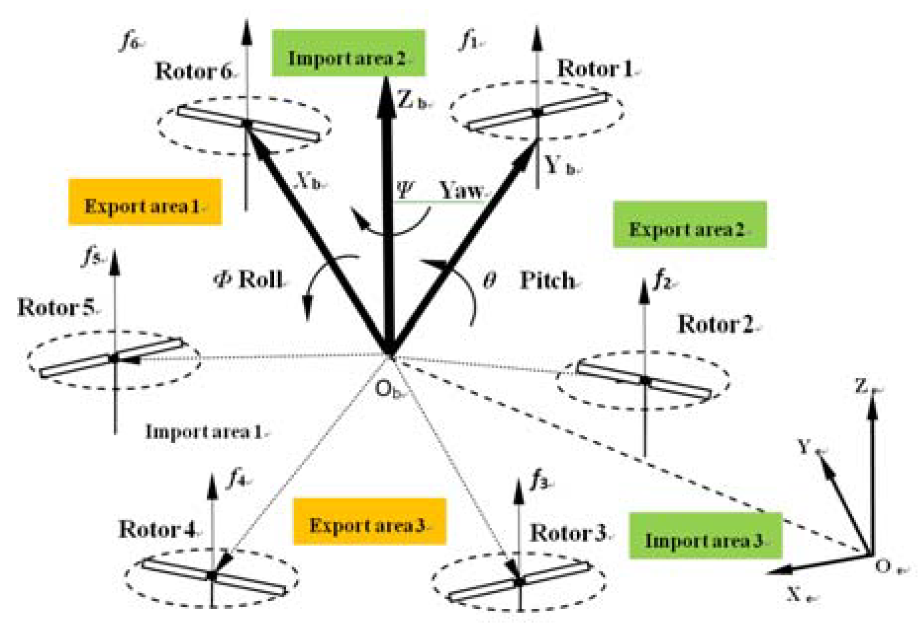
2.1. Working Principle of the SLK-5 Six-Rotor UAV

The SLK-5 plant protection UAV in this paper, as shown in Figure 1, is provided by the Xian Wideworldz Aviation Science and Technology Limited Corp, which is located in Xi’an City, Shanxi Province, China.

The movement law of the SLK-5 six-rotor plant protection UAV is shown in Figure 2. Six rotors are uniformly distributed along the circumferential direction, and the lengths of the rotor support arms are equal, and the included angle between any two arms is 60°, and rotation directions of the adjacent rotors are contrary, as shown in Figure 2.

In Figure 2, O_eX_eY_eZ_e is the absolute ground coordinate system, and O_bX_bY_bZ_b is the relative coordinate system of the six-rotor UAV system itself. Lifting forces (f_i, i = 1, 2, 3, 4, 5, 6) generated by each motor are proportional to the square of the rotational speed of the rotor, and the flight attitude (composed of the Ψ, θ, and Φ corners) of the UAV can be accomplished to match load capacity by adjusting the speed of the six motors. While increasing the rotational speed of each rotor, the total lifting force is sufficient to overcome the gravity of the UAV itself, and the UAV will rise. On the contrary, while reducing the rotational speed of each rotor, so that the total lifting force is less than gravity, the UAV descends. Similarly, when the lift generated by the rotors and the UAV gravity are equal, the UAV will be in a hover state.

2.2. Wind Speed Test and Verification of Downwash Airflow Model

For the independent rotating hovering flow field, the coordinate system can be attached to the UAV. Compared to the fixed coordinate system, the Reynolds Averaged Navier Stokes (RANS) equation in the rotating coordinate system is attached with a source term, $\mathit{Q}$, due to rotation. The specific form of the equation can be expressed as [25]

$$\frac{\partial }{\partial t}{\displaystyle \underset{\partial Vol}{\iiint }WdVol}+{\displaystyle ∯\left[\mathit{F}(\mathit{W})-\mathit{G}(\mathit{W})\right]}d\overrightarrow{S}={\displaystyle \underset{\partial Vol}{\iiint }\mathit{Q}dVol},$$

(1)

$$\mathit{W}=\left[\begin{array}{l}\rho \\ \rho u\\ \rho \nu \\ \rho w\\ \rho E\end{array}\right]\mathit{F}(\mathit{W})=\left[\begin{array}{l}\rho (q_n-q_b)\\ \rho u(q_n-q_b)+p{\stackrel{⌢}{n}}_x\\ \rho \nu (q_n-q_b)+p{\stackrel{⌢}{n}}_y\\ \rho w(q_n-q_b)+p{\stackrel{⌢}{n}}_z\\ \rho H(q_n-q_b)+p{q}_b\end{array}\right]\mathit{G}(\mathit{W})=\left[\begin{array}{c}\hfill 0\hfill \\ {\tau }_{xx}{n}_x+{\tau }_{yx}{n}_y+{\tau }_{zx}{n}_z\hfill \\ {\tau }_{xy}{n}_x+{\tau }_{yy}{n}_y+{\tau }_{zy}{n}_z\hfill \\ {\tau }_{xz}{n}_x+{\tau }_{yz}{n}_y+{\tau }_{zz}{n}_z\hfill \\ {\Phi }_x{n}_x+{\Phi }_y{n}_y+{\Phi }_z{n}_z\hfill \end{array}\right]\mathit{Q}=\left[\begin{array}{c}0\\ \rho w\Omega \\ 0\\ -\rho u\Omega \\ 0\end{array}\right],$$

(2)

where $\mathit{W}$ is the conserved variable vector, $\mathit{F}(\mathit{W})$ and $\mathit{G}(\mathit{W})$ are non-viscous flux and viscous flux respectively, $\mathit{Q}$ is the source term caused by rotor rotation; $\rho$ and $p$ are the density and pressure of the fluid; $u$, $\nu$, $\omega$ are fluid velocity components; E is the internal energy of a fluid unit; $n=\left[{\stackrel{⌢}{n}}_x,{\stackrel{⌢}{n}}_y,{\stackrel{⌢}{n}}_z\right]$ denotes the normal vector of the control surface, $Vol$ denotes the unit volume, and $\Omega$ denotes rotating speed of rotor; $q_n=u{\stackrel{⌢}{n}}_x+\nu {\stackrel{⌢}{n}}_y+\omega {\stackrel{⌢}{n}}_z$ and $q_b=u_b{\stackrel{⌢}{n}}_x+{\nu }_b{\stackrel{⌢}{n}}_y+{\omega }_b{\stackrel{⌢}{n}}_z$ denote fluid velocity and grid speed along the normal direction of mesh surface respectively; ${\tau }_{xx/yy/zz}$, ${\tau }_{xy/xz/yz}$ and ${\Phi }_{x/y/z}$ are the related viscous quantities; $\mu$, $k$, T denote viscosity coefficient, thermal conductivity, and absolute temperature, respectively.

In this paper, the SLK-5 six-rotor plant protection UAV provided by Xi’an Wade Ward Aviation Science and Technology Limited Corp which is located in Xi’an City, Shanxi Province, China, is taken as the research object. In reference [17], the flow field calculation and detailed analysis of the six-rotor plant protection UAV under no load hover condition were performed. Based on this work, the numerical calculation and test verification of the downwash airflow under the condition of 3 kg load are carried out.

The unsteady calculation of the downwash airflow field under the condition of 3 kg load is carried out. The time step of the initial segment is 1 × 10⁻⁵ s. After the residual is stable, the time step is 5 × 10⁻⁵ s. When the calculation time reaches about 2.28 s, the hovering downwash airflow flows to the ground, and tends to be stable.

The thickness of the first layer-covering rotor has a great influence on the airflow field and aerodynamic characteristics, and the index for evaluating the grid model is Y+ [26] of the rotor wall after numerical calculation, as in Equation (3):

$$Y+=\frac{\Delta y\rho }{\mu }\sqrt{\frac{{\tau }_{\omega }}{\rho }},$$

(3)

where Δy is the distance from the first layer of mesh to the surface of the object; ρ is the fluid density; μ is the viscosity of the fluid; and τ_ω is the surface shear stress of the model. Equation (3) shows that the Y+ value is proportional to the first layer thickness of the grid.

In most areas, the Y+ value is below 10. The Y+ value is greatest in the separation zone of airflow and rotor, but Y+ is basically controlled below 25. Generally speaking, the meshing quality of the rotor basically meets the calculation requirements of the downwash airflow, as shown in Figure 3.

The wind speed test points are arranged under the rotor, the height of the aircraft’s rotor from the ground is 3.25 m, and the height from the ground is 2.55 m and 1.55 m, respectively. There are 12 test points in total, and the plant protection UAV has a load of 3 kg when hovering. The “Kestrel 4500” digital anemometer is used to measure the velocity of the 12 measuring points in Z direction. The wind speed test site is based on reference [17]. The test is conducted in breezy weather with a natural wind speed of 0.2–0.3 m/s and a temperature of 32 °C. The 12 average pulsation values of the measured points in the Z direction after stabilization are 9.1, 9.3, 9.0, 9.1, 9.2, 9.1, 6.1, 6.3, 6.4, 5.9, 6.0, and 6.2 m/s respectively. The average values of wind speed pulsation at the observation point after numerical calculation are 9.50, 9.6, 9.56, 9.7, 9.6, 9.75; 6.52, 6.7, 6.63, 6.35, 6.5, and 6.39 m/s respectively. The comparison results are shown in

Table 1. Experimental and simulation values of the z-direction velocity for the marked points: (a) Marked points below the first three rotors; (b) Marked points below the last three rotors.

Height (m)	Rotor 1			Rotor 2			Rotor 3
	CFD (m/s)	Test (m/s)	Error(%)	CFD (m/s)	Test (m/s)	Error(%)	CFD (m/s)	Test (m/s)	Error(%)
2.55	9.50	9.10	4.4	9.6	9.30	3.8	9.56	9.00	6.2
1.55	6.52	6.10	6.9	6.7	6.30	7.1	6.63	6.40	3.6
Height(m)	Rotor 4			Rotor 5			Rotor 6
	CFD (m/s)	Test (m/s)	Error(%)	CFD (m/s)	Test (m/s)	Error(%)	CFD (m/s)	Test (m/s)	Error(%)
2.55	9.70	9.10	6.6	9.70	9.10	6.6	9.70	9.10	6.6
1.55	6.35	5.90	7.6	6.35	5.90	7.6	6.35	5.90	7.6

.

Figure 4b,c show the velocity distribution of the yoz and xoz sections after the downwash airflow calculation is stabilized, and Figure 4d shows a detailed streamlined diagram of the xoy section at z = 1.226 m under pressure background. It can be seen from Table 1 that the wind speed test error is controlled within 9%, indicating that the numerical calculation basically meets the accuracy requirements of engineering calculation. It can be seen from Figure 4 and Table 1 that the single point wind speed measurement has limited research effect on the wind field, and the detailed description of the wind field is weak. Numerical simulation can be used as an effective means to study wind field evolution and flow law, and is an effective supplement to single point wind speed test.

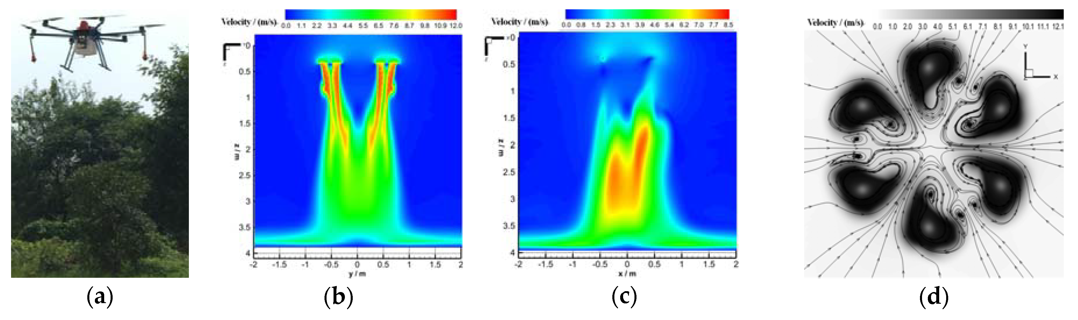
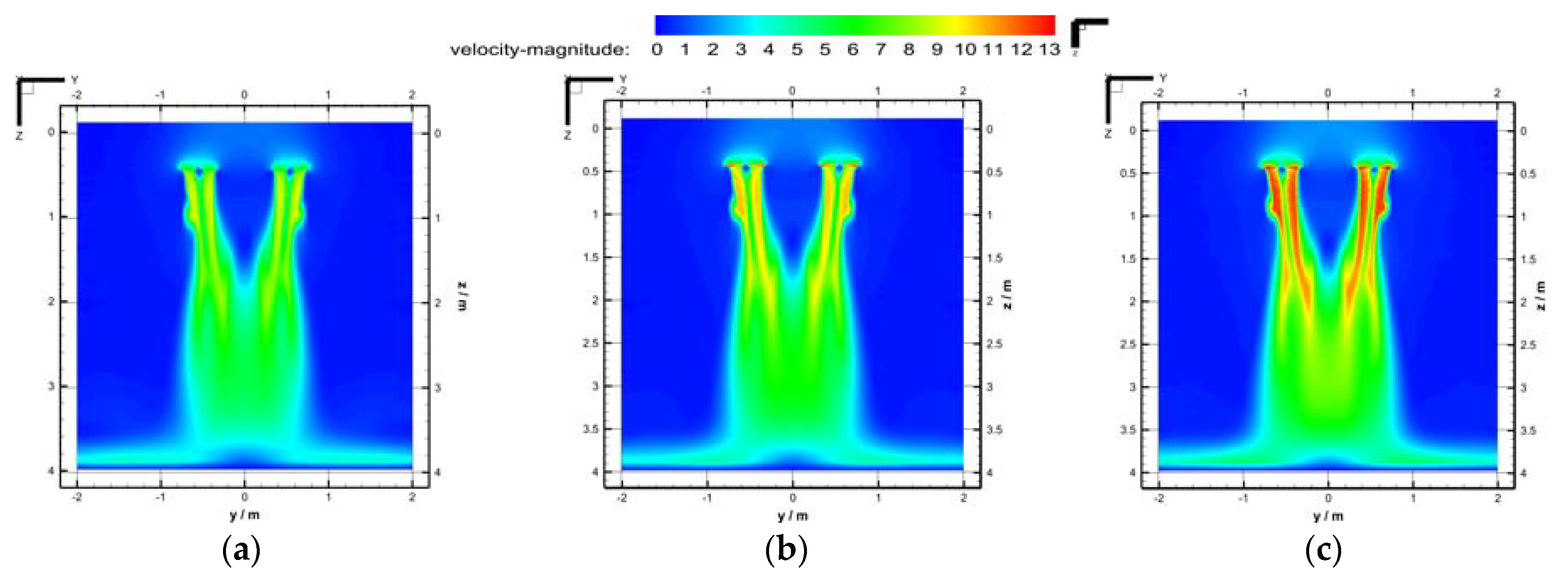
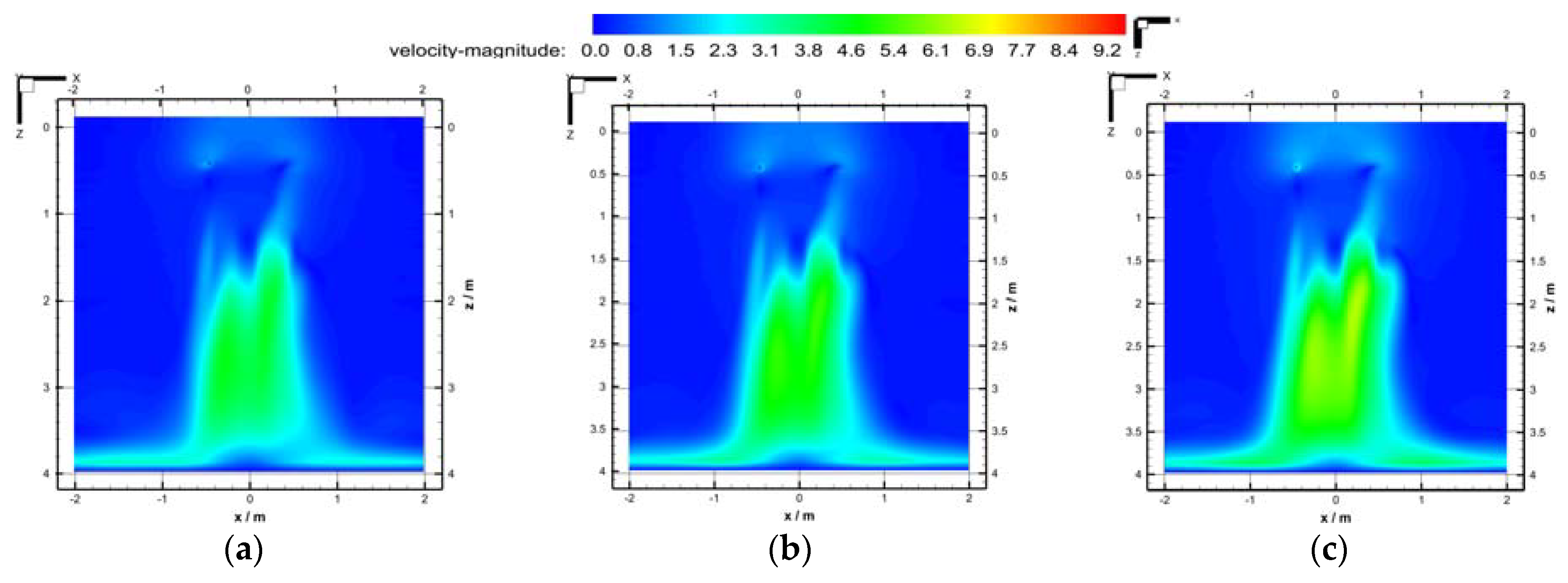
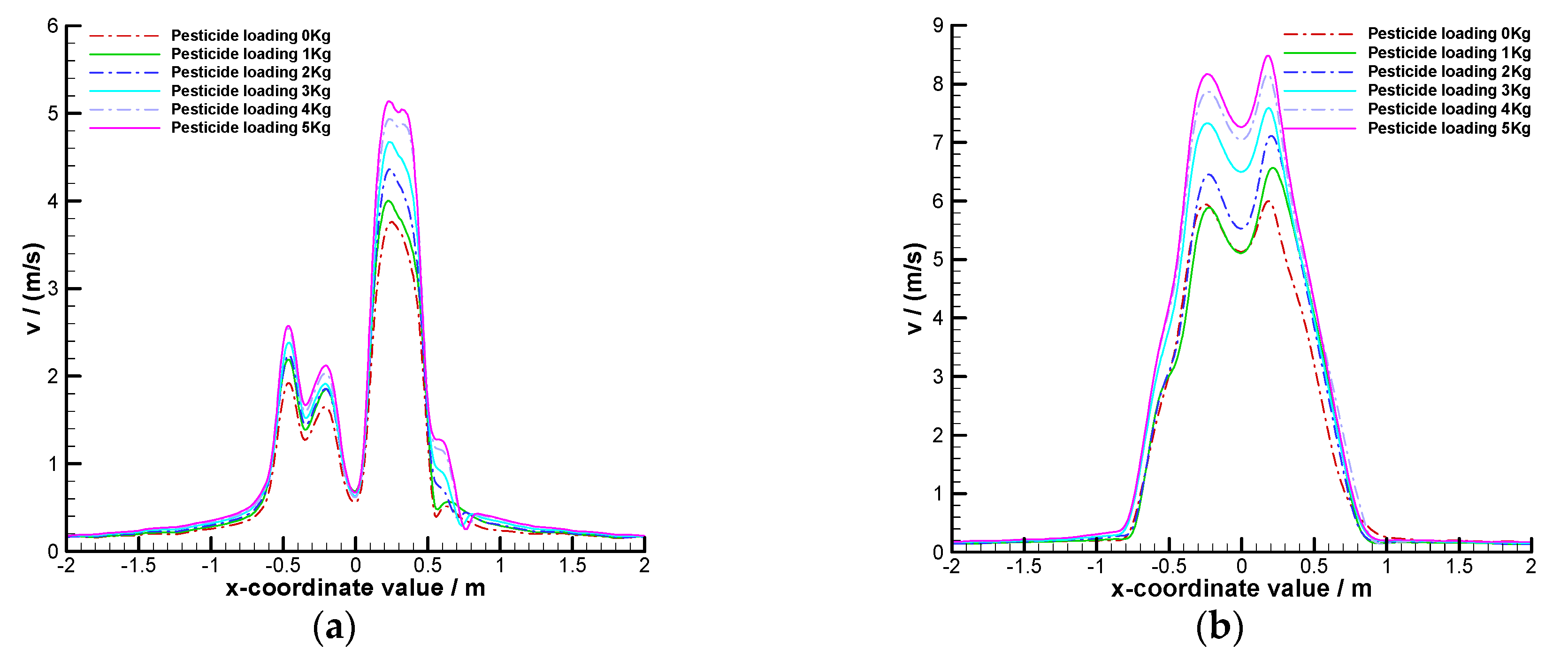
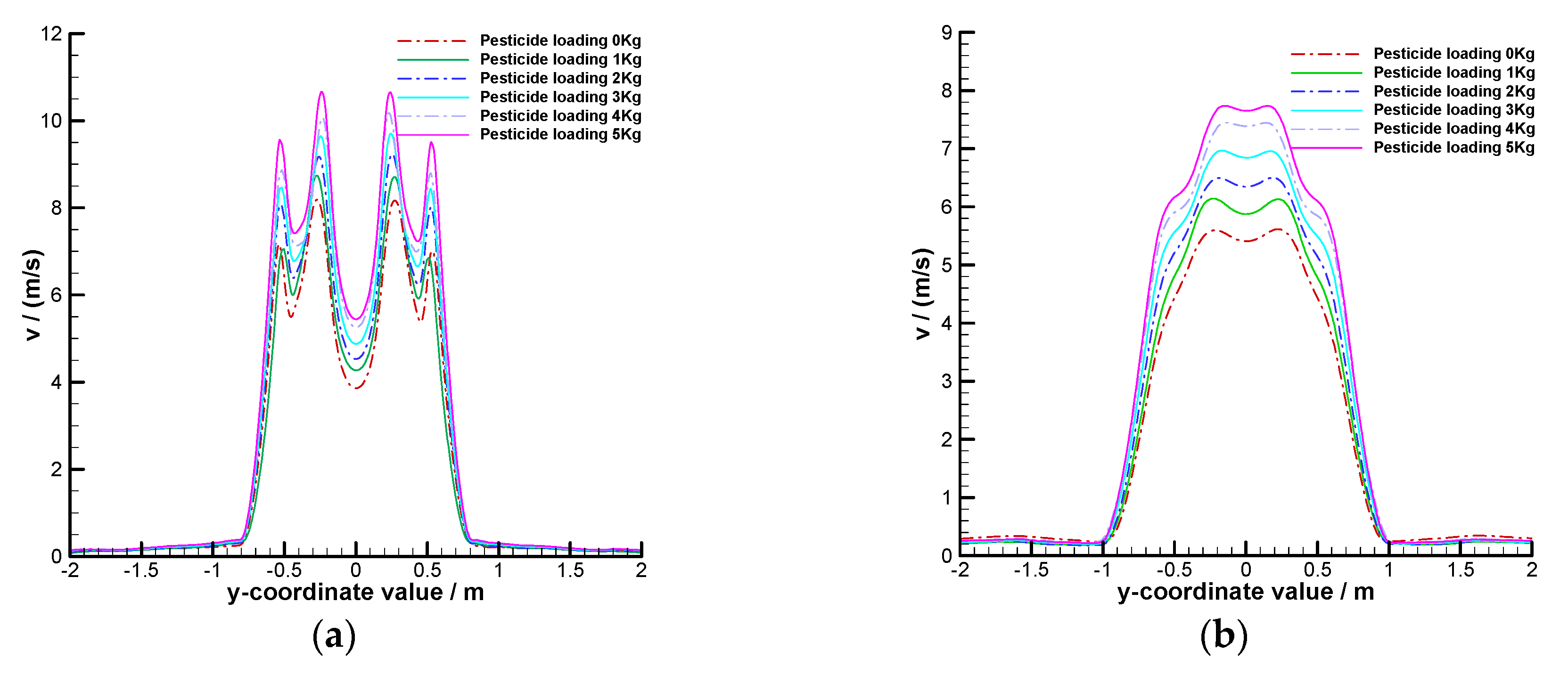
2.3. Effect of Load on Downwash Airflow Distribution in Hover

The distributions of the downwash flow under no-load, load of 1, 2, 3, 4, and 5 kg, are studied. Due to space limitations, Figure 5 and Figure 6 show the results of three working conditions.

Figure 5 shows that the larger the load, the greater the wind speed in the downwash zone when the plant protection UAV is hovering. Among the five working conditions, after the development of the downwash airflow is stable, the maximum wind speeds in the downwash area are 9.14, 9.92, 10.51, 11.1, 11.8, and 12.35 m/s, respectively. The yoz cross-section velocity cloud shows that the downwash airflow region exhibits the “trumpet” shape that “first contracts and then expands”. Among them, under the conditions of no load and low load, the phenomenon of “contraction, post expansion, and re-contraction” appears in the downwash area. The following analysis can be carried out. In the core area of the downwash airflow, the airflow speed is relatively large, so that the pressure in the region is significantly smaller than the peripheral air pressure, resulting in an external force of the atmosphere compressing the center of the downwash zone. The wind speed is attenuated as the downwash airflow develops toward the ground, the pressure resistance is weakened, and the “first contraction” phenomenon occurs in the downwash airflow; with the further development of the downwash airflow, the two downwash streams of the yoz section contract inwardly and merge together, so that the pressure in the downwash zone is greater than the outside air pressure, the downwash zone expands, and there is a phenomenon of “post expansion” of the downwash airflow.

As can be seen from Figure 2 and Figure 6, due to the existence of inter-wing interference (caused by the opposite turns of adjacent rotors), the asymmetry of the downwash airflow velocity in this section is obvious. Before the downwash airflow meets, the inter-wing interference phenomenon has a great influence on the wind speed of the xoz section. The “import zone” has an independent wind speed peak zone, and the “export zone” has a lower wind speed value.

Figure 7 and Figure 8 show the wind speed value curves at different heights (z direction) on the yoz section and the xoz section after the downwash airflow is stabilized. There are four “peaks” with symmetric distributions in the yoz cross-section, and the two “peaks” on the inner side are obviously higher. The three “valleys” are symmetrically distributed at the center of the section. As the downwash airflow continues to flow downward and meet, the two “peaks” on the outside weaken and disappear; the distance between the two inner “peaks” gradually shortens, and the wind speed values of “peaks” and “valleys” tend to coincide. As can be seen from Figure 8, the wind speed distribution in the xoz section is completely asymmetrical, and two obvious “peaks” appear. The “wing interference” phenomenon makes the difference between the two “peaks” obvious. As the vertical distances from the rotor get further and further away, the sides of the downwash airflow gradually merge, and the “peak” difference becomes smaller and smaller.

3. Two-Phase Computational Fluid Dynamics Model and Experimental Verification

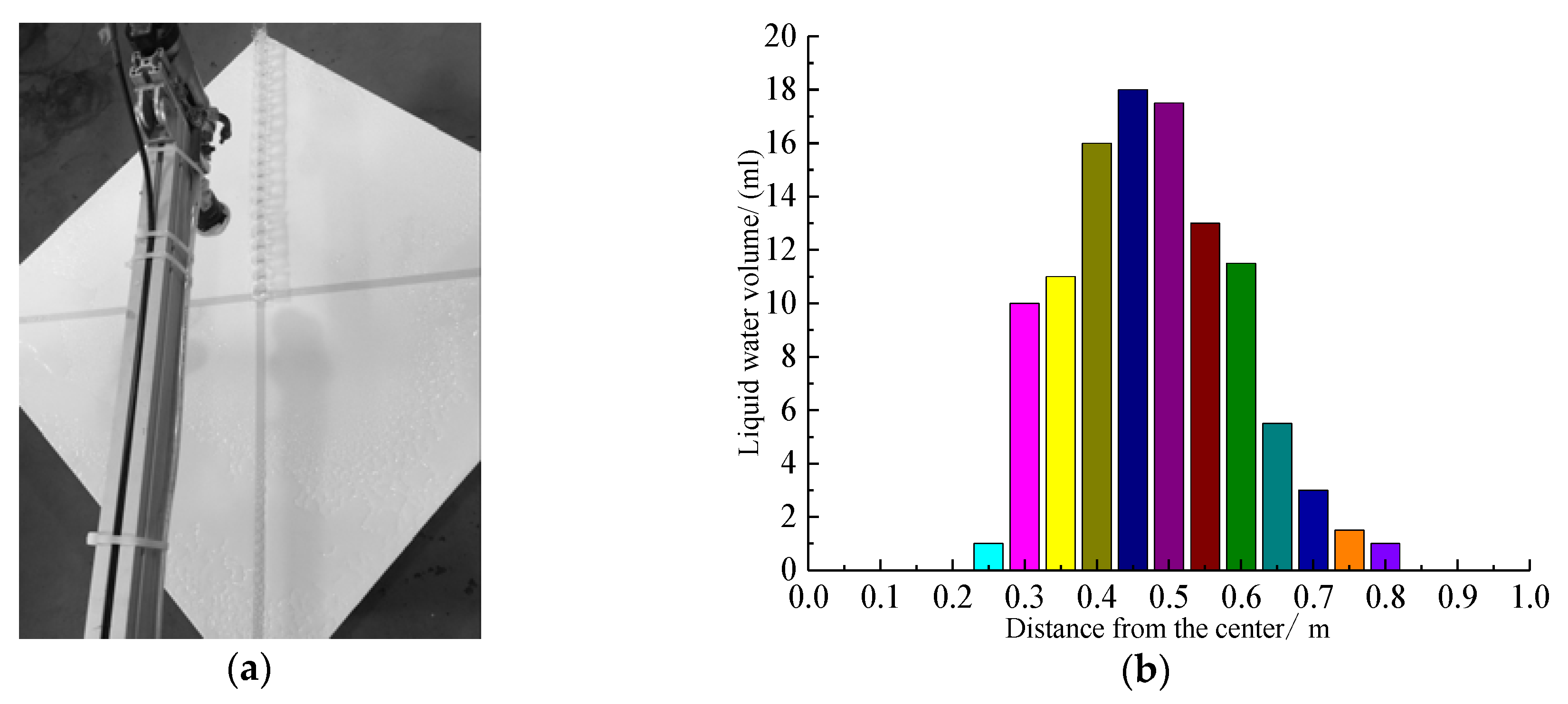
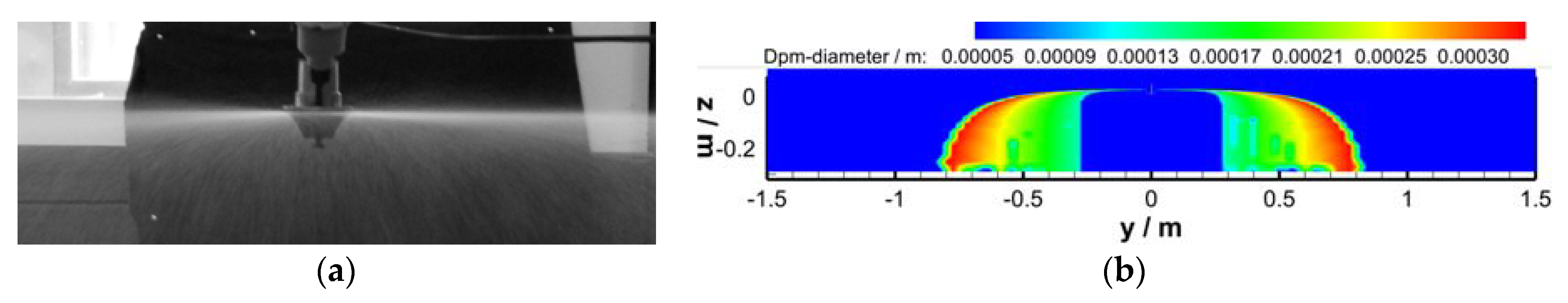
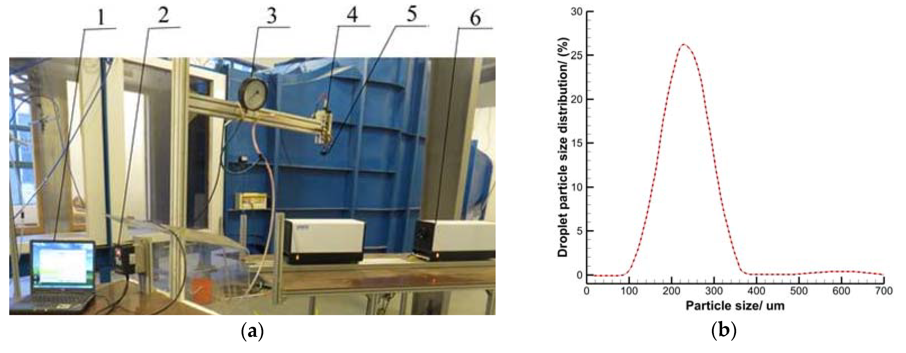
3.1. Droplet Particle Size and Spray Width Test

The outdoor gust phenomenon is more serious, as the hovering downwash airflow field is disturbed by the strong and weak cross wind, which brings strong interference to the measurement of droplet deposition. In addition, the main structure of the laboratory is steel, so the UAV cannot stably accept the BDS/GPS signal indoors, which poses a great safety hazard to the flight. In view of this, the experiment test is conducted in an indoor environment. The six-rotor plant protection UAV is equipped with a centrifugal atomization nozzle. The particle size test and the spray width test analysis of the centrifugal atomization nozzle are carried out to analyze the movement law of droplet group. Based on the experiment, a two-phase flow calculation model with droplet movement is established and verified. The particle size distribution of the centrifugal atomizing nozzle is tested by the test system, as shown in Figure 9a.

The rated voltage of the diaphragm pump of the liquid supply system is 12 V, the pump flow rate is 700 mL/min, and the particle size measurement system consists of a DP-02 laser particle size analyzer and a laser particle size analysis system. The working parameters and operation of this system are as follows: adjust the frequency of the inverter so that the rotor speed is 3600 r/min, adjust the return valve opening to achieve a flow rate of 700 mL/min, the temperature of the test chamber is (30 ± 2) °C, the relative humidity is 35 ± 10%, outlet of the nozzle is 0.3 m away from the ground, there is no wind in the room, open the laser particle size analyzer, and preheat it for 15 minutes. Open the droplet size test software, adjust the system automatically, so that the background light is the highest in the 0 ring light column, the height of the first ring is less than 1/4 of the 0 ring, and the height of all the 12 rings light column decrease in turn. Filter out the background light and start spraying. After the measurement and statistics are completed, the spray is stopped, and the average differential distribution of the obtained droplets is measured, as shown in Figure 9b.

In this paper, a double-injection centrifugal atomizing nozzle is used. The water injection port is 180° apart and perpendicular to the bottom of the cup, which basically ensures the spray distribution uniformity of the nozzle in all directions. The test plan for spray width of this nozzle is shown in Figure 10a. In the four orthogonal directions (the length of each direction is 1 m), 21 identical small beakers are placed in sequence. After 10 minutes of spraying, the measuring cylinder is used to measure the amount of mist in the beaker, and the working conditions are the same as for the droplet size measurement.

The origin of the coordinate is directly below the rotor cup. The average values of the droplet deposition in the four directions after the test are shown in Figure 10b (the default is 0 when the liquid water deposition is less than 0.5 mL), and it can be seen from Figure 10b that the amount of droplet deposition increases first, and then decreases with the distance from the spray center getting further and further. When the accumulated amount of deposition is equal to 95% of the sum of the deposited mist, the corresponding droplet deposition position is taken as the effective boundary of the droplet drop point, which is shown as 0.75 m.

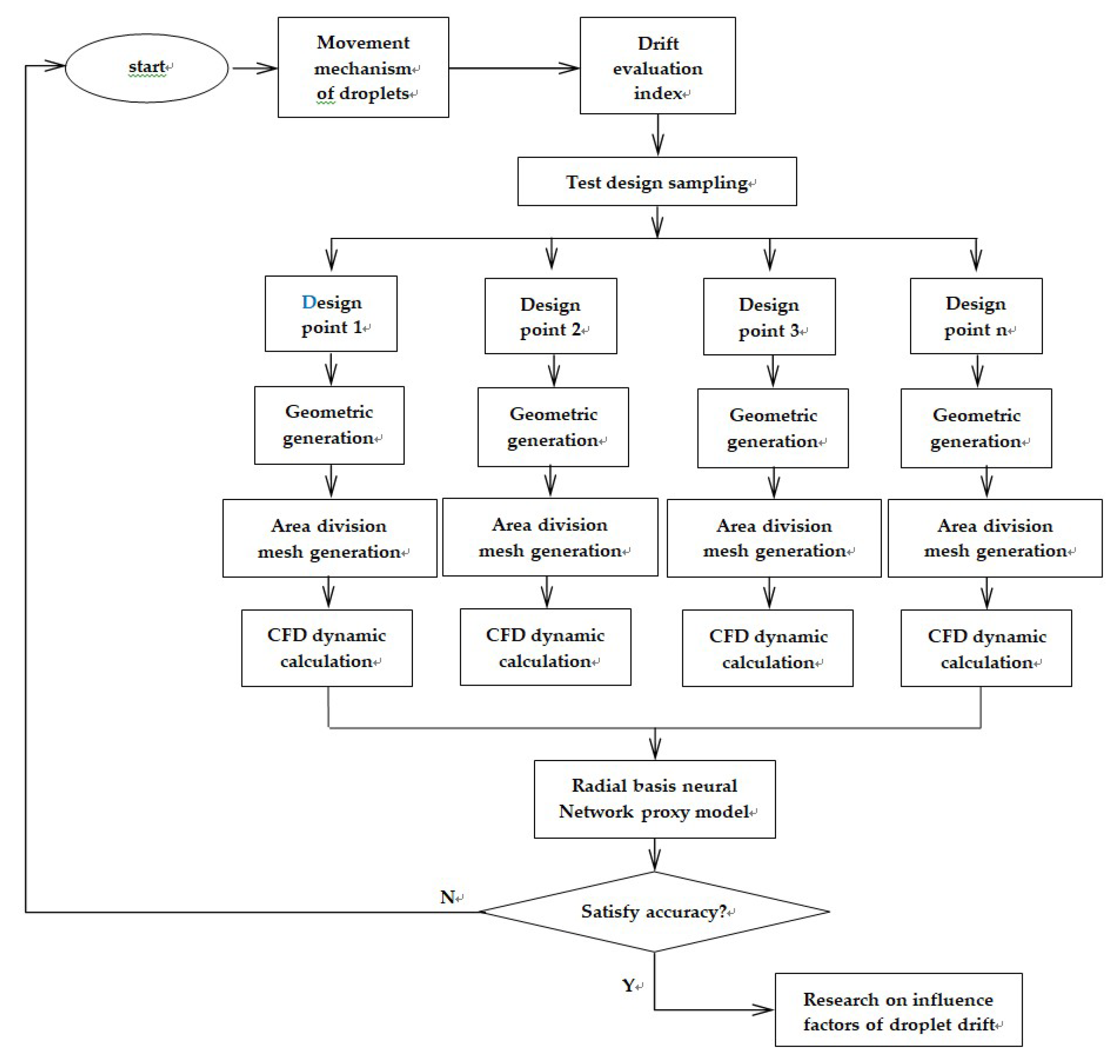
3.2. Two-Phase Numerical Calculation of Discrete Droplet Motion Law

The atomization process of the liquid in the rotor cup is not considered, and the inverse physical process of discrete phase liquid droplets becoming liquid continuous phase is not discussed. Discrete phase model is used as a research object to study the motion law of droplets under the influence of wind field.

Basic assumptions in this paper: (1) the air is ideal gas, obeys the ideal gas state equation; (2) the droplet is spherical, the speed of the downwash airflow is small, and the droplet breakage is not considered; (3) the effect of droplet evaporation is not considered.

In addition to gravity, the droplet is subject to various forces in the wind field, including viscous force, inertial force, and flow field pressure gradient force. The droplet volume is small, so the rotation motion is neglected, and the discrete phase motion equation is solved according to the Euler–Lagrange method proposed by Crowe and Smoot [27]:

$$\frac{\mathrm{d}{\mathit{v}}_{par}}{\mathrm{d}t}=\mathit{g}\frac{{\rho }_{par}-\rho }{{\rho }_{par}}+F_D(\mathit{v}-{\mathit{v}}_{par})+{\mathit{F}}_M+{\mathit{F}}_p,$$

(4)

$$F_D=\frac{3\mu }{{\rho }_{par}{d}_{par}^2}\frac{C_D\mathit{R}\mathit{e}}{4},$$

(5)

$$C_D=K_1+\frac{K_2}{\mathit{R}\mathit{e}}+\frac{K_3}{R{\mathit{e}}^2},$$

(6)

$$Re=\frac{{\rho }_f{d}_{par}\left|{\mathit{v}}_{par}-\mathit{v}\right|}{\mu },$$

(7)

$${\mathit{F}}_M=\frac{1}{2}\frac{\rho }{{\rho }_{par}}\frac{d\left(\mathit{v}-{\mathit{v}}_{par}\right)}{dt},$$

(8)

$${\mathit{F}}_p=\frac{\rho }{{\rho }_{par}}\left({\displaystyle \sum _i{\mathit{v}}_{par,i}\frac{\partial \mathit{v}}{\partial x_i}{\mathit{e}}_i}\right),$$

(9)

where v_par is the droplet velocity vector, the first term on the right side of Equation (4) is the superposition of gravity and fluid buoyancy, the second term indicates the viscous force, the third F_M is the force generated by the interaction between the fluid and the droplet, and the fourth term, F_p, is the force generated by the pressure gradient, F_D is the viscous force coefficient, C_D is the drag coefficient, and $\mathit{R}\mathit{e}$ is the Reynolds number expression.

The momentum change of droplet is caused by the airflow field. While the airflow affects the droplet motion, the drop motion also affects the airflow field, and there are momentum exchanges between the droplet group and airflow field.

The Equation (1) has 5 partial equations: the first partial equation is the mass conservation equation, the second to the fourth are the momentum conservation equations, and the fifth is the energy conservation equation. Suppose there are N_p droplets in the airflow field control unit, and the momentum effects generated by all the droplets on the airflow field are added to the right side of the momentum conservation equation in the form of source terms, then

$$S_{Mi}=-\frac{1}{Vol}{\displaystyle \sum _{i=1}^{N_p}\left[F_{D,i}\left(\mathit{v}-{\mathit{v}}_{par,i}\right)+{\mathit{F}}_{M,i}+{\mathit{F}}_{p,i}\right]m_{par,i}},$$

(10)

where m_par,j is mass of the i-th droplet in the control unit, v_par,i indicates the velocity vector of the i-th droplet, F_D,i is the viscous force of the i-th droplet, F_M,i is the force generated by the interaction between the airflow and the i-th droplet, F_P,i indicates the force generated by the airflow pressure gradient on the i-th droplet.

There is heat exchange between droplet group and airflow field, causing changes in the temperature distribution of the droplets and airflow field. The heat exchanges between all the droplets and the airflow field inside the control body are added to the right side of the energy conservation equation in the form of a source term.

$$S_H=-\frac{1}{Vol}{\displaystyle \sum _{i=1}^{N_p}{m}_{par,i}}{k}_{par,i}{A}_{par,i}\left(T-T_{par,i}\right),$$

(11)

where A_par,i is surface area of the i-th droplet, T_par,i is airflow field temperature in the volume control unit, and k_par,i indicates the transmission coefficient between the i-th droplet and airflow field.

The finite volume method is used to discretize the governing equations. To ensure the stability and convergence of the calculation, the coupling format is used for iteration. The airflow field calculation contains high speed rotation of the rotor, and the SST k–ω turbulence model is used to calculate turbulent flow field [28]. The STT k–ω turbulence model was developed by Menter [28] on the basis of the standard k–ω turbulence model. The definition of turbulent viscosity is adjusted according to the turbulent shear stress, which makes the model more suitable for the rotor flow field. The conservation transport equation of ρk and ρω can be expressed as

$$\frac{\partial \rho k}{\partial t}+\frac{\partial \rho k{v}_j}{\partial x_j}-\frac{\partial }{\partial x_j}\left(\frac{{\Gamma }_k}{{\mathrm{Re}}_r}\frac{\partial k}{\partial x_j}\right)=\frac{{\mu }_t}{{\mathrm{Re}}_r}{S}^2-\rho {\beta }^{\ast }k\omega ,$$

(12)

$$\frac{\partial \rho \omega }{\partial t}+\frac{\partial \rho \omega v_j}{\partial x_j}-\frac{\partial }{\partial x_j}\left(\frac{{\Gamma }_{\omega }}{{\mathrm{Re}}_r}\frac{\partial \omega }{\partial x_j}\right)=\rho \alpha S^2-\rho \beta \omega \omega +2\left(1-F_1\right)\rho {\sigma }_{\omega ,2}\frac{1}{\omega }\frac{\partial k}{\partial x_j}\frac{\partial \omega }{\partial x_j},$$

(13)

where each parameter in the formulas can refer to reference [28], and the turbulence model is very complicated, which this paper does not explain in detail.

According to the spray width test scheme, a three-dimensional two-phase flow model with droplet discrete phase is established. Due to the large number of droplets, the calculation amount of the droplet trajectory is very large, and the calculation domain is limited to a certain height in order to reduce the amount of calculation. Combined with the spray width test, after the droplets drop 0.3 m under no wind condition, the droplets basically reach the maximum spray width, so the sedimentation height of the droplets is set to 0.3 m. The atomization disk has a diameter of 58 mm and a height of 10 mm. After the model is established, the hexahedral mesh reaches 1.737 million.

The rotation speed and flow rate of the nozzle are consistent with the Section 3.1, which are 3600 r/s and 700 mL/min, respectively. The droplets are evenly distributed at the nozzle outlet according to the differential distribution of the droplets in the test (to reduce the amount of calculation, the particle size range is set to 100 to 320 μm). The tangential velocity of the droplets leaving the atomizing disk is 10.9 m/s. After 1.56 s of unsteady numeral calculation, the calculated value of the spray width is about 0.8 m (shown in Figure 11b), which is in good agreement with the test value in Section 3.1, as shown in Figure 10b.

Decomposing Equation (4) in the Section 3.2 into the x-axis direction, it can be concluded that the horizontal velocity is mainly affected by the viscous force of the airflow, the interaction force between the airflow and the droplets, and the pressure gradient force. The latter two factors have the same effect on each droplet, and viscous force is the most important factor affecting the difference of droplet trajectory. Combining Equations (4)–(7), it can be concluded that the larger the droplet size, the smaller the horizontal reverse acceleration, the slower the horizontal velocity attenuation, and the larger the spray amplitude.

4. Droplet Movement Law of the Six-Rotor Plant Protection UAV Spraying

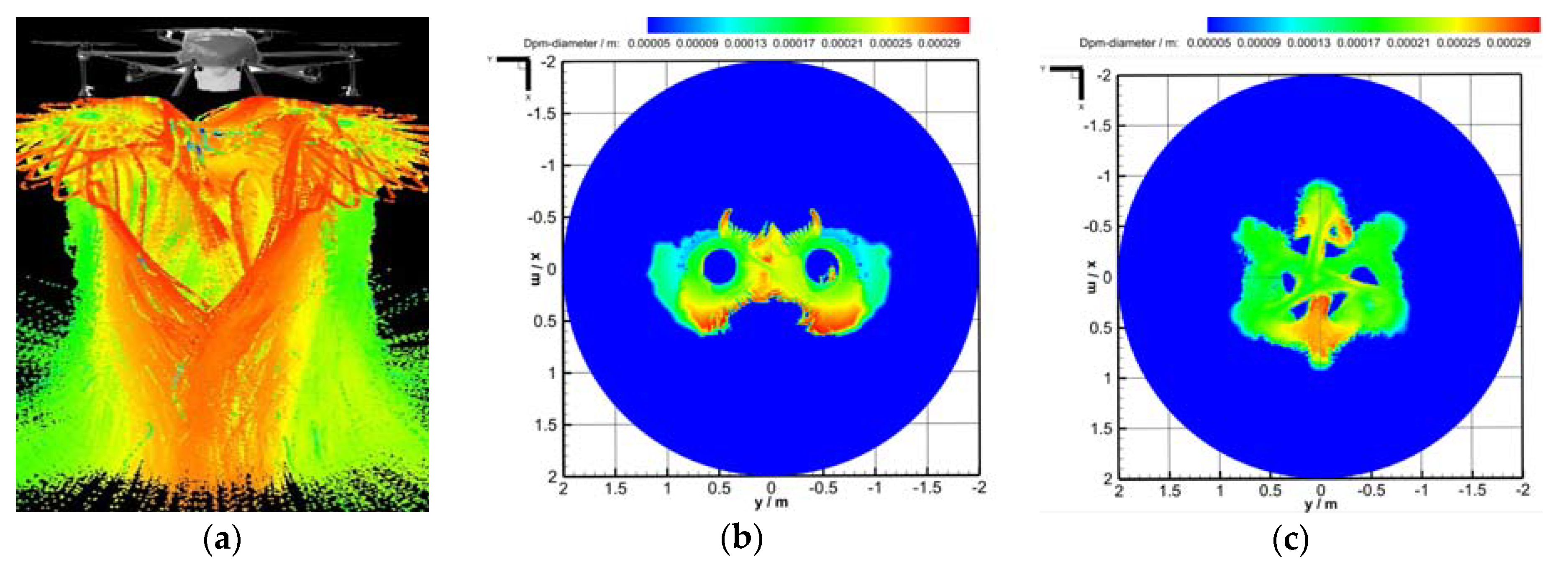
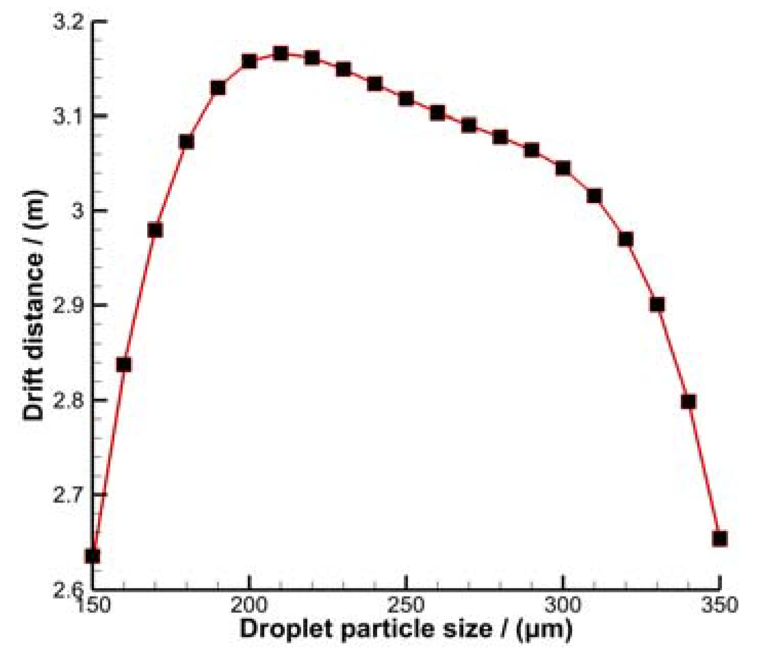
4.1. Influence of Downwash Airflow on Droplet Movement in Hover

On the basis of Section 2.2, a pair of nozzles are added at 235 mm directly below the corresponding rotors, to discuss the effect of the hovering downwash airflow on the droplet movement law (droplet size is the same as Figure 9b). The process is as follows: firstly, the unsteady calculation for the hovering downwash airflow of 3 kg load is carried out (the two nozzles are symmetrically distributed in the y-axis direction, and the rotation direction is consistent with the upper rotor). Secondly, after the downwash airflow develops to the ground and tends to stabilize, the two-phase flow model with droplet is activated, then the droplets are released, and the unsteady calculation is performed. Under the action of the downwash airflow, the motion and deposition laws tend to stabilize, and the calculation stops, then the results are extracted. Figure 12a shows the particle size distribution of droplets from a three-dimensional perspective. Due to the high-speed rotation of the rotor and nozzle, the droplet is affected by the downwash airflow and the circumferential induced force caused by the rotation of nozzle.

Under the disturbance of the downwash airflow under the rotor, the trajectory of the droplet does not show parabolic trajectory, but has a tendency of reverse motion after the lateral displacement reaches maximum. Finally, the lateral displacement of the droplet increases, again, under the influence of ground effect.

Figure 12b,c show the particle size distribution of the xoy cross-section at two heights of z = 1, 3 m after the two-phase flow is calculated. It can be seen from the combination of Figure 12b,c that the xoy cross-section of z = 1 m is the vicinity of the inflection point where the droplet undergoes a reverse movement after the lateral displacement reaches maximum. The droplets are gradually dispersed during the spiral descending motion. At z = 1 m, the droplets are not completely scattered, and the distribution is concentrated. With further spiraling down, the droplets gradually spread out at a height of z = 3 m, and the distribution is more uniform. Under the influence of the downwash airflow, the droplets gradually disperse during the spiraling process. From this level, as long as the flight altitude is appropriate, the multirotor UAV downwash airflow has positive significance for improving the droplet distribution in the downwash area.

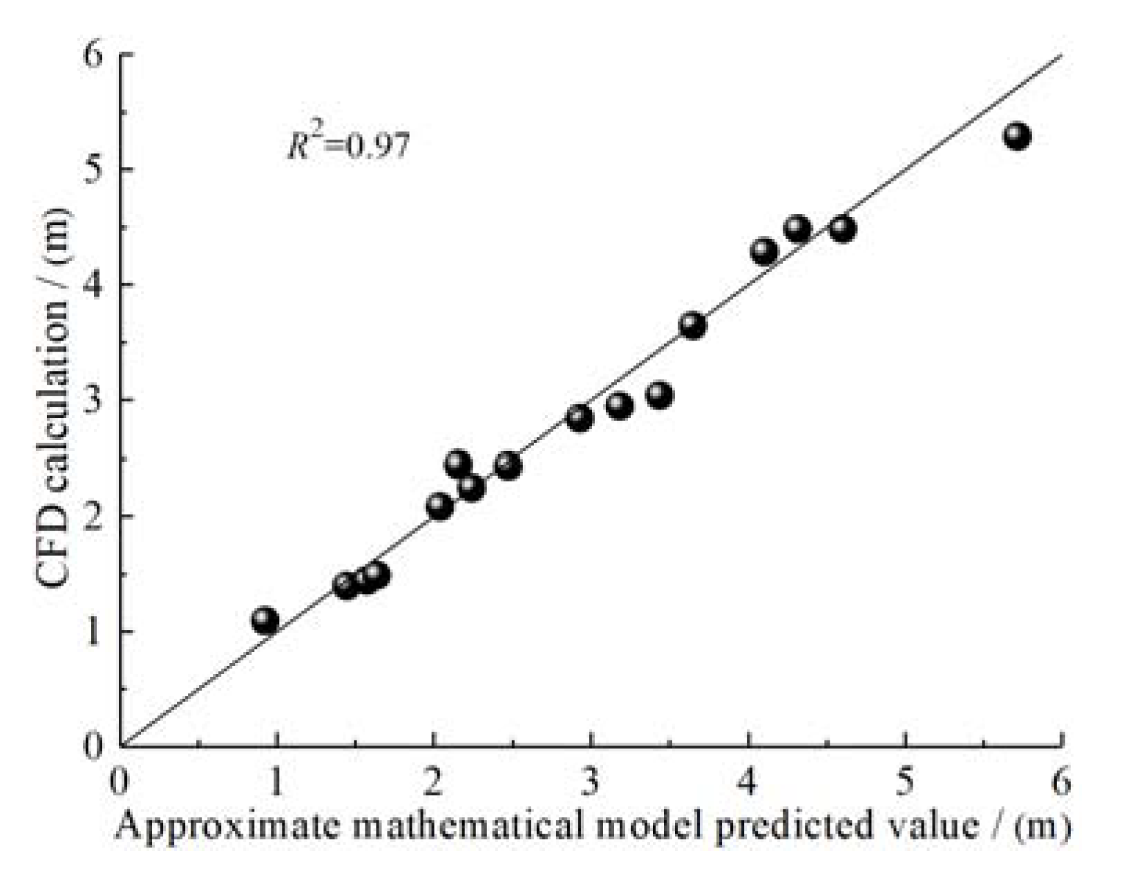
4.2. Droplet Drift Model

Under the influence of the coupled wind field, the drifting movement process of the droplet involves the interaction of the droplet and the airflow field, the exchange of momentum and energy between continuous phase and the discrete phase, and the turbulent pulsation of the flow field. What is even worse is that these factors are also coupled to each other. These factors make the multirotor plant protection UAV spraying drift model show strong nonlinearity. Before knowing the relationship between droplet drift and these factors, it is difficult for the authors to carry out specific research through a simple exhaustive method. Just increasing the number of samples in a large amount does not help us to completely understand the relationship between the drift and the relationship between these factors. What makes the situation worse is that every sample calculation based on CFD takes a lot of time. Therefore, it is an important issue for scholars to study an effective method to evaluate the nonlinear relationship between coupling wind field and drift characteristics.

Since the 1980s, a variety of approximate models have been developed which combine traditional experimental design with numerical techniques. This mainly includes response surface method, neural network method, kriging function method, and radial basis function method (RBF) [29,30]. However, Ruichen J. et al. [31] used 14 examples of different type problems to verify that the radial basis function model is relatively reliable when considering the accuracy and robustness of the model. Therefore, in this section, combined with computational fluid dynamics parameterization, optimization Latin hypercube experimental design, and RBF neural network structure, an implicit approximation mathematical model for multirotor plant protection UAV drift evaluation index is established, and research ideas and processes are shown in Figure 13.

The accuracy index of multirotor plant protection UAV drift model based on radial basis neural network is R², as follows:

$$R^2=\frac{S{S}_{Model}}{S{S}_{Total}},$$

(14)

where $S{S}_{Total}={{\displaystyle \sum _{}^m\left(\stackrel{}{y_i}-\stackrel{-}{y_i}\right)}}^2$ is the sum of squared total errors, $S{S}_{Mo\mathrm{del}}={{\displaystyle \sum _{}^k\left(\stackrel{\sim }{y_i}-\stackrel{-}{y_i}\right)}}^2$ is the squared error of the sample; m is the squared error of the sample, k is the number of samples (to ensure the reliability of the mathematical model, m is equal to k), $y_i$ is the actual value of the i-th sample, $\stackrel{\sim }{y_i}$ is the response value of the approximate mathematical model at the i-th sample point, and $\overline{y}$ is the mean value of the test sample response.

After multiple sampling, the sample space that satisfies the accuracy of the approximate model is shown in

Table 2. Sample space based on optimization Latin hypercube experimental design.

Sample Number	Vw/(m/s)	Dd/μm	LP Actual/m	LP Prediction/m
1	0.50	190.000	1.10	0.92
2	2.00	283.333	2.95	3.18
3	1.50	323.333	2.45	2.15
4	2.33	176.667	3.65	3.64
5	0.67	256.667	1.40	1.44
6	1.83	230.000	2.85	2.93
7	1.67	163.333	2.50	2.47
8	2.17	336.667	3.05	3.43
9	1.00	150.000	1.45	1.57
10	2.67	296.667	4.50	4.31
11	1.17	216.667	2.10	2.03
12	1.33	270.000	2.25	2.23
13	0.83	310.000	1.50	1.63
14	2.83	350.000	4.50	4.60
15	3.00	203.333	5.30	5.71
16	2.50	243.333	4.30	4.10

below, and the spatial distribution of the sample is shown in Figure 14 (V_w is windward velocity, D_d is droplet particle size, L_P is droplet drift distance). As can be seen from Figure 14, the distribution of sample points have good uniformity.

After a large number of samplings, calculations, and fittings by the parameterized platform, the approximation mathematical model has obtained satisfactory results. The six-rotor plant protection UAV drop drift model accuracy evaluation index R² is 0.97, as shown in Figure 15. It can be seen from Figure 15 that the predicted value of the mathematical model of the droplet drift agent agrees well with the sample value of the three-dimensional numerical calculation, which lays a good foundation for the study of the drift influence factor.

Since the approximation mathematical model constructed by the radial basis neural network is a non-explicit mathematical relationship, the approximate model is trained by MATLAB. Two independent variables “windward velocity a, droplet diameter b” and one dependent variable “drift distance f”, are defined, and the intelligent decision analysis of drift single influence factor is carried out. Relative to the reference model, the values of the windward airflow velocity and the droplet diameter are increased by 0.4 m/s and 20 μm respectively, and the drift distance corresponding values are given based on the drifting approximation mathematical model.

Figure 16 and Figure 17 respectively show the correspondence between the drift distance of the droplet and the windward speed in the 260 μm and other multiple particle size conditions. Figure 18 and Figure 19 show the corresponding relationship between the drift distance and particle size in the 2 m/s and other multiple wind speed conditions.

It can be seen from Figure 16 that, in the case where the droplet size is 260 μm, the drift distance of the droplet becomes longer and longer as the windward speed gradually increases. The drift distance of the droplet is controlled by the downwash airflow and the windward wind speed. When the windward speed is less than 1.75 m/s, the downwash airflow speed of the rotors can significantly affect the windward which, in turn, affects the lateral movement of the droplet, so, the lateral distance of the droplet increases slowly, and the increase of drift distance gradually decreases. When the windward speed is increased to 1.75 m/s or more, the influence of the windward airflow on the droplet movement is gradually higher than that of the rotor downwash airflow. Therefore, the lateral distance of the droplet increases faster, and the drift distance increases gradually.

In addition, as can be seen from Figure 17, as the particle size of the droplet increases, the correspondence between the droplet drift distance and the windward speed is different. When the windward speed is less than 0.75 m/s, as the droplet size increases gradually, the drift distance of the droplets becomes farther and farther, and this conclusion is similar to Section 3.2. We can also find that when the windward speed exceeds 1.75 m/s, the lateral distance of the droplet drift is much farther. On the other hand, decomposing Equation (4) in Section 3.2 into the z-axis direction, it can be concluded that, the smaller the droplet, the greater the resistance in the vertical direction by combining Equations (5)–(9). Hence, in general, when the windward speed is within 3 m/s, the larger the particle size, the farther the droplet drifts; but when the particle size reaches a certain level, the windward airflow becomes the dominant factor affecting the drift distance of the droplet, and the larger the particle size, the closer of the droplet drift, as shown in Figure 17.

Referring to Figure 4 and Figure 18, when the windward speed is 2 m/s and the particle size ranges from 150 to 350 μm, the drift distance of the droplet exceeds the downwash area. Figure 18 shows that, as the particle size increases, the drift distance of the droplet first increases and then decreases. This phenomenon can be explained from the following aspects. The droplet is subjected to forces in two directions after flying out of the centrifugal atomizing nozzle, namely, the vertical direction and the horizontal direction. The droplet drift distance depends on the combined effect of the two forces. Decomposing Equation (4) in Section 3.2 into the x-axis direction, it can be concluded that large droplets are less affected by horizontal forces (in the initial stage, the velocity of the droplet is greater than the windward speed, and the resistance of the large droplet is small. The driving force of the droplet is smaller after the horizontal velocity of the droplet is less than the wind speed), the lateral velocity of the initial segment decreases rapidly, and the lateral velocity of the latter segment is slower. On the other hand, decomposing Equation (2) in Section 3.2 into the z-axis direction, the droplet is simultaneously subjected to vertical resistance, and the large droplet is subjected to low resistance (gravity is downward, resistance is upward), and the falling speed is faster. In combination with the previous two points, the distance of the large droplet moving in the lateral direction is longer in the same time, and the time of the large droplet moving at the same longitudinal height is shorter; this is a contradiction.

Combined with the previous two points and Figure 19, we can see that the drift distance of the droplet during particle size increase has an inflection point that increases, first, and then decreases at different windward speed; and as the windward speed increases, the corresponding particle size of this inflection point becomes larger and larger.

The droplet size and windward speed are used as model input, and the droplet drift distance is output. The radial basis neural network method is used to write the program, and the input and output samples of the multidisciplinary parameterized platform are tested and trained. Finally, the six-rotor UAV spray drift prediction model is initially established, as shown in Figure 20.

5. Conclusions and Future Work

In the present paper, the influence of downwash airflow, windward airflow, and particle size on the motion distribution of droplet groups are studied for the SLK-5 six-rotor plant protection UAV. Based on the N-S equation and SSK k–ε turbulence model, the three-dimensional downwash airflow numerical model is established for the UAV under 3 kg load condition. Analysis shows that the relative error of the z-direction velocity between the experimental measurement and numerical simulation is less than 9%, so the reliability of the wind field numerical calculation is verified.

The two-phase flow model with droplet discrete phase is established for the nozzle, the relative error of the spray width between the experimental measurement and numerical simulation is less than 7%, and the feasibility and validity of the two-phase flow model for calculating the trajectory of the droplet are also verified, combined with the spray test. Then, the two-phase flow model is applied to the spray process of the SLK-5 six-rotor UAV in hover. The droplets on the inner side of the nozzle are interlaced, and the outer large droplets have a larger horizontal stroke and are distributed outside the downwash zone, and the droplets are mainly deposited in three “introduction areas” and three “export areas”, where “wing interference” is apparent.

Combining computational fluid dynamics parameterization, optimization of Latin hypercube experimental design, and a radial basis neural network, an implicit approximation mathematical model for drop drift of six-rotor plant protection UAV is established. Finally, based on this implicit model, the influences of the windward airflow speed and particle size on the droplet drifting law are discussed in detail under the disturbance of the downwash airflow.

References

1. Wang, C.; Song, J.; He, X.; Wang, Z.; Wang, S.; Meng, Y. Effect of flight parameters on distribution characteristics of pesticide spraying droplets deposition of plant-protection unmanned aerial vehicle. Trans. Chin. Soc. Agric. Eng. 2017, 33, 109–116. [Google Scholar]
2. Qin, W.; Xue, X.; Zhou, L.; Zhang, S.; Sun, Z.; Kong, W.; Wang, B. Effects of spraying parameters of unmanned aerial vehicle on droplets deposition distribution of maize canopies. Trans. Chin. Soc. Agric. Eng. 2014, 30, 50–56. [Google Scholar]
3. Bradley, K.F. Role of atmospheric stability in drift and deposition of aerially applied sprays-preliminary results. ASAE 2004, 58, 742–755. [Google Scholar]
4. Ivan, W.K.; Bradley, K.F.; Wesley, C.H. Aerial methods for increasing spray deposits on wheat heads. ASAE 2004, 58, 716–729. [Google Scholar]
5. Kirk, L.W.; Teske, M.E.; Thistle, H.W. What about upwind buffer zones for aerial applications? J. Agric. Saf. Health 2002, 8, 333–336. [Google Scholar] [CrossRef] [PubMed]
6. Xue, X.Y.; Lan, Y.B. Agricultural aviation application in USA. Trans. Chin. Soc. Agric. Mach. 2012, 44, 194–201. [Google Scholar]
7. Dumbauld, R.K.; Bjorklund, J.R.; Saterlie, S.F. Computer Models for Predicting Aircraft Spray Dispersion and Deposition above and within Forest Canopies: User’s Manual for the FSCBG Computer Program Report; No 80–11; US Forest Service: Davis, CA, USA, 1980. [Google Scholar]
8. Teske, M.E.; Thistle, H.W.; Schou, W.C.; Miller, P.C.H.; Strager, J.M.; Richardson, B.; Butler-Ellis, M.C.; Barry, J.M.; Twardus, D.B.; Thompson, D.G. A review of computer models for pesticide deposition prediction. Trans. ASABE 2011, 54, 789–801. [Google Scholar] [CrossRef]
9. Reed, W.H. An Analytical Study of the Effect of Airplane Wake on the Lateral Dispersion of Aerial Sprays; Langley Aeronautical Laboratory: Hampton, VA, USA, 1953. [Google Scholar]
10. Bilanin, A.J.; Teske, M.E.; Barry, J.W.; Ekblad, R.B. AGDISP: The aircraft spray dispersion model, code development and experimental validation. Trans. ASABE 1989, 32, 327–334. [Google Scholar] [CrossRef]
11. Teske, M.E.; Bird, S.L.; Esterly, D.M.; Curbishley, T.B.; Ray, S.L.; Perry, S.G. AgDrift®: A model for estimating near-field spray drift from aerial applications. Environ. Toxicol. Chem. 2002, 21, 659–671. [Google Scholar] [CrossRef] [PubMed]
12. Hewitt, A.J. Spray drift: Impact of requirements to protect the environment. Crop Prot. 2000, 19, 623–627. [Google Scholar] [CrossRef]
13. Hewitt, A.J.; Johnson, D.R.; Fish, J.D.; Hermansky, C.G.; Valcore, D.L. Development of the spray drift task force database for aerial applications. Environ. Toxicol. Chem. 2002, 21, 648–658. [Google Scholar] [CrossRef] [PubMed]
14. Teske, M.E.; Thistle, H.W.; Riley, C.M.; Hewitt, A.J. Initial laboratory measurements of the evaporation rate of droplets inside a spray cloud. Trans. ASABE 2016, 59, 487–493. [Google Scholar]
15. Teske, M.E; Thistle, H.W.; Riley, C.M.; Hewitt, A.J. Laboratory measurements on the sensitivity of evaporation rate of droplets inside a spray cloud. Trans. ASABE 2017, 60, 361–366. [Google Scholar]
16. States, U. Unmanned Flight: The Drones Come Home-Pictures. National Geographic. March 2013. Available online: https://www.nationalgeographic.com/magazine/2013/03/drones-come-home/ (accessed on 18 June 2018).
17. Yang, F.B.; Xue, X.Y.; Zhang, L.; Zhu, S. Numerical simulation and experimental verification on downwash air flow of six-rotor agricultural unmanned aerial vehicle in hover. Int. J. Agric. Biol. Eng. 2017, 10, 41–53. [Google Scholar]
18. Duga, A.T.; Dekeyser, D.; Ruysen, K.; Bylemans, D.; Nuyttens, D.; Nicolai, B.; Verboven, P. Challenges for CFD modeling of drift from air assisted orchard sprayers. In Proceedings of the 13th Workshop on Spray Application Techniques in Fruit Growing, Lindau, Germany, 15–18 July 2015; pp. 34–35. [Google Scholar]
19. Endalew, A.M.; Debaer, C.; Rutten, N.; Vercammen, J.; Delele, M.A.; Ramon, H.; Nicolaï, B.M.; Verboven, P. A new integrated CFD modelling approach towards air-assisted orchard spraying. Part I. Model development and effect of wind speed and direction on sprayer airflow. Comput. Electron. Agric. 2010, 71, 128–136. [Google Scholar] [CrossRef]
20. Endalew, A.M.; Debaer, C.; Rutten, N.; Vercammen, J.; Delele, M.A.; Ramon, H.; Nicolaï, B.M.; Verbovena, P. Modelling pesticide flow and deposition from air-assisted orchard spraying in orchards: A new integrated CFD approach. Agric. Forest Meteorol. 2010, 150, 1383–1392. [Google Scholar] [CrossRef]
21. Salcedo, R.; Vallet, A.; Granell, R.; Garcerá, C.; Moltó, E.; Chueca, P. Euleriane Lagrangian model of the behaviour of droplets produced by an air-assisted sprayer in a citrus orchard. Biosyst. Eng. 2017, 154, 76–91. [Google Scholar] [CrossRef]
22. Ryan, S.D.; Gerber, A.G.; Holloway, A.G.L. A computational study on spray dispersal in the wake of an aircraft. Trans. ASABE 2013, 56, 847–868. [Google Scholar]
23. Zhang, B.; Tang, Q.; Chen, L.P.; Xu, M. Numerical simulation of wake vortices of crop spraying aircraft close to the ground. Biosyst. Eng. 2016, 145, 52–64. [Google Scholar] [CrossRef]
24. Zhang, B.; Tang, Q.; Chen, L.P.; Zhang, R.R.; Xu, M. Numerical simulation of spray drift and deposition from a crop spraying aircraft using a CFD approach. Biosyst. Eng. 2018, 166, 184–199. [Google Scholar] [CrossRef]
25. Roberts, T.W.; Murman, E.M. Solution method for a hovering helicopter rotor using the Euler equations. In Proceedings of the 23rd Aerospace Sciences Meeting, Reno, NV, USA, 14–17 January 1985. [Google Scholar]
26. Versteeg, H.K.; Malalasekera, W. An Introduction to Computational Fluid Dynamics: The Finite Volume Method; Wiley Press: New York, NY, USA, 1995. [Google Scholar]
27. Crowe, C.T.; Sharma, M.P.; Stock, D.E. The particle-source-in cell (PSI-CELL) model for gas-droplet flow. J. Fluids Eng. 1977, 99, 325–332. [Google Scholar] [CrossRef]
28. Menter, F.R. Two-equation eddy-viscosity turbulence models for engineering applications. AIAA J. 1994, 32, 1598–1605. [Google Scholar] [CrossRef] [Green Version]
29. Rigoni, E. Latin Square DOE; ModeFRONTIER: Yasist, Italy, 2005. [Google Scholar]
30. McKay, M.D.; Beckman, R.J.; Conover, W.J. Comparison of three methods for selecting values of input variables in the analysis of output from a computer code. Technometrics 1979, 21, 239–245. [Google Scholar]
31. Jin, R.; Chen, W.; Simpson, T.W. Comparative studies of metamodeling techniques under multiple modeling criteria. Struct. Multidiscip. Optim. 2011, 23, 1–11. [Google Scholar] [CrossRef]
Figure 1. Structure diagram of the SLK-5 UAV.
Energies 11 02399 g001
Figure 2. Motion system of the SLK-5 plant protection UAV.
Energies 11 02399 g002
Figure 3. Structured grid of rotor and grid quality evaluation index distribution: (a) Sketch map of rotor structured grid; (b) Y+ sketch map for rotor wall at 2.28 s.
Energies 11 02399 g003
Figure 4. Downwash airflow field test and numerical simulation: (a) Outdoor flight test of the 6-rotor UAV; (b) Velocity distribution of yoz cross-section; (c) Velocity distribution of xoz cross-section; (d) Velocity distribution of xoy cross-section.
Energies 11 02399 g004
Figure 5. Velocity distribution of yoz plane for downwash air flow under various loads: (a) No load; (b) Load of 2 kg; (c) Load of 5 kg.
Energies 11 02399 g005
Figure 6. Velocity distribution of xoz plane for downwash air flow under various loads: (a) No load; (b) Load of 2 kg; (c) Load of 5 kg.
Energies 11 02399 g006
Figure 7. Velocity magnitude of yoz plane for downwash flow at different height under various loads: (a) Vertical height z = 2 m; (b) Vertical height z = 3 m.
Energies 11 02399 g007
Figure 8. Velocity magnitude of xoz plane for downwash flow at different height under various loads: (a) Vertical height z = 1.426 m; (b) Vertical height z = 3 m.
Energies 11 02399 g008
Figure 9. Scheme diagram of droplet size test system: (a) Scheme diagram of droplet size test system, where 1 denotes particle size analysis system, 2 denotes inverter, 3 denotes pressure gauge, 4 denotes motor, 5 denotes rotating cup, 6 denotes laser particle sizer; (b) Droplet average differential distribution.
Energies 11 02399 g009
Figure 10. Scheme diagram of droplet size test system: (a) Spray test site; (b) Droplet deposition distribution at radial direction.
Energies 11 02399 g010
Figure 11. The particle size distribution of the droplets: (a) Sketch diagram of droplet movement; (b) Droplet particle size distribution at yoz section.
Energies 11 02399 g011
Figure 12. The particle size distribution of the droplets under the influence of downwash airflow: (a) Droplet movement distribution under three-dimensional view; (b) Droplet particle size distribution at the Z = 1 xoy section; (c) Droplet particle size distribution at the Z = 3 xoy section.
Energies 11 02399 g012
Figure 13. Drift approximation mathematical model construction process.
Energies 11 02399 g013
Figure 14. Spatial distribution of sampling points.
Energies 11 02399 g014
Figure 15. Agent mathematical model of droplet drift.
Energies 11 02399 g015
Figure 16. Drift law of 260 μm diameter droplet.
Energies 11 02399 g016
Figure 17. Drift law of different diameter droplets.
Energies 11 02399 g017
Figure 18. Drift law at the windward speed of 2 m/s.
Energies 11 02399 g018
Figure 19. Drift law at different windward speeds.
Energies 11 02399 g019
Figure 20. Drift model prescription chart for the SLK-5 six-rotor UAV.
Energies 11 02399 g020