A Novel Constraint Handling Approach for the Optimal Reactive Power Dispatch Problem


Abstract
1. Introduction
- (a)
- An alternative constraint handling approach within a specialized genetic algorithm (SGA) is presented for the ORPD problem. The proposed constraint handling approach is based on a product of sub-functions that allows a straightforward verification of both feasibility and optimality.
- (b)
- A comparison with other metaheuristic techniques is provided, showing the superiority of the proposed approach. Also, results for the IEEE 300 bus power system (not reported before for the ORPD problem) are reported with the aim of providing solutions for comparative studies in later works.
2. Problem Statement
2.1. Objective Function
2.2. Equality Constraints
2.3. Inequality Constraints
2.3.1. Generator Constraints
2.3.2. Transformer Constraints
2.3.3. Shunt VAR Constraints
2.3.4. Security Constraints
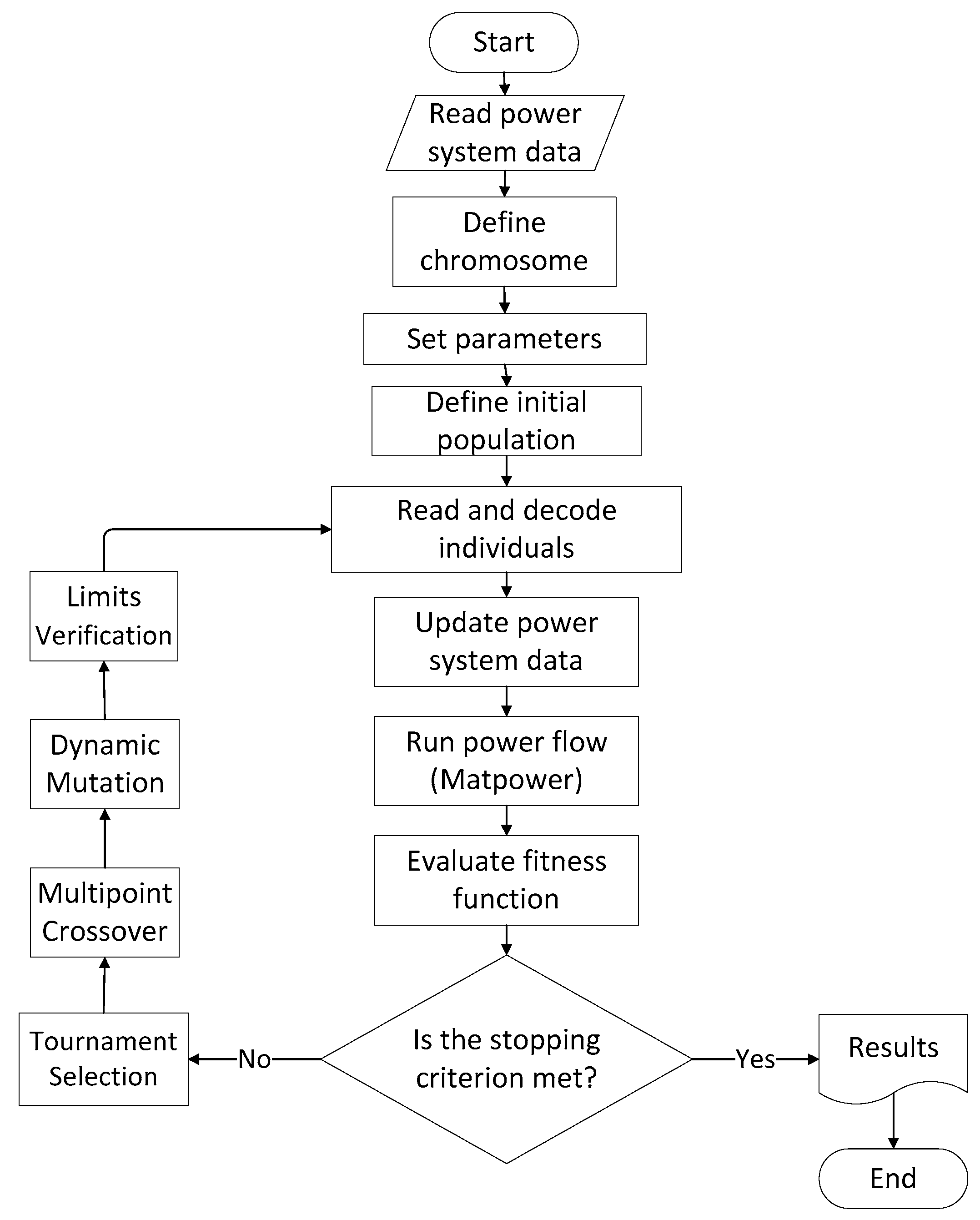
3. Implemented Genetic Algorithm
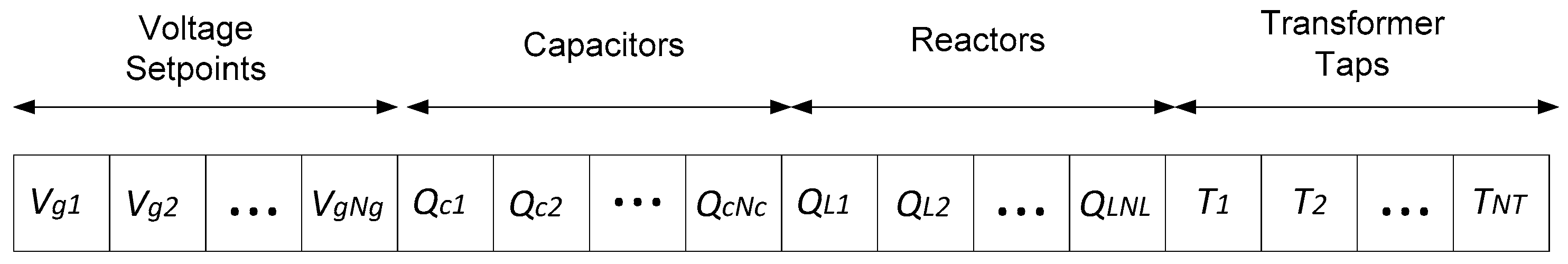
3.1. Codification
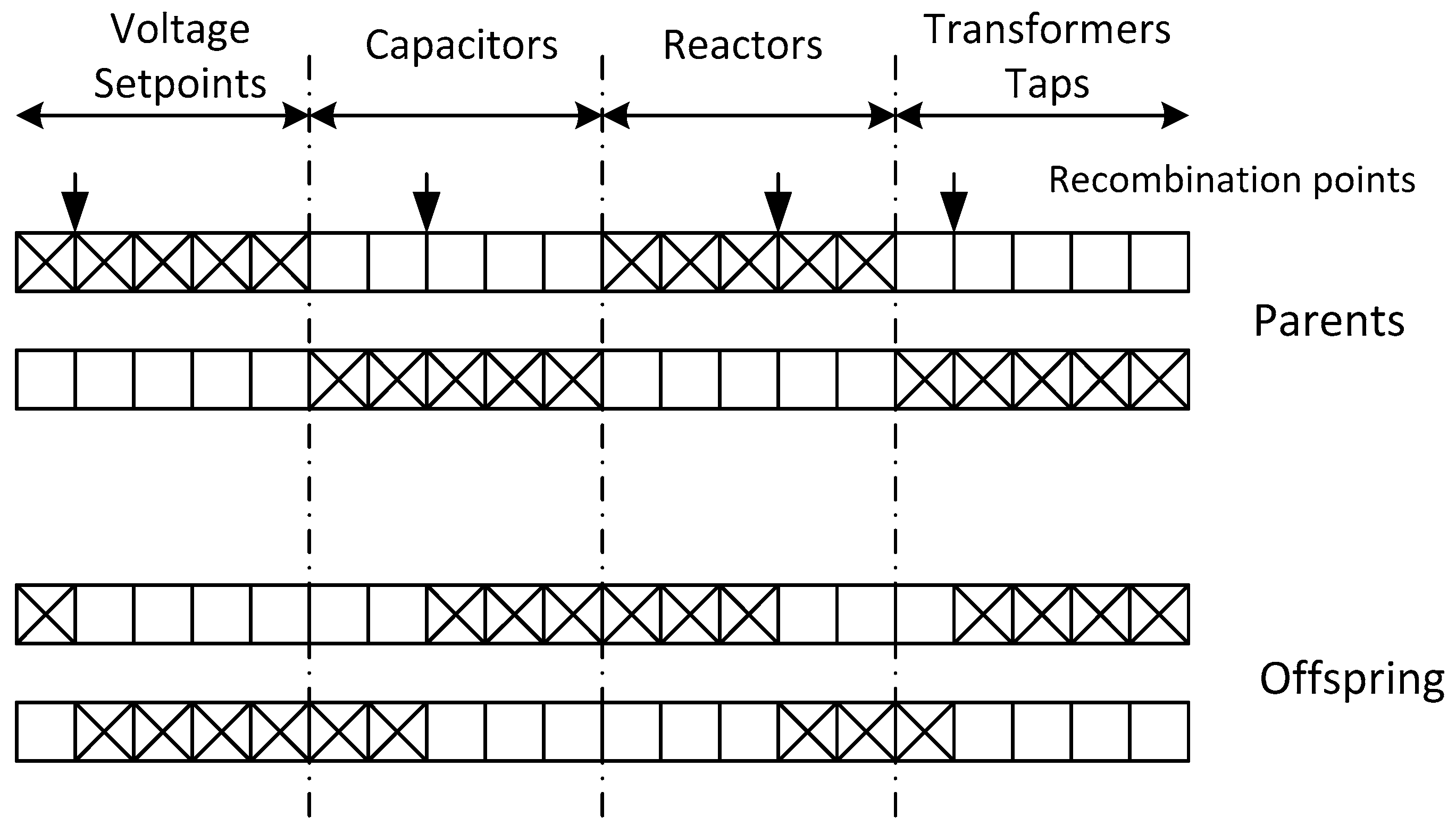
3.2. GA Operators
3.3. Constraint Handling Approaches
3.3.1. Traditional Penalty Function Approach
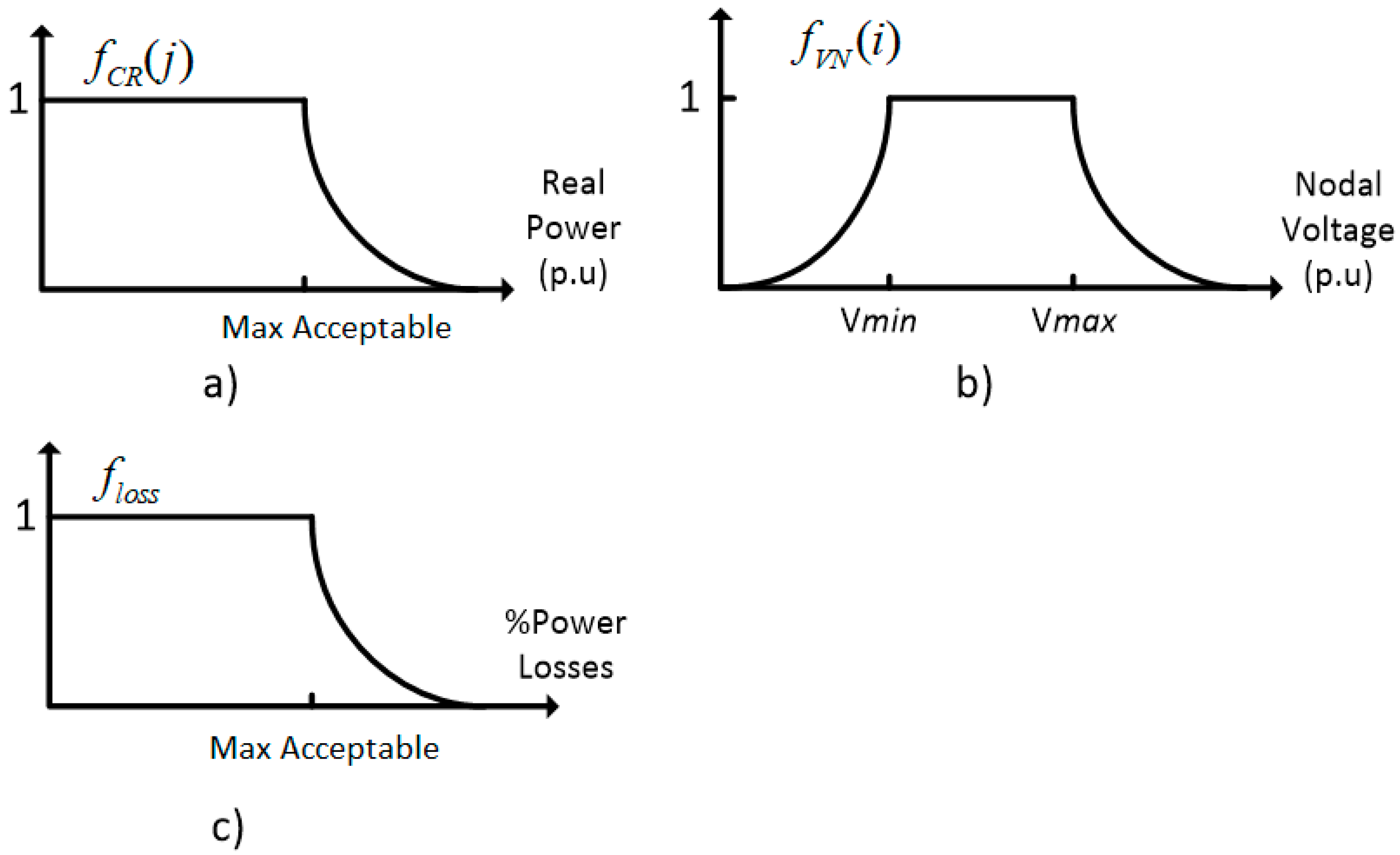
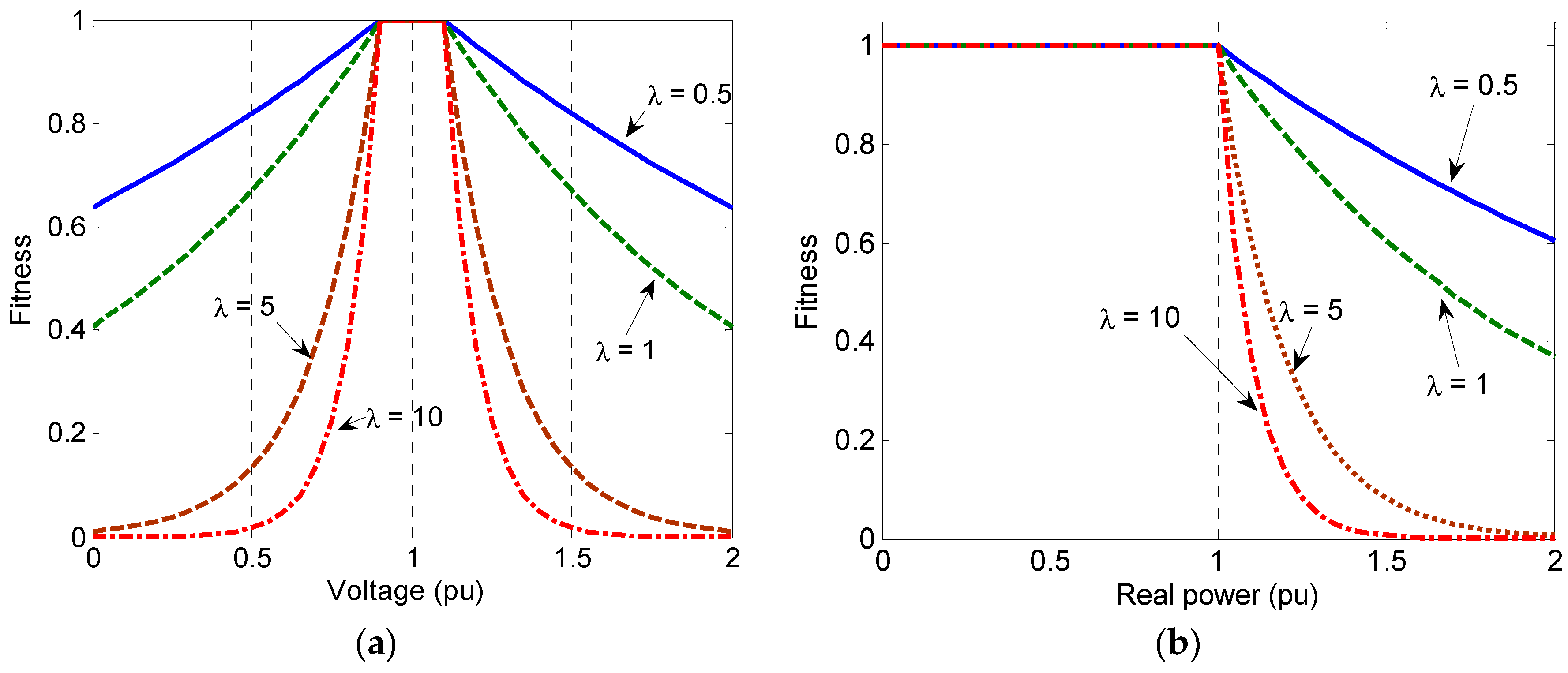
3.3.2. Alternative Constraint Handling Approach
4. Tests and Results
4.1. Input Parameters
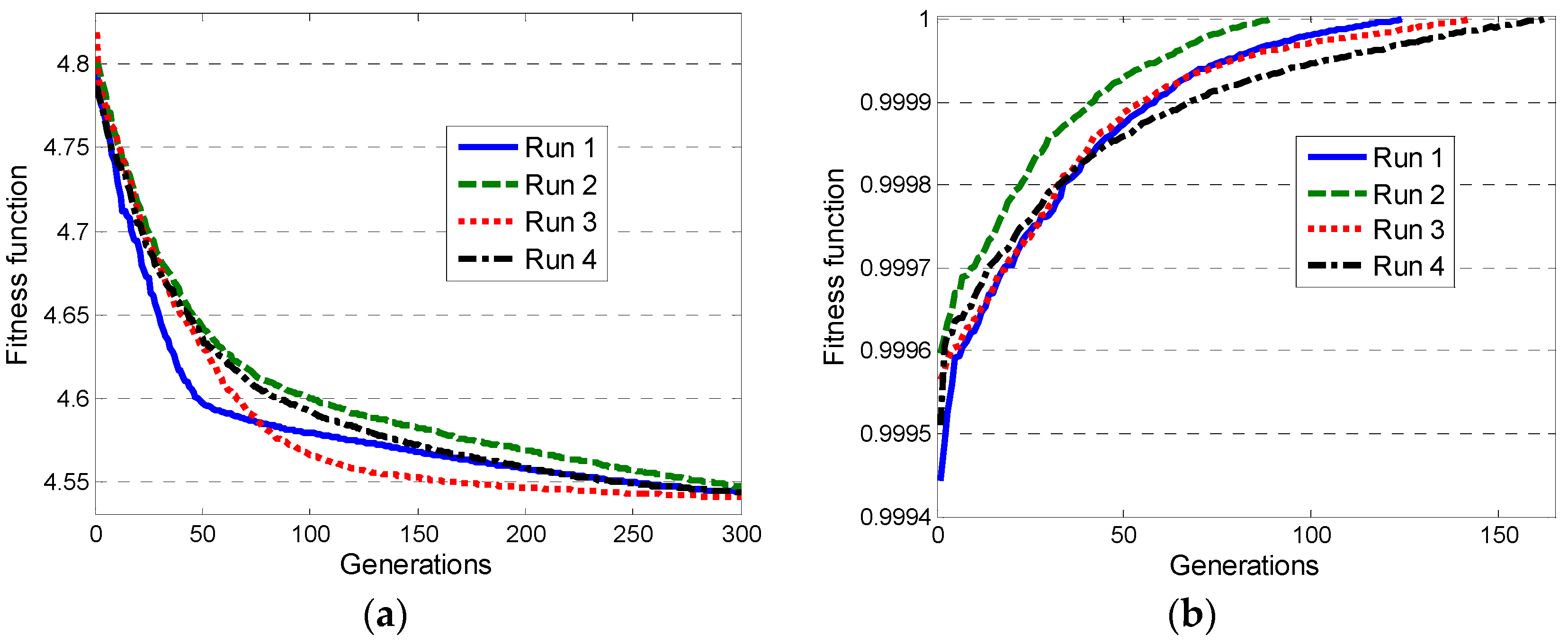
4.2. Results with the IEEE 30 Bus Power System
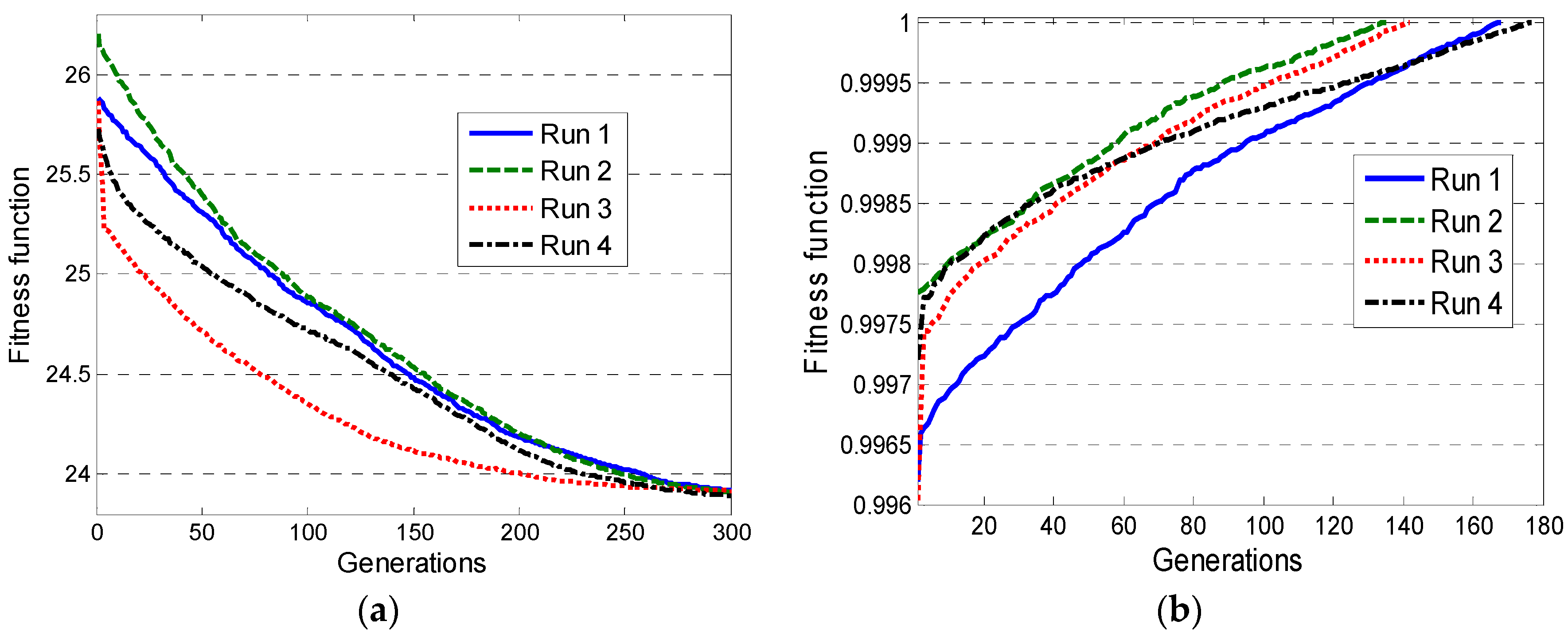
4.3. Results with the IEEE 57 Bus Power System
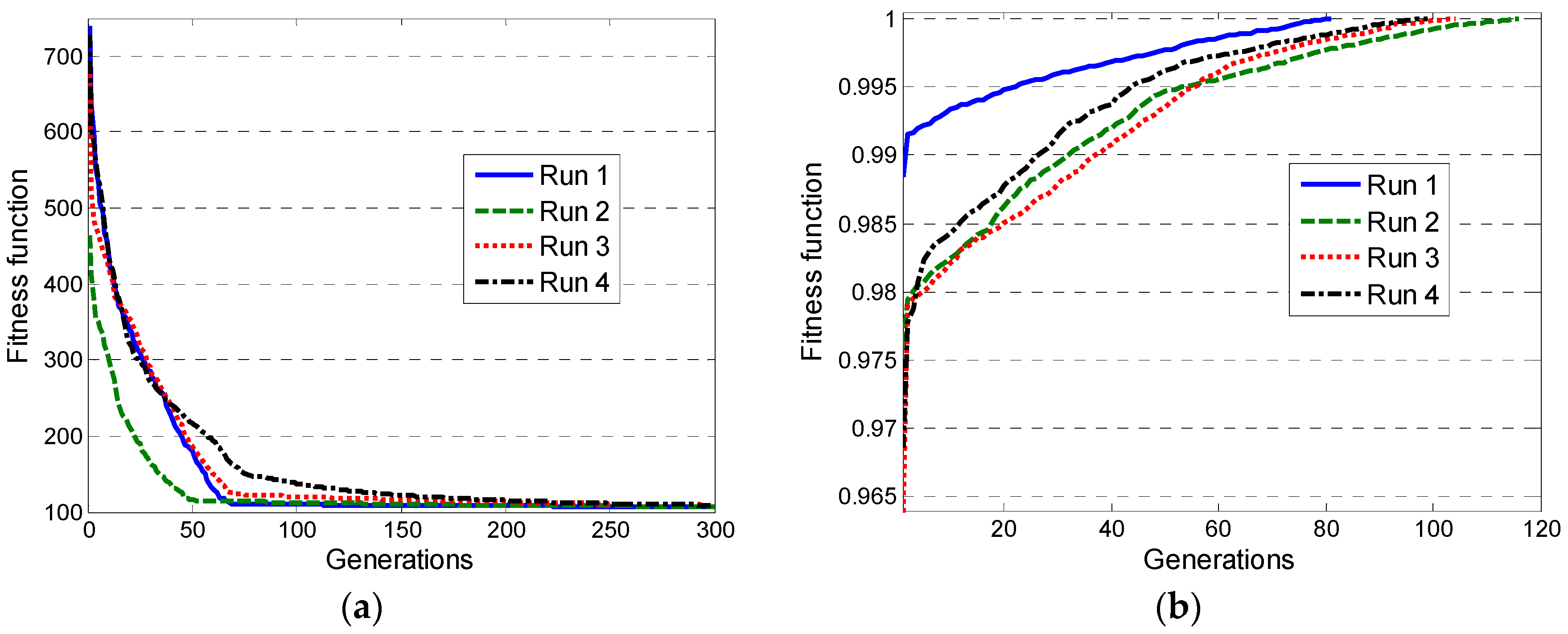
4.4. Results with the IEEE 118 Bus Power System
4.5. Results with the IEEE 300 Bus Power System
4.6. Comparison of Fitness Functions Performance
5. Conclusions
Author Contributions
Acknowledgments
Conflicts of Interest
References
- Lyu, J.-K.; Heo, J.-H.; Park, J.-K.; Kang, Y.-C. Probabilistic Approach to Optimizing Active and Reactive Power Flow in Wind Farms Considering Wake Effects. Energies 2013, 6, 5717–5737. [Google Scholar] [CrossRef]
- Mota-Palomino, R.; Quintana, V.H. Sparse Reactive Power Scheduling by a Penalty Function—Linear Programming Technique. IEEE Trans. Power Syst. 1986, 1, 31–39. [Google Scholar] [CrossRef]
- Lee, K.Y.; Park, Y.M.; Ortiz, J.L. A United Approach to Optimal Real and Reactive Power Dispatch. IEEE Trans. Power Appar. Syst. 1985, PAS-104, 1147–1153. [Google Scholar] [CrossRef]
- Quintana, V.H.; Santos-Nieto, M. Reactive-power dispatch by successive quadratic programming. IEEE Trans. Energy Convers. 1989, 4, 425–435. [Google Scholar] [CrossRef]
- Granville, S. Optimal reactive dispatch through interior point methods. IEEE Trans. Power Syst. 1994, 9, 136–146. [Google Scholar] [CrossRef]
- Bjelogrlic, M.M.; Calovic, S.; Ristanovic, P.; Babic, B.S. Application of Newton’s optimal power flow in voltage/reactive power control. IEEE Trans. Power Syst. 1990, 5, 1447–1454. [Google Scholar] [CrossRef]
- Lu, F.C.; Hsu, Y.Y. Reactive power/voltage control in a distribution substation using dynamic programming. Transm. Distrib. IEE Proc. Gener. 1995, 142, 639–645. [Google Scholar] [CrossRef]
- Aoki, K.; Fan, M.; Nishikori, A. Optimal VAr planning by approximation method for recursive mixed-integer linear programming. IEEE Trans. Power Syst. 1988, 3, 1741–1747. [Google Scholar] [CrossRef]
- Cai, G.; Ren, Z.; Yu, T. Optimal Reactive Power Dispatch Based on Modified Particle Swarm Optimization Considering Voltage Stability. In Proceedings of the 2007 IEEE Power Engineering Society General Meeting, Tampa, FL, USA, 24–28 June 2007. [Google Scholar]
- Kenned, J.; Eberhart, R. Particle swarm optimization. In Proceedings of the International Conference on Neural Networks, Perth, WA, Australia, 27 November–1 December 1995. [Google Scholar]
- Vlachogiannis, J.G.; Lee, K.Y. Determining generator contributions to transmission system using parallel vector evaluated particle swarm optimization. IEEE Trans. Power Syst. 2005, 20, 1765–1774. [Google Scholar] [CrossRef]
- Vlachogiannis, J.G.; Lee, K.Y. A Comparative Study on Particle Swarm Optimization for Optimal Steady-State Performance of Power Systems. IEEE Trans. Power Syst. 2006, 21, 1718–1728. [Google Scholar] [CrossRef]
- Jo, K.-H.; Kim, M.-K. Improved Genetic Algorithm-Based Unit Commitment Considering Uncertainty Integration Method. Energies 2018, 11, 1387. [Google Scholar] [CrossRef]
- Feng, Z.-K.; Niu, W.-J.; Zhou, J.-Z.; Cheng, C.-T.; Qin, H.; Jiang, Z.-Q. Parallel Multi-Objective Genetic Algorithm for Short-Term Economic Environmental Hydrothermal Scheduling. Energies 2017, 10, 163. [Google Scholar] [CrossRef]
- Suresh, R.; Kumarappan, N. Genetic algorithm based reactive power optimization under deregulation. In Proceedings of the 2007 IET-UK International Conference on Information and Communication Technology in Electrical Sciences (ICTES 2007), Tamil Nadu, India, 20–22 December 2007; pp. 150–155. [Google Scholar]
- Vlachogiannis, J.G.; Lee, K.Y. Quantum-Inspired Evolutionary Algorithm for Real and Reactive Power Dispatch. IEEE Trans. Power Syst. 2008, 23, 1627–1636. [Google Scholar] [CrossRef]
- Rueda, J.L.; Erlich, I. Optimal dispatch of reactive power sources by using MVMOs optimization. In Proceedings of the 2013 IEEE Computational Intelligence Applications in Smart Grid (CIASG), Singapore, 16–19 April 2013; pp. 29–36. [Google Scholar]
- Kanna, B.; Singh, S.N. Towards reactive power dispatch within a wind farm using hybrid PSO. Int. J. Electr. Power Energy Syst. 2015, 69, 232–240. [Google Scholar] [CrossRef]
- Rajan, A.; Malakar, T. Optimal reactive power dispatch using hybrid Nelder–Mead simplex based firefly algorithm. Int. J. Electr. Power Energy Syst. 2015, 66, 9–24. [Google Scholar] [CrossRef]
- Amrane, Y.; Boudour, M.; Ladjici, A.A.; Elmaouhab, A. Optimal VAR control for real power loss minimization using differential evolution algorithm. Int. J. Electr. Power Energy Syst. 2015, 66, 262–271. [Google Scholar] [CrossRef]
- Huang, C.M.; Chen, S.J.; Huang, Y.C.; Yang, H.T. Comparative study of evolutionary computation methods for active-reactive power dispatch. Transm. Distrib. IET Gener. 2012, 6, 636–645. [Google Scholar] [CrossRef]
- Rojas, D.G.; Lezama, J.L.; Villa, W. Metaheuristic Techniques Applied to the Optimal Reactive Power Dispatch: A Review. IEEE Lat. Am. Trans. 2016, 14, 2253–2263. [Google Scholar] [CrossRef]
- Mallipeddi, R.; Jeyadevi, S.; Suganthan, P.N.; Baskar, S. Efficient constraint handling for optimal reactive power dispatch problems. Swarm Evol. Comput. 2012, 5, 28–36. [Google Scholar] [CrossRef]
- Singh, R.P.; Mukherjee, V.; Ghoshal, S.P. Optimal reactive power dispatch by particle swarm optimization with an aging leader and challengers. Appl. Soft Comput. 2015, 29, 298–309. [Google Scholar] [CrossRef]
- Mukherjee, A.; Mukherjee, V. Solution of optimal reactive power dispatch by chaotic krill herd algorithm. Transm. Distrib. IET Gener. 2015, 9, 2351–2362. [Google Scholar] [CrossRef]
- Shaw, B.; Mukherjee, V.; Ghoshal, S.P. Solution of reactive power dispatch of power systems by an opposition-based gravitational search algorithm. Int. J. Electr. Power Energy Syst. 2014, 55, 29–40. [Google Scholar] [CrossRef]
- Moharam, R.; Morsy, E. Genetic algorithms to balanced tree structures in graphs. Swarm Evol. Comput. 2017, 32, 132–139. [Google Scholar] [CrossRef]
- López-Lezama, J.M.; Contreras, J.; Padilha-Feltrin, A. Location and contract pricing of distributed generation using a genetic algorithm. Int. J. Electr. Power Energy Syst. 2012, 36, 117–126. [Google Scholar] [CrossRef]
- Zelinka, I. A survey on evolutionary algorithms dynamics and its complexity—Mutual relations, past, present and future. Swarm Evol. Comput. 2015, 25, 2–14. [Google Scholar] [CrossRef]
- López-Lezama, J.M.; Cortina-Gómez, J.; Muñoz-Galeano, N. Assessment of the Electric Grid Interdiction Problem using a nonlinear modeling approach. Electr. Power Syst. Res. 2017, 144, 243–254. [Google Scholar] [CrossRef]
- Zimmerman, R.D.; Murillo-Sánchez, C.E.; Thomas, R.J. MATPOWER: Steady-State Operations, Planning, and Analysis Tools for Power Systems Research and Education. IEEE Trans. Power Syst. 2011, 26, 12–19. [Google Scholar] [CrossRef]
- Yeniay, Ö. Penalty Function Methods for Constrained Optimization with Genetic Algorithms. Math. Comput. Appl. 2015, 10, 45–56. [Google Scholar] [CrossRef]
- Ramirez, J.M.; Marin, G.A. Alleviating congestion of an actual power system by genetic algorithms. In Proceedings of the 2004 IEEE Power Engineering Society General Meeting, Denver, CO, USA, 6–10 June 2004; pp. 2133–2141. [Google Scholar]
- Alsac, O.; Stott, B. Optimal Load Flow with Steady-State Security. IEEE Trans. Power Appar. Syst. 1974, PAS-93, 745–751. [Google Scholar] [CrossRef]
- Ela, A.A.A.E.; Abido, M.A.; Spea, S.R. Differential evolution algorithm for optimal reactive power dispatch. Electr. Power Syst. Res. 2011, 81, 458–464. [Google Scholar] [CrossRef]
- Power Systems Test Case Archive-UWEE. Available online: http://www2.ee.washington.edu/research/pstca/ (accessed on 4 March 2017).
- Mahadevan, K.; Kannan, P.S. Comprehensive learning particle swarm optimization for reactive power dispatch. Appl. Soft Comput. 2010, 10, 641–652. [Google Scholar] [CrossRef]
- Bhattacharya, A.; Chattopadhyay, P.K. Biogeography-Based Optimization for solution of Optimal Power Flow problem. In Proceedings of the 2010 ECTI International Conference on Electrical Engineering/Electronics, Computer, Telecommunications and Information Technology, Chiang Mai, Thailand, 19–21 May 2010; pp. 435–439. [Google Scholar]
- Duman, S.; Sonmez, Y.; Guvenc, U.; Yorukeren, N. Optimal reactive power dispatch using a gravitational search algorithm. Transm. Distrib. IET Gener. 2012, 6, 563–576. [Google Scholar] [CrossRef]
- Ng Shin Mei, R.; Sulaiman, M.H.; Mustaffa, Z.; Daniyal, H. Optimal reactive power dispatch solution by loss minimization using moth-flame optimization technique. Appl. Soft Comput. 2017, 59, 210–222. [Google Scholar] [CrossRef]
- Chen, G.; Liu, L.; Zhang, Z.; Huang, S. Optimal reactive power dispatch by improved GSA-based algorithm with the novel strategies to handle constraints. Appl. Soft Comput. 2017, 50, 58–70. [Google Scholar] [CrossRef]
- Naderi, E.; Narimani, H.; Fathi, M.; Narimani, M.R. A novel fuzzy adaptive configuration of particle swarm optimization to solve large-scale optimal reactive power dispatch. Appl. Soft Comput. 2017, 53, 441–456. [Google Scholar] [CrossRef]
- Heidari, A.A.; Ali Abbaspour, R.; Rezaee Jordehi, A. Gaussian bare-bones water cycle algorithm for optimal reactive power dispatch in electrical power systems. Appl. Soft Comput. 2017, 57, 657–671. [Google Scholar] [CrossRef]
- Dai, C.; Chen, W.; Zhu, Y.; Zhang, X. Seeker Optimization Algorithm for Optimal Reactive Power Dispatch. IEEE Trans. Power Syst. 2009, 24, 1218–1231. [Google Scholar]


| Characteristic | IEEE 30 | IEEE 57 | IEEE 118 | IEEE 300 |
|---|---|---|---|---|
| # buses | 30 | 57 | 118 | 300 |
| # load buses | 24 | 50 | 64 | 231 |
| # generators | 6 | 7 | 54 | 69 |
| # transformers | 4 | 15 | 9 | 107 |
| # capacitors | 9 | 3 | 12 | 8 |
| # reactors | 0 | 0 | 2 | 6 |
| # branches | 41 | 80 | 186 | 411 |
| # Control variables | 19 | 25 | 77 | 190 |
| Base case Ploss (MW) | 5.833 | 27.864 | 132.863 | 408.316 |
| Base case TVD (pu) | 0.58217 | 1.23358 | 1.439337 | 5.4286 |
| Parameter | Value |
|---|---|
| Population size | 60 |
| Maximum number of generations | 300 |
| Mutation rate (transformers taps) | 20% |
| Mutation rate (rest of the chromosome) | 5% |
| Individuals used in tournament selection | 20 |
| IEEE Case | Current Power Losses (MW) | Goal on System Power Losses | |
|---|---|---|---|
| (% Total Gen) | (MW) | ||
| 30 | 5.833 | 1.58 | 4.57 |
| 57 | 27.864 | 2.55 | 23.69 |
| 118 | 132.863 | 2.61 | 108.55 |
| 300 | 408.316 | 1.57 | 368.63 |
| IEEE Case | ||||||||||
|---|---|---|---|---|---|---|---|---|---|---|
| 30 | 1.1 | 0.95 | 0.9 | 1.05 | 0.05 | 0 | 0.0005 | - | - | - |
| 57 | 1.1 | 0.95 | 0.9 | 1.1 | 0.10 | 0 | 0.001 | - | - | - |
| 118 | 1.1 | 0.95 | 0.9 | 1.1 | 0.20 | 0 | 0.001 | −0.40 | 0 | 0.002 |
| 300 | 1.1 | 0.95 | 0.9 | 1.1 | 3.25 | 0 | 0.05 | −3.00 | 0 | 0.05 |
| (a) | |||||||
| Control Variable | Initial [35] | ABC [19] | FA [19] | CLPSO [37] | DE [35] | BBO [38] | HFA [19] |
| , pu | 1.05 | 1.1 | 1.1 | 1.1 | 1.1 | 1.1 | 1.1 |
| , pu | 1.04 | 1.0615 | 1.0644 | 1.1 | 1.0931 | 1.0944 | 1.054332 |
| , pu | 1.01 | 1.0711 | 1.07455 | 1.0795 | 1.0736 | 1.0749 | 1.075146 |
| , pu | 1.01 | 1.0849 | 1.0869 | 1.1 | 1.0736 | 1.0768 | 1.086885 |
| , pu | 1.05 | 1.1 | 1.09164 | 1.1 | 1.1 | 1.0999 | 1.1 |
| , pu | 1.05 | 1.0665 | 1.099 | 1.1 | 1.1 | 1.0999 | 1.1 |
| , pu | 1.078 | 0.97 | 1 | 0.9154 | 1.0465 | 1.0435 | 0.980051 |
| , pu | 1.069 | 1.05 | 0.94 | 0.9 | 0.9097 | 0.90117 | 0.950021 |
| , pu | 1.032 | 0.99 | 1 | 0.9 | 0.9867 | 0.98244 | 0.970171 |
| , pu | 1.068 | 0.99 | 0.97 | 0.9397 | 0.9689 | 0.96918 | 0.970039 |
| , pu | 0 | 5 | 3 | 4.9265 | 5 | 4.9998 | 4.700304 |
| , pu | 0 | 5 | 4 | 5 | 5 | 4.9870 | 4.706143 |
| , pu | 0 | 5 | 3.3 | 5 | 5 | 4.9906 | 4.700662 |
| , pu | 0 | 5 | 3.5 | 5 | 5 | 4.9970 | 2.305910 |
| , pu | 0 | 4.1 | 3.9 | 5 | 4.406 | 4.9901 | 4.803520 |
| , pu | 0 | 3.3 | 3.2 | 5 | 5 | 4.9946 | 4.902598 |
| , pu | 0 | 0.9 | 1.3 | 5 | 2.8004 | 3.8753 | 4.804034 |
| , pu | 0 | 5 | 3.5 | 5 | 5 | 4.9867 | 4.805296 |
| , pu | 0 | 2.4 | 1.42 | 5 | 2.5979 | 2.9098 | 3.398351 |
| , MW | 5.811 | 4.8149 | 4.7694 | 4.6018 | 4.5417 | 4.5435 | 4.7530 |
| TVD, pu | 1.1501 | 1.6815 | 1.9542 | 4.1671 | 1.9737 | 2.0662 | 2.3333 |
| , pu | 0.0097 | 0 | 0 | 1.4560 | 2.220 × 10⁻¹⁶ | 0 | 0.0061 |
| , pu | 0 | 0 | 0 | 0 | 0 | 0 | 0 |
| (b) | |||||||
| Control Variable | GSA [39] | MFO [40] | IGSA-CSS [41] | FAHLCPSO [42] | |||
| pu | 1.071652 | 1.1000 | 1.081281 | 1.1000 | 1.1000 | 1.1000 | |
| pu | 1.022199 | 1.0943 | 1.072177 | 1.0387 | 1.0940 | 1.0970 | |
| pu | 1.040094 | 1.0747 | 1.050142 | 1.0161 | 1.0745 | 1.0805 | |
| pu | 1.050721 | 1.0766 | 1.050234 | 1.0290 | 1.0767 | 1.0835 | |
| pu | 0.977122 | 1.1000 | 1.100000 | 1.0123 | 1.1000 | 1.1000 | |
| pu | 0.967650 | 1.1000 | 1.068826 | 1.1000 | 1.1000 | 1.1000 | |
| , pu | 1.098450 | 1.0433 | 1.0800 | 1.0223 | 1.0510 | 1.0680 | |
| pu | 0.982481 | 0.9000 | 0.9020 | 0.9107 | 0.9000 | 0.9080 | |
| pu | 1.095909 | 0.97912 | 0.9900 | 1.0098 | 0.9830 | 0.9990 | |
| pu | 1.059339 | 0.96474 | 0.9760 | 0.9744 | 0.9670 | 0.9750 | |
| pu | 1.653790 | 0.0500 | 0.0000 | 0.034125 | 0.0500 | 0.0420 | |
| pu | 4.372261 | 0.0500 | 0.0000 | 0.0500 | 0.0500 | 0.0235 | |
| pu | 0.119957 | 0.048055 | 0.0380 | 0.020981 | 0.0500 | 0.0445 | |
| pu | 2.087617 | 0.0500 | 0.0490 | 0.0500 | 0.0500 | 0.0480 | |
| pu | 0.357729 | 0.040263 | 0.0395 | 0.035512 | 0.0435 | 0.0290 | |
| pu | 0.260254 | 0.0500 | 0.0500 | 0.040005 | 0.0500 | 0.0455 | |
| pu | 0.000000 | 2.5193 | 0.0275 | 0.031928 | 0.0270 | 0.0370 | |
| pu | 1.383953 | 0.0500 | 0.0500 | 0.048800 | 0.0500 | 0.0465 | |
| pu | 0.000317 | 0.021925 | 0.0240 | 0.021000 | 0.0240 | 0.0135 | |
| MW | 5.5372 | 4.5410 | 4.7620 | 6.8230 | 4.5399 | 4.5692 | |
| pu | 1.6552 | 2.0316 | 1.1487 | 0.7914 | 2.0105 | 1.8333 | |
| , pu | 0 | 0 | 0 | 0 | 0 | 0 | |
| , pu | 0 | 0 | 0 | 0 | 0 | 0 | |
| (c) | |||||||
| Control Variable | OGSA [26] | ALC-PSO [24] | KHA [25] | CKHA [25] | NGBWCA [43] | ||
| pu | 1.0500 | 1.0500 | 1.0500 | 1.0500 | 1.0502 | 1.0500 | 1.0500 |
| pu | 1.0410 | 1.0384 | 1.0381 | 1.0473 | 1.0382 | 1.0445 | 1.0445 |
| pu | 1.0154 | 1.0108 | 1.0110 | 1.0293 | 1.0107 | 1.0245 | 1.0240 |
| pu | 1.0267 | 1.0210 | 1.0250 | 1.0350 | 1.0212 | 1.0265 | 1.0260 |
| pu | 1.0082 | 1.0500 | 1.0500 | 1.0500 | 1.0503 | 1.0500 | 1.0500 |
| pu | 1.0500 | 1.0500 | 1.0500 | 1.0500 | 1.0500 | 1.0500 | 1.0500 |
| pu | 1.0585 | 0.9521 | 0.9541 | 0.9916 | 0.9520 | 1.0500 | 1.0490 |
| pu | 0.9089 | 1.0299 | 1.0412 | 0.9538 | 1.0295 | 0.9000 | 0.9000 |
| pu | 1.0141 | 0.9721 | 0.9514 | 0.9603 | 0.9720 | 0.9880 | 0.9880 |
| pu | 1.0182 | 0.9657 | 0.9541 | 0.9670 | 0.9661 | 0.9660 | 0.9650 |
| pu | 0.0330 | 0.0090 | 0.0089 | 0.0092 | 0.0097 | 0.0500 | 0.0500 |
| pu | 0.0249 | 0.0126 | 0.0000 | 0.0000 | 0.0125 | 0.0500 | 0.0500 |
| pu | 0.0177 | 0.0209 | 0.0141 | 0.0153 | 0.0212 | 0.0500 | 0.0500 |
| pu | 0.0500 | 0.0500 | 0.04989 | 0.0497 | 0.0541 | 0.0500 | 0.0500 |
| pu | 0.0334 | 0.0031 | 0.0314 | 0.0302 | 0.0043 | 0.0500 | 0.0500 |
| pu | 0.0403 | 0.0293 | 0.0345 | 0.0500 | 0.0289 | 0.0500 | 0.0500 |
| pu | 0.0269 | 0.0226 | 0.0241 | 0.0134 | 0.0229 | 0.0360 | 0.0360 |
| pu | 0.0500 | 0.0500 | 0.0500 | 0.0500 | 0.0498 | 0.0500 | 0.0500 |
| pu | 0.0194 | 0.0107 | 0.0107 | 0.0121 | 0.0106 | 0.0280 | 0.0275 |
| MW | 5.5192 | 5.4711 | 5.5407 | 5.4285 | 5.4720 | 5.0272 | 5.0272 |
| pu | 0.8540 | 0.3001 | 0.2963 | 0.3524 | 0.3003 | 0.7369 | 0.7372 |
| , pu | 0 | 0 | 0 | 0 | 5 × 10⁻⁴ | 0 | 0 |
| , pu | 0 | 0 | 0 | 0 | 0 | 0 | 0 |
| (a) | ||||||||
| Control Variable | Initial [35] | SOA [44] | CLPSO [39] | DE [44] | BBO [39] | ALC-PSO [24] | MFO [40] | NGBWCA [43] |
| pu | 1.0400 | 1.0541 | 1.0541 | 1.0397 | 1.0600 | 1.0600 | 1.06000 | 1.0600 |
| pu | 1.0100 | 1.0529 | 1.0529 | 1.0463 | 1.0504 | 1.0593 | 1.05870 | 1.0591 |
| pu | 0.9850 | 1.0337 | 1.0337 | 1.0511 | 1.0440 | 1.0491 | 1.04690 | 1.0492 |
| pu | 0.9800 | 1.0313 | 1.0313 | 1.0236 | 1.0376 | 1.0432 | 1.04210 | 1.0399 |
| pu | 1.0500 | 1.0496 | 1.0496 | 1.0538 | 1.0550 | 1.0600 | 1.06000 | 1.0586 |
| pu | 0.9800 | 1.0302 | 1.0302 | 0.9451 | 1.0229 | 1.0451 | 1.04230 | 1.0461 |
| pu | 1.0150 | 1.0302 | 1.0342 | 0.9907 | 1.0323 | 1.0411 | 1.03730 | 1.0413 |
| pu | 0.9700 | 0.9900 | 0.9900 | 1.0200 | 0.9669 | 0.9611 | 0.95011 | 0.9712 |
| pu | 0.9780 | 0.9800 | 0.9800 | 0.9100 | 0.9902 | 0.9109 | 1.00760 | 0.9243 |
| pu | 1.0430 | 0.9900 | 0.9900 | 0.9700 | 1.0120 | 0.9000 | 1.00630 | 0.9123 |
| pu | 1.0430 | 1.0100 | 1.0100 | 0.9100 | 1.0087 | 0.9004 | 1.00760 | 0.9001 |
| pu | 0.9670 | 0.9900 | 0.9900 | 0.9600 | 0.9707 | 0.9106 | 0.97523 | 0.9112 |
| pu | 0.9650 | 0.9300 | 0.9300 | 0.9900 | 0.9686 | 0.9000 | 0.97218 | 0.9004 |
| pu | 0.9550 | 0.9100 | 0.9100 | 0.9800 | 0.9008 | 0.9000 | 0.90000 | 0.9128 |
| pu | 0.9550 | 0.9700 | 0.9700 | 0.9600 | 0.9660 | 0.9000 | 0.97186 | 0.9000 |
| pu | 0.9000 | 0.9500 | 0.9500 | 1.0500 | 0.9507 | 1.0275 | 0.95355 | 1.0218 |
| pu | 0.9300 | 0.9800 | 0.9800 | 1.0700 | 0.9641 | 0.9876 | 0.96736 | 0.9902 |
| pu | 0.8950 | 0.9500 | 0.9500 | 0.9900 | 0.9246 | 0.9756 | 0.92788 | 0.9568 |
| pu | 0.9580 | 0.9500 | 0.9500 | 1.0600 | 0.9502 | 0.9000 | 0.96406 | 0.9000 |
| pu | 0.9580 | 1.0000 | 1.0000 | 0.9900 | 0.9966 | 0.9000 | 0.99980 | 0.9000 |
| pu | 0.9800 | 0.9600 | 0.9600 | 0.9700 | 0.9628 | 1.0121 | 0.96060 | 1.0118 |
| pu | 0.9400 | 0.9700 | 0.9700 | 1.0700 | 0.9600 | 0.9944 | 0.97899 | 1.0000 |
| pu | 0 | 0.0988 | 0.0988 | 0 | 0.09782 | 0.0994 | 0.099968 | 0.0914 |
| pu | 0 | 0.0542 | 0.0542 | 0 | 0.05899 | 0.0590 | 0.05900 | 0.0587 |
| pu | 0 | 0.0628 | 0.0628 | 0 | 0.06289 | 0.0630 | 0.06300 | 0.0634 |
| pu | 0.2786 | 0.2487 | 0.2489 | 0.3594 | 0.2454 | 0.2618 | 0.242529 | 0.2674 |
| TVD, pu | 4.1788 | 1.0775 | 1.0929 | 4.1788 | 1.3548 | 2.2077 | 1.4885 | 2.1427 |
| , pu | 0.7951 | 0 | 0 | 0.7951 | 0 | 0.1428 | 7.29 × 10⁻⁵ | 0.3913 |
| , pu | 0.2948 | 0.0035 | 0.0022 | 0.2948 | 3.49 × 10⁻⁴ | 0.0829 | 0 | 0.0895 |
| (b) | ||||||||
| Control Variable | GSA [39] | OGSA [26] | KHA [25] | CKHA [25] | ||||
| pu | 1.0600 | 1.0600 | 1.0556 | 1.0600 | 1.0600 | 1.0600 | ||
| pu | 1.0600 | 1.0594 | 1.0595 | 1.0590 | 1.0594 | 1.0594 | ||
| pu | 1.0600 | 1.0492 | 1.0414 | 1.0487 | 1.0490 | 1.0523 | ||
| pu | 1.0081 | 1.0433 | 1.0314 | 1.0431 | 1.0418 | 1.0451 | ||
| pu | 1.0549 | 1.0600 | 1.0549 | 1.0600 | 1.0600 | 1.0600 | ||
| pu | 1.009.8 | 1.0450 | 1.0415 | 1.0447 | 1.0435 | 1.0484 | ||
| pu | 1.0185 | 1.0407 | 1.0398 | 1.0410 | 1.0396 | 1.0473 | ||
| pu | 1.1000 | 0.9000 | 0.9211 | 0.9179 | 1.0190 | 1.0130 | ||
| pu | 1.0826 | 0.9947 | 1.0214 | 1.0256 | 0.9130 | 1.0040 | ||
| pu | 0.9219 | 0.9000 | 0.9912 | 0.9000 | 1.0320 | 1.0580 | ||
| pu | 1.0167 | 0.9001 | 0.9119 | 0.9020 | 1.0070 | 1.0200 | ||
| pu | 0.9962 | 0.9111 | 0.9101 | 0.9104 | 0.9410 | 0.9670 | ||
| pu | 1.1000 | 0.9000 | 0.9946 | 0.9005 | 0.9780 | 0.9930 | ||
| pu | 1.0746 | 0.9000 | 0.9457 | 0.9000 | 0.9100 | 1.0370 | ||
| pu | 0.9543 | 0.9000 | 0.9914 | 0.9000 | 0.9380 | 0.9430 | ||
| pu | 0.9377 | 1.0464 | 1.0714 | 1.0797 | 0.9250 | 0.9480 | ||
| pu | 1.0167 | 0.9875 | 0.9945 | 0.9887 | 0.9350 | 0.9660 | ||
| pu | 1.0525 | 0.9638 | 0.9814 | 0.9914 | 0.9030 | 0.9250 | ||
| pu | 1.1000 | 0.9000 | 0.9715 | 0.9000 | 0.9260 | 0.9660 | ||
| pu | 0.9799 | 0.9000 | 0.9001 | 0.9002 | 1.0140 | 0,9950 | ||
| pu | 1.0246 | 1.0148 | 1.0136 | 1.0173 | 0.9740 | 1.0380 | ||
| pu | 1.0373 | 0.9830 | 1.0089 | 1.0023 | 0.9430 | 0.9840 | ||
| pu | 0.0782 | 0.0682 | 0.0894 | 0.0994 | 0.0510 | 0.0970 | ||
| pu | 0.0058 | 0.0590 | 0.0459 | 0.0590 | 0.0570 | 0.0580 | ||
| pu | 0.0468 | 0.0630 | 0.0625 | 0.0630 | 0.0630 | 0.0435 | ||
| pu | 0.2940 | 0.2642 | 0.2618 | 0.2748 | 0.23836 | 0.24325 | ||
| TVD, pu | 2.8536 | 2.1764 | 2.4490 | 2.2741 | 2.7021 | 1.7616 | ||
| , pu | 0.4369 | 0.1036 | 0.0851 | 0.0818 | 0 | 0 | ||
| , pu | 0.0483 | 0.0948 | 0.0107 | 0.1445 | 9.9 × 10⁻⁷ | 0 | ||
| (a) | |||||||||
| Control Variable | MFO [40] | NGBWCA [43] | FAHCLPSO [42] | Control Variable | MFO [40] | NGBWCA [43] | FAHCLPSO [42] | ||
| pu | 1.0173 | 1.0215 | 1.0120 | pu | 1.0496 | 0.9989 | 1.0298 | ||
| pu | 1.0402 | 1.0431 | 1.0523 | pu | 1.0600 | 1.0001 | 1.1005 | ||
| pu | 1.0292 | 1.0312 | 1.0666 | pu | 1.0551 | 1.0467 | 1.0498 | ||
| pu | 1.0600 | 1.0539 | 1.0597 | pu | 1.0584 | 1.0213 | 1.0565 | ||
| pu | 1.0374 | 1.0271 | 1.0725 | pu | 1.0442 | 1.0416 | 1.0413 | ||
| pu | 1.0250 | 1.0316 | 1.0333 | pu | 1.0333 | 1.0174 | 1.0189 | ||
| pu | 1.0268 | 1.0129 | 1.0012 | pu | 1.0281 | 1.0223 | 1.1000 | ||
| pu | 1.0298 | 1.0075 | 1.0058 | pu | 1.0161 | 1.0340 | 1.0222 | ||
| pu | 1.0275 | 1.0102 | 1.1000 | pu | 1.0215 | 1.0103 | 1.0115 | ||
| pu | 1.0483 | 1.0208 | 1.0971 | pu | 1.0280 | 1.0345 | 1.1000 | ||
| pu | 1.0600 | 1.0531 | 1.0899 | pu | 1.0042 | 1.0160 | 1.0500 | ||
| pu | 1.0600 | 0.9941 | 1.1000 | pu | 1.0350 | 1.0181 | 1.0099 | ||
| pu | 1.0267 | 1.0291 | 1.0654 | pu | 1.0484 | 1.0330 | 1.0500 | ||
| pu | 1.0101 | 1.0275 | 1.0318 | pu | 1.01360 | 1.0051 | 1.0214 | ||
| pu | 1.0226 | 1.0201 | 1.0322 | pu | 1.10000 | 0.9614 | 1.0533 | ||
| pu | 1.0556 | 1.0014 | 0.9999 | pu | 1.00380 | 0.9961 | 1.0555 | ||
| pu | 1.0548 | 1.0412 | 0.9998 | pu | 0.98263 | 0.9523 | 0.9995 | ||
| pu | 1.0419 | 1.0400 | 1.0501 | pu | 0.98430 | 1.0521 | 1.0619 | ||
| pu | 1.0429 | 1.0512 | 1.0231 | pu | 1.01390 | 0.9520 | 1.0318 | ||
| pu | 1.0450 | 1.0170 | 1.0005 | pu | 1.10000 | 0.9812 | 1.0490 | ||
| pu | 1.0589 | 1.0510 | 0.9897 | pu | 1.10000 | 0.9510 | 0.9660 | ||
| pu | 1.0284 | 1.0392 | 0.9998 | pu | 0.96831 | 0.9754 | 0.9732 | ||
| pu | 1.0289 | 1.0331 | 1.0222 | pu | 0 | −0.0723 | 0.0035 | ||
| pu | 1.0283 | 1.0372 | 1.0008 | pu | 0 | 0.0483 | 0.101922 | ||
| pu | 1.0512 | 1.0564 | 1.0731 | pu | −0.03126 | −0.2390 | 0.017500 | ||
| pu | 1.0534 | 1.0565 | 1.0258 | pu | 0.10 | 0.0032 | 0.04400 | ||
| pu | 1.0506 | 1.0489 | 1.0059 | pu | 0 | 0.0372 | 0.069894 | ||
| pu | 1.0596 | 1.0435 | 1.0630 | pu | 0 | 0.0624 | 0.071289 | ||
| pu | 1.0600 | 1.0435 | 1.0312 | pu | 0.000842 | 0.0172 | 0.066668 | ||
| pu | 1.0600 | 1.0489 | 1.0636 | pu | 0.022054 | 0.0013 | 0.110952 | ||
| pu | 1.0600 | 1.0113 | 1.1000 | pu | 0.20 | 0.0621 | 0.15000 | ||
| pu | 1.0526 | 1.0382 | 1.0500 | pu | 0 | 0.0463 | 0.105509 | ||
| pu | 1.0600 | 0.9926 | 1.0981 | pu | 0.10 | 0.0560 | 0.055540 | ||
| pu | 1.0600 | 0.9934 | 1.0444 | pu | 0 | 0.0653 | 0.151895 | ||
| pu | 1.0390 | 1.0324 | 1.0037 | pu | 0.06 | 0.0072 | 0.044140 | ||
| pu | 1.0502 | 1.0185 | 1.0559 | pu | 0.06 | 0.0108 | 0.022310 | ||
| pu | 1.0600 | 1.0021 | 0.9999 | pu | 1.164254 | 1.2147 | 1.162479 | ||
| pu | 1.0600 | 1.0312 | 1.0882 | TVD, pu | 2.3416 | 1.452 | 2.5204 | ||
| pu | 1.0599 | 1.0212 | 1.0303 | , pu | 0 | 0 | 0 | ||
| pu | 1.0600 | 1.0387 | 1.0001 | ,pu | 0 | 0 | 0 | ||
| pu | 1.0431 | 1.0071 | 1.0018 | ||||||
| (b) | |||||||||
| Control Variable | ALC-PSO [24] | GSA [39] | Control Variable | ALC-PSO [24] | GSA [39] | ||||
| pu | 1.0218 | 0.9600 | 1.0880 | 1.0947 | pu | 0.9997 | 1.0032 | 1.0955 | 1.0985 |
| pu | 1.0432 | 0.9620 | 1.1000 | 1.1000 | pu | 1.0012 | 1.0927 | 1.0993 | 1.0992 |
| pu | 1.0224 | 0.9729 | 1.0963 | 1.0970 | pu | 1.0481 | 1.0433 | 1.0955 | 1.0992 |
| pu | 1.0543 | 1.0570 | 1.0828 | 1.0820 | pu | 1.0332 | 1.0786 | 1.1000 | 1.1000 |
| pu | 1.0901 | 1.0885 | 1.0910 | 1.0895 | pu | 1.0422 | 1.0266 | 1.0993 | 1.0985 |
| pu | 1.0325 | 0.9630 | 1.0940 | 1.0992 | pu | 1.0183 | 0.9808 | 1.0963 | 1.1000 |
| pu | 1.0140 | 1.0127 | 1.0850 | 1.0955 | pu | 1.0226 | 1.0163 | 1.0948 | 1.0985 |
| pu | 1.0080 | 1.0069 | 1.0888 | 1.0947 | pu | 1.0344 | 0.9987 | 1.0895 | 1.1000 |
| pu | 1.0104 | 1.0003 | 1.0850 | 1.0992 | pu | 1.0349 | 1.0218 | 1.0963 | 1.1000 |
| pu | 1.0200 | 1.0105 | 1.0978 | 1.0985 | pu | 1.0425 | 0.9852 | 1.1000 | 1.0977 |
| pu | 1.0551 | 1.0102 | 1.1000 | 1.1000 | pu | 1.0162 | 0.9500 | 1.0835 | 1.0985 |
| pu | 0.9932 | 1.0401 | 1.1000 | 1.0992 | pu | 1.0188 | 0.9764 | 1.0963 | 1.0977 |
| pu | 1.0288 | 0.9809 | 1.0933 | 1.0977 | pu | 1.0331 | 1.0372 | 1.0985 | 1.0992 |
| pu | 1.0288 | 0.9500 | 1.0888 | 1.0977 | pu | 1.0065 | 1.0659 | 0.9920 | 1.0000 |
| pu | 1.0248 | 0.9552 | 1.0895 | 1.0970 | pu | 0.9617 | 0.9534 | 1.0450 | 1.0110 |
| pu | 1.0362 | 0.9910 | 1.0940 | 1.0887 | pu | 0.9745 | 0.9328 | 0.9870 | 1.0050 |
| pu | 1.0407 | 1.0091 | 1.0940 | 1.0925 | pu | 0.9404 | 1.0884 | 0.9790 | 0.9500 |
| pu | 1.0391 | 0.9505 | 1.0843 | 1.0955 | pu | 1.0531 | 1.0579 | 0.9800 | 0.9550 |
| pu | 1.0507 | 0.9500 | 1.0873 | 1.0985 | pu | 0.9539 | 0.9493 | 1.0040 | 0.9990 |
| pu | 1.0171 | 0.9814 | 1.0903 | 1.1000 | pu | 0.9448 | 0.9975 | 0.9960 | 1.0730 |
| pu | 1.0492 | 1.0444 | 1.1000 | 1.1000 | pu | 0.9502 | 0.9887 | 0.9600 | 0.9720 |
| pu | 1.0424 | 1.0379 | 1.0903 | 1.0992 | pu | 0.9747 | 0.9801 | 0.9840 | 0.9800 |
| pu | 1.0339 | 0.9907 | 1.0903 | 1.0992 | pu | −0.0075 | 0.0000 | −0.0050 | −0.0020 |
| pu | 1.0393 | 1.0333 | 1.0888 | 1.0992 | pu | 0.0677 | 0.0746 | 0.0500 | 0.0160 |
| pu | 1.0585 | 1.0099 | 1.1000 | 1.1000 | pu | −0.2399 | 0.0000 | −0.0050 | 0.000 |
| pu | 1.0569 | 1.0925 | 1.0993 | 1.0992 | pu | 0.0038 | 0.0604 | 0.0145 | 0.0890 |
| pu | 1.0491 | 1.0393 | 1.0948 | 1.0977 | pu | 0.0179 | 0.0333 | 0.0025 | 0.0270 |
| pu | 1.0437 | 0.9998 | 1.1000 | 1.0992 | pu | 0.0780 | 0.0651 | 0.0155 | 0.0470 |
| pu | 1.0716 | 1.0355 | 1.1000 | 1.0992 | pu | 0.0789 | 0.0447 | 0.0350 | 0.0040 |
| pu | 1.0535 | 1.1000 | 1.1000 | 1.1000 | pu | 0.0000 | 0.0972 | 0.0005 | 0.1070 |
| pu | 1.0111 | 1.0992 | 1.0880 | 1.0985 | pu | 0.0717 | 0.1425 | 0.0190 | 0.0220 |
| pu | 1.0389 | 1.0014 | 1.0955 | 1.1000 | pu | 0.0589 | 0.1749 | 0.0470 | 0.0650 |
| pu | 0.9932 | 1.0111 | 1.0955 | 1.0977 | pu | 0.0561 | 0.0428 | 0.0025 | 0.0020 |
| pu | 0.9912 | 1.0476 | 1.0775 | 1.0940 | pu | 0.0641 | 0.1204 | 0.0005 | 0.1860 |
| pu | 1.0335 | 1.0211 | 1.0768 | 1.0805 | pu | 0.0000 | 0.0226 | 0.0380 | 0.0135 |
| pu | 1.0191 | 1.0187 | 1.0895 | 1.09475 | pu | 0.0110 | 0.0294 | 0.0130 | 0.0495 |
| pu | 1.0247 | 1.0462 | 1.0993 | 1.1000 | pu | 1.2153 | 1.2776 | 1.0633 | 1.0846 |
| pu | 1.0324 | 1.0491 | 1.1000 | 1.0992 | TVD, pu | 1.4651 | 2.2243 | 5.5245 | 5.7253 |
| pu | 1.0243 | 1.0426 | 1.0985 | 1.0970 | , pu | 0 | 0 | 0 | 0 |
| pu | 1.0303 | 1.0955 | 1.1000 | 1.1000 | , pu | 0 | 0 | 0 | 0 |
| pu | 1.0072 | 1.0417 | 1.0910 | 1.0985 | |||||
| Control Variable | Initial | Control Variable | Initial | Control Variable | Initial | ||||||
|---|---|---|---|---|---|---|---|---|---|---|---|
| pu | 1.0153 | 1.0887 | 1.0962 | pu | 1.0000 | 1.0992 | 1.0985 | pu | 0.9565 | 1.0520 | 1.0080 |
| pu | 1.0205 | 1.0962 | 1.0992 | pu | 1.0000 | 1.0985 | 1.0940 | pu | 1.0000 | 0.9270 | 0.9160 |
| pu | 1.0010 | 1.0910 | 1.0925 | pu | 1.0000 | 1.0955 | 1.1000 | pu | 1.050 | 0.9860 | 1.0150 |
| pu | 0.9583 | 1.1000 | 1.0970 | pu | 1.0000 | 1.0977 | 1.0977 | pu | 1.0730 | 1.0430 | 1.0010 |
| pu | 0.9632 | 1.0775 | 1.0587 | pu | 1.0082 | 1.0480 | 0.9690 | pu | 1.0500 | 0.9260 | 0.9960 |
| pu | 1.0250 | 1.0962 | 1.0985 | pu | 0.9668 | 0.9310 | 1.0480 | pu | 1.0506 | 1.0250 | 0.9230 |
| pu | 1.0520 | 1.1000 | 1.0970 | pu | 0.9796 | 1.0380 | 1.0520 | pu | 0.9750 | 0.9240 | 1.0260 |
| pu | 1.0520 | 1.0992 | 1.0992 | pu | 1.0435 | 1.0050 | 1.0190 | pu | 0.9800 | 0.9480 | 0.9720 |
| pu | 1.0000 | 1.0985 | 1.0985 | pu | 0.9391 | 0.9370 | 0.9970 | pu | 0.9560 | 0.9970 | 0.9910 |
| pu | 0.9900 | 1.0842 | 1.0940 | pu | 1.0435 | 1.0130 | 0.9970 | pu | 1.0500 | 1.0080 | 1.0080 |
| pu | 1.0435 | 1.0992 | 1.1000 | pu | 1.0435 | 1.0140 | 1.0460 | pu | 1.0300 | 0.9390 | 1.0520 |
| pu | 1.0233 | 1.0992 | 1.0985 | pu | 1.0435 | 0.9610 | 1.0550 | pu | 1.0300 | 1.0230 | 1.0850 |
| pu | 1.0103 | 1.0692 | 1.0992 | pu | 1.0000 | 0.9790 | 0.9780 | pu | 0.9850 | 1.0200 | 0.9920 |
| pu | 1.0550 | 1.1000 | 1.0940 | pu | 1.0000 | 1.0080 | 1.0240 | pu | 1.0000 | 1.0330 | 1.0190 |
| pu | 1.0510 | 1.0985 | 1.0992 | pu | 1.0000 | 1.0850 | 1.0790 | pu | 1.0300 | 0,9850 | 0.9360 |
| pu | 1.0435 | 1.1000 | 1.0977 | pu | 1.0000 | 1.0620 | 1.0320 | pu | 1.0100 | 0,9260 | 1.0110 |
| pu | 1.0528 | 1.0962 | 1.0985 | pu | 1.0000 | 0.9750 | 0.9780 | pu | 1.0500 | 1.0560 | 1.0800 |
| pu | 1.0528 | 1.0992 | 1.0970 | pu | 1.0000 | 1.0810 | 1.0760 | pu | 1.0300 | 1.0150 | 0.9920 |
| pu | 1.0735 | 1.0895 | 1.0970 | pu | 1.0000 | 0.9980 | 1.0620 | pu | 1.0000 | 1.0340 | 1.0380 |
| pu | 1.0535 | 1.0137 | 1.0962 | pu | 1.0000 | 0.9560 | 1.0690 | pu | 0.9700 | 1.0010 | 0.9990 |
| pu | 1.0435 | 1.0962 | 1.0970 | pu | 1.0000 | 0.9210 | 1.0110 | pu | 1.0000 | 1.0300 | 1.0480 |
| pu | 0.9630 | 1.0977 | 1.0962 | pu | 1.0000 | 0.9960 | 1.0040 | pu | 1.0200 | 0.9590 | 0.9940 |
| pu | 0.9290 | 1.0955 | 1.0970 | pu | 1.0000 | 0.9790 | 0.9790 | pu | 1.0700 | 0.9750 | 1.0470 |
| pu | 0.9829 | 1.1000 | 1.1000 | pu | 1.0000 | 0.9910 | 0.9140 | pu | 1.0200 | 1.0000 | 0.9890 |
| pu | 1.0522 | 1.1000 | 1.0992 | pu | 1.0000 | 0.9710 | 1.0890 | pu | 1.0000 | 1,0460 | 1.0370 |
| pu | 1.0077 | 1.0985 | 1.0992 | pu | 1.0000 | 1.0950 | 1.0830 | pu | 1.0223 | 1.0080 | 1.0250 |
| pu | 1.0522 | 1.0992 | 1.0977 | pu | 1.0000 | 0.9380 | 1.0130 | pu | 0.9284 | 0.9800 | 0.9320 |
| pu | 1.0650 | 1.0992 | 1.0955 | pu | 1.0000 | 1.0700 | 1.0880 | pu | 1.0000 | 0.9970 | 0.9890 |
| pu | 1.0650 | 1.0985 | 1.0940 | pu | 1.0000 | 1.0290 | 1.0710 | pu | 1.0000 | 0.9080 | 1.0890 |
| pu | 1.0551 | 1.0857 | 1.0842 | pu | 0.9583 | 1.0050 | 0.9980 | pu | 1.0000 | 1.0530 | 0.9390 |
| pu | 1.0435 | 1.1000 | 1.0970 | pu | 1.0000 | 0.9760 | 0.9830 | pu | 0.95 | 0.9320 | 1.0580 |
| pu | 1.0150 | 1.0992 | 1.0955 | pu | 1.0000 | 0.9620 | 1.0960 | pu | 1.0000 | 1.0130 | 1.0740 |
| pu | 1.0100 | 1.0992 | 1.0992 | pu | 1.0000 | 1.0220 | 1.0270 | pu | 1.0000 | 1.0000 | 1.0190 |
| pu | 1.0080 | 1.0940 | 1.0947 | pu | 1.0000 | 1.0830 | 1.0120 | pu | 1.0000 | 1.0270 | 0.9540 |
| pu | 1.0000 | 1.0970 | 1.0992 | pu | 0.9470 | 1.0460 | 1.0240 | pu | 1.0000 | 1.0110 | 0.9990 |
| pu | 1.0500 | 1.0947 | 1.0962 | pu | 0.9560 | 0.9400 | 0.9750 | pu | 1.0000 | 1.0200 | 0.9930 |
| pu | 1.0000 | 1.0992 | 1.1000 | pu | 0.9710 | 0.9970 | 0.9550 | pu | 1.0000 | 1.0020 | 1.0240 |
| pu | 1.0400 | 1.0985 | 1.0662 | pu | 0.9480 | 1.0150 | 1.0300 | pu | 1.0000 | 0.9940 | 1.0130 |
| pu | 1.0000 | 1.0947 | 1.0962 | pu | 0.9590 | 1.0120 | 0.9620 | pu | 1.0000 | 0.9770 | 0.9840 |
| pu | 1.0165 | 1.0992 | 1.0985 | pu | 1.0460 | 1.0840 | 1.0400 | pu | 1.0000 | 0.9570 | 0.9880 |
| pu | 1.0100 | 1.0985 | 1.0970 | pu | 0.9850 | 1.0280 | 1.0640 | pu | 0.9420 | 0,9900 | 1.0150 |
| pu | 1.0000 | 1.1000 | 1.0992 | pu | 0.9561 | 0.9790 | 0.9740 | pu | 0.9650 | 0.9980 | 1.0660 |
| pu | 1.0500 | 1.0992 | 1.0970 | pu | 0.9710 | 0.9500 | 0.9210 | pu | 0.9500 | 1,0420 | 1.0590 |
| pu | 0.993 | 1.0962 | 1.0917 | pu | 0.9520 | 0.9960 | 1.0370 | pu | 0.9420 | 0.9740 | 0.9030 |
| pu | 1.0100 | 1.0985 | 1.0985 | pu | 0.9430 | 1.0620 | 0.9400 | pu | 0.9420 | 0.9120 | 1.0650 |
| pu | 1.0507 | 1.0985 | 1.0962 | pu | 1.0100 | 0.9410 | 1.0530 | pu | 0.95650 | 1.0350 | 1.0090 |
| pu | 1.0507 | 1.0992 | 1.1000 | pu | 1.0080 | 0.9770 | 1.0060 | pu | 3.2500 | 1.8000 | 0.8000 |
| pu | 1.0323 | 0.9897 | 1.0940 | pu | 1.0000 | 0.9870 | 0.9850 | pu | 0.5500 | 0.0200 | 0.4800 |
| pu | 1.0145 | 1.1000 | 1.0962 | pu | 0.9750 | 0.9550 | 1.0230 | pu | 0.3450 | 0.0000 | 0.1250 |
| pu | 1.0507 | 1.0955 | 1.0992 | pu | 1.0170 | 0.9970 | 0.9810 | pu | −2.120 | −0.020 | −1.740 |
| pu | 1.0507 | 1.0985 | 1.0992 | pu | 1.0000 | 1.0450 | 1.0820 | pu | −1.030 | 0.0000 | −0.060 |
| pu | 1.0507 | 1.1000 | 1.0977 | pu | 1.0000 | 1.0100 | 0.9690 | pu | 0.5300 | 0.0900 | 0.1950 |
| pu | 1.0290 | 1.0550 | 1.0977 | pu | 1.0000 | 1.0040 | 0.9490 | pu | 0.4500 | 0.1450 | 0.2500 |
| pu | 1.0500 | 1.0977 | 1.0977 | pu | 1.0000 | 1.0130 | 0.9480 | pu | −1.5000 | −0.060 | −0.080 |
| pu | 1.0145 | 1.0977 | 1.0977 | pu | 1.0150 | 1.0000 | 1.0960 | pu | −3.000 | −0.350 | −0.100 |
| pu | 1.0507 | 1.0925 | 1.0977 | pu | 0.9670 | 0.9810 | 1.0580 | pu | −1.500 | −0.080 | −0.040 |
| pu | 0.9967 | 1.0985 | 1.0977 | pu | 1.0100 | 0.9140 | 0.9940 | pu | −1.400 | −0.260 | −0.100 |
| pu | 1.0212 | 1.0992 | 1.0985 | pu | 1.0500 | 0.9540 | 1.0060 | pu | 0.4560 | 0.1450 | 0.1250 |
| pu | 1.0145 | 1.1000 | 1.0962 | pu | 1.0000 | 1.0820 | 1.0250 | pu | 0.0240 | 0.0120 | 0.0500 |
| pu | 1.0017 | 1.0947 | 1.0970 | pu | 1.0522 | 1.0140 | 1.0970 | pu | 0.0172 | 0.0075 | 0.0475 |
| pu | 0.9893 | 1.0992 | 1.1000 | pu | 1.0522 | 1.0060 | 1.0290 | pu | 4.0831 | 3.5710 | 3.6798 |
| pu | 1.0507 | 1.1000 | 1.0985 | pu | 1.0500 | 1.0480 | 1.0150 | TVD, pu | 5.4286 | 15.744 | 15.315 |
| pu | 1.0507 | 1.0992 | 1.0992 | pu | 0.9750 | 0.9910 | 1.0610 | , pu | 0 | 4.77 × 10⁻⁵ | 0 |
| pu | 1.0145 | 1.0940 | 1.0962 | pu | 1.0000 | 0.9180 | 0.9710 | , pu | 0 | 0 | 0 |
| pu | 0.9945 | 1.0962 | 1.0962 | pu | 1.0350 | 1.0510 | 1.0040 |
| IEEE Cases | 30 | 57 | 118 | 300 | ||||
|---|---|---|---|---|---|---|---|---|
| Fitness function | ||||||||
| Best solution, MW | 4.5399 | 4.5692 | 23.8365 | 24.3251 | 106.3394 | 108.4626 | 357.1041 | 367.9837 |
| , pu | 0 | 0 | 0 | 0 | 0 | 0 | 4.77 × 10⁻⁵ | 0 |
| , pu | 0 | 0 | 9.9 × 10⁻⁷ | 0 | 0 | 0 | 0 | 0 |
| Worst solution, MW | 4.5557 | 4.5700 | 24.1669 | 24.3371 | 111.2652 | 108.8013 | 405.4689 | 373.8592 |
| Mean, MW | 4.5448 | 4.5698 | 23.9581 | 24.3345 | 107.4481 | 108.5458 | 371.7911 | 368.5625 |
| Standard deviation | 0.0040 | 1.55 × 10⁻⁴ | 0.0706 | 0.0025 | 1.0389 | 0.0311 | 8.4040 | 0.6314 |
| Success rate, % | - | 100 | - | 100 | - | 100 | - | 97 |
| Average CPU time, s. | 27.1713 | 13.7408 | 34.4150 | 16.4009 | 40.3389 | 17.8228 | 77.4805 | 61.0231 |
© 2018 by the authors. Licensee MDPI, Basel, Switzerland. This article is an open access article distributed under the terms and conditions of the Creative Commons Attribution (CC BY) license (http://creativecommons.org/licenses/by/4.0/).
Share and Cite
Villa-Acevedo, W.M.; López-Lezama, J.M.; Valencia-Velásquez, J.A. A Novel Constraint Handling Approach for the Optimal Reactive Power Dispatch Problem. Energies 2018, 11, 2352. https://doi.org/10.3390/en11092352
Villa-Acevedo WM, López-Lezama JM, Valencia-Velásquez JA. A Novel Constraint Handling Approach for the Optimal Reactive Power Dispatch Problem. Energies. 2018; 11(9):2352. https://doi.org/10.3390/en11092352
Chicago/Turabian StyleVilla-Acevedo, Walter M., Jesús M. López-Lezama, and Jaime A. Valencia-Velásquez. 2018. "A Novel Constraint Handling Approach for the Optimal Reactive Power Dispatch Problem" Energies 11, no. 9: 2352. https://doi.org/10.3390/en11092352
APA StyleVilla-Acevedo, W. M., López-Lezama, J. M., & Valencia-Velásquez, J. A. (2018). A Novel Constraint Handling Approach for the Optimal Reactive Power Dispatch Problem. Energies, 11(9), 2352. https://doi.org/10.3390/en11092352