A Pressure-Coordinated Control for Vehicle Electro-Hydraulic Braking Systems

1
State Key Laboratory of Mechanical Transmission, Chongqing University, Chongqing 400044, China
2
School of Automotive Engineering, Chongqing University, Chongqing 400044, China
3
College of Mechanical Engineering, Chongqing University, Chongqing 400044, China
*
Author to whom correspondence should be addressed.
Energies 2018, 11(9), 2336; https://doi.org/10.3390/en11092336
Submission received: 25 July 2018
/
Revised: 25 August 2018
/
Accepted: 27 August 2018
/
Published: 4 September 2018
Abstract
:The characteristics of electro-hydraulic braking systems have a direct influence on the fuel consumption, emissions, brake safety, and ride comfort of hybrid electric vehicles. In order to realize efficient energy recovery for ensuring braking safety and considering that the existing electro-hydraulic braking pressure control systems have control complexity disadvantages and functional limitations, this study considers the front and rear dual-motor-driven hybrid electric vehicle as the prototype and based on antilock brake system (ABS) hardware, proposes a new braking pressure coordinated control system with electro-hydraulic braking function and developed a corresponding control strategy in order to realize efficient energy recovery and ensure braking safety, while considering the disadvantages of control complexity and functional limitations of existing electro-hydraulic system. The system satisfies the pressure coordinated control requirements of conventional braking, regenerative braking, and ABS braking. The vehicle dynamics model based on braking control strategy and pressure coordinated control system is established, and thereafter, the performance simulation of the vehicle-based pressure coordinated control system under typical braking conditions is carried out to validate the performance of the proposed system and control strategy. The simulation results show that the braking energy recovery rates under three different conditions—variable braking intensity, constant braking intensity and integrated braking model—are 66%, 55% and 47%. The battery state of charge (SOC) recovery rates are 0.37%, 0.31% and 0.36%. This proves that the motor can recover the reduced energy of the vehicle during braking and provide an appropriate braking force. It realizes the ABS control function and has good dynamic response and braking pressure control accuracy. The simulation results illustrate the effectiveness and feasibility of the program which lays the foundation for further design and optimization of the new regenerative braking system.
1. Introduction
Hybrid electric vehicles (HEVs) meet can satisfy the comprehensive requirements of low emissions and low fuel consumption, and as one of the most important fuel-saving technologies of HEVs, regenerative braking can save vehicle energy and reduce emissions significantly [1,2,3].
The electro-hydraulic braking system of hybrid electric vehicles consists of the regenerative braking system (motor braking system), vehicle hydraulic braking system, and engine braking system [4]. Hence, the braking process of hybrid electric vehicles is a dynamic process which is influenced by a synthesis of multiple parameters and multi-system interactions. The characteristics of electro-hydraulic braking systems have a direct influence on the fuel consumption, emissions, braking safety, and ride comfort of hybrid electric vehicles.
At present, the studies on electro-hydraulic braking system mainly focus on the formulation of braking force distribution strategies and the design of the braking systems. Fujimoto et al. studied a braking force distribution model that considered the acceleration and speed of the vehicle to optimize the distribution of braking force [5]. Hernández et al. found an optimized braking distribution between axles and between regenerative and friction braking to reach the target of a highly efficiency electric braking [6]. Itani et al. made a comparison of the braking force distribution method of wheel slip ratio control based on the robust sliding mode controller and the braking force distribution method based on the constraint of ECE. The simulation results showed that the energy recovery efficiency of ECE-based allocation method is higher under medium and high friction pavement [7]. Toyota designed a system that regulates wheel-cylinder pressure by adjusting a linear solenoid valve current based on the Electronic Hydraulic Brake (EHB) system; the system can simulate the feel of a braking pedal and satisfy the pressure requirement during electro-hydraulic braking [8]. For the control strategy of electro-hydraulic composite braking system, Ko et al. considered the braking force between the tire and road, and increased the friction braking force of the rear wheel according to the friction coefficient. Finally they designed a control algorithm for the regenerative braking of the front wheel [9]. In the actual braking process of the electro-hydraulic composite braking, the maximum regenerative braking torque provided by the motor cannot meet the needs of some forced working conditions. Therefore, the regenerative braking needs to cooperate with the hydraulic braking to ensure braking safety and braking stability [10]. Generally speaking, the characteristic of regenerative braking is the rapid response, while the hydraulic braking is characterized by response hysteresis. Therefore, due to the different dynamic characteristics of regenerative braking and traditional hydraulic braking, there is always a significant change or mutation of the braking torque when the braking mode is switched [11]. Some scholars have studied the brake-by-wire system in which the existing hydraulic system is replaced by motor-driven electro-mechanical calipers; this system has the advantages of quick response and high flexibility, however, this system cannot be widely used in vehicles because of its high cost and some implementation difficulties [12,13].
Braking pressure control of hybrid electric vehicles is critical to realize the braking force distribution strategy. Traditional braking systems cannot meet the electro-hydraulic braking requirements of hybrid electric vehicles. Furthermore, the configuration of existing HEV braking systems is complicated, and does not fully utilize the existing ABS hardware to realize ABS-based pressure coordinated control. Advanced electro-hydraulic braking systems and good integrated control strategies is some of the problems that must be solved in the process of electric vehicle production. Therefore, the design of an efficient electro-hydraulic composite braking system, a new braking force distribution strategy and pressure coordination control method can greatly improve the contribution of regenerative braking to the improvement of overall vehicle fuel economy.
In this study, taking a plug-in hybrid electric vehicle driven by front and rear axle double motors as the research object, based on the functional requirements of the brake system and based on the ABS hardware, a new braking force control strategy is proposed to ensure braking safety and maximize the braking energy recovery, and subsequently, a braking pressure coordinated control system is designed. By simulating the system under variable-strength braking, constant-strength braking, conventional braking, ABS braking, and integrated braking, the system braking force control strategy and the dynamic performance of the braking pressure coordinated control system are verified. The simulation verified the validity of the braking force control strategy and pressure coordinated control system.
2. Electro-Hydraulic Braking System Structure and Braking Force Control Strategy
2.1. Structure and Function Design of the Braking System
The braking system is designed based on the traditional vehicle ABS hardware. This system can achieve pressure coordinated braking in addition to conventional braking with the advantages of requiring only slight modification and low cost. The schematic diagram of a hybrid electro-hydraulic braking system is shown in Figure 1. The vehicle collects gathers the signals of braking pedal displacement, vehicle speed, continuously variable transmission (CVT) ratio, battery state of charge (SOC), and other signals through the controller area network (CAN) bus, and subsequently calculates the required motor braking force and hydraulic braking force. The required motor and hydraulic braking force signals are sent to the Hydraulic Control Unit (HCU) and Motor Control Unit (MCU) for braking force control through the CAN bus. The main parameters of the vehicle are listed in Table 1.
2.2. Braking Force Control Strategy of Pressure Coordinated Control System
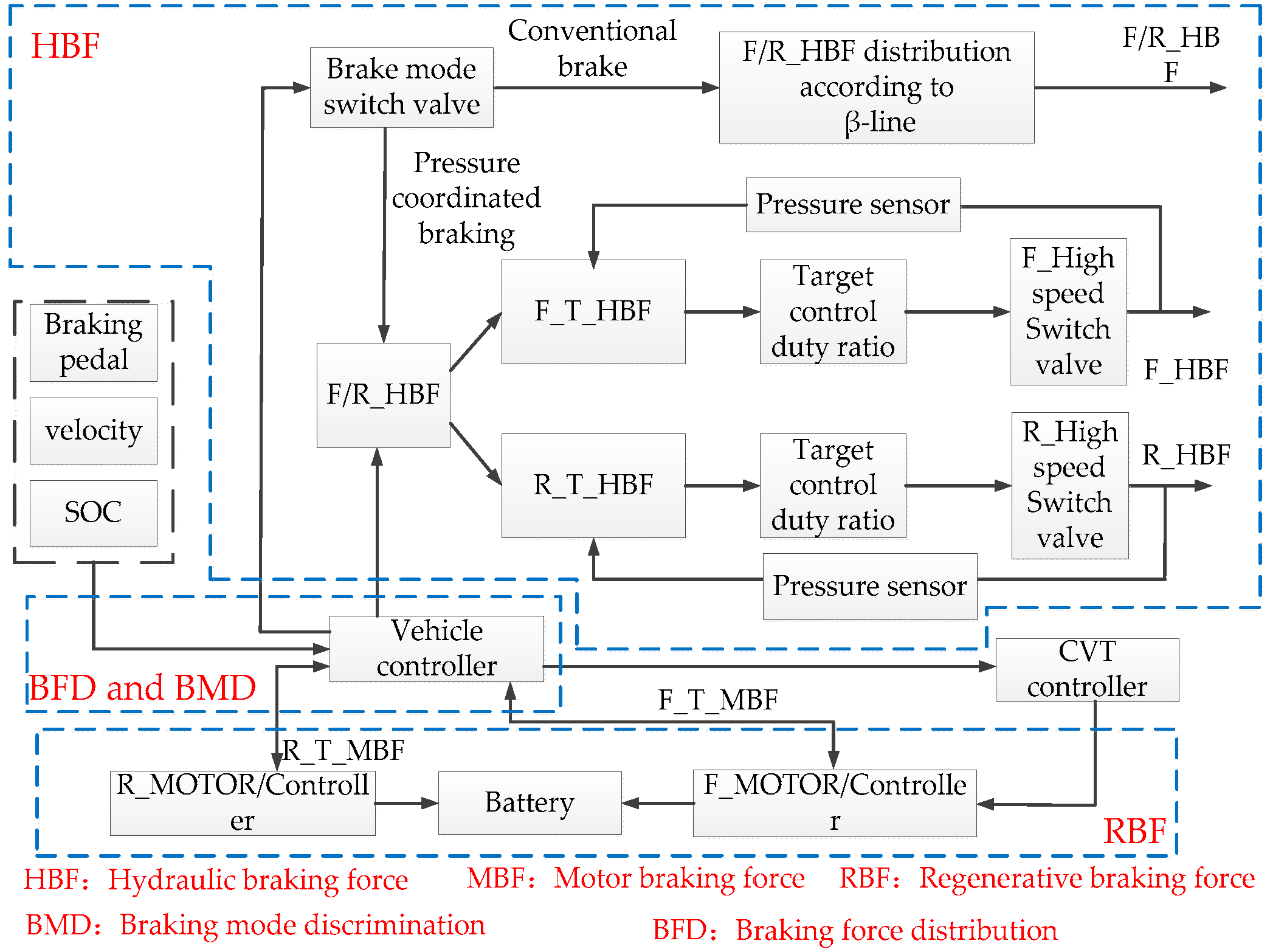
The system braking modes include conventional braking and regenerative braking. The control flowchart of the braking system is shown in Figure 2, where and denote the maximum braking forces of the front and rear motors, respectively, denotes the required braking force.
When the emergency braking is applied, the vehicle speed is too low, or the battery is not suitable for charging, the system works in conventional braking mode; thus, the braking force is only provided by the master cylinder, and the front and rear axle hydraulic braking forces are distributed in accordance with the traditional -line ( denotes the braking force distribution coefficient. -line denotes the braking force distribution curve of front and rear brakes) as shown in Equation (1).
where denotes the total required braking force, denotes the front axle hydraulic braking force, denotes the rear axle hydraulic braking force, denotes the braking strength, and .
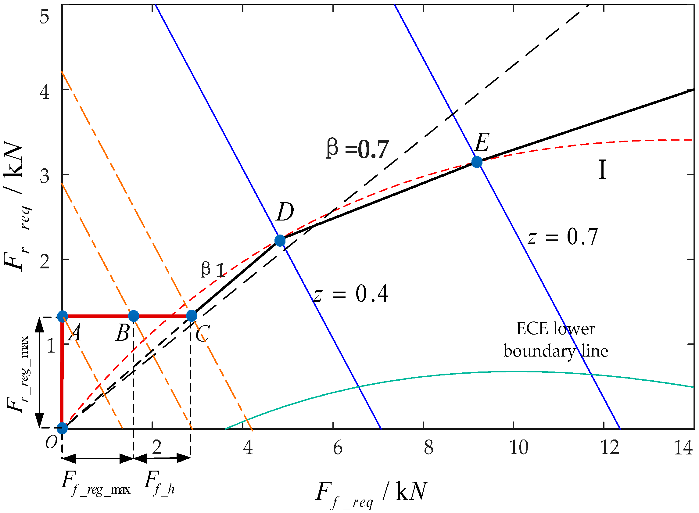
When none of the above conditions is satisfied, the system works in regenerative braking mode. The regenerative braking system attempts to maximize the energy recovery rate under the premise of ensuring braking safety [14]. The braking force distribution strategy has an important influence on the energy recovery rate of the regenerative braking system. Considering that the hybrid electric vehicle has two motors and the transmission efficiency of the rear axle is higher than that of the front axle, the braking force is provided priority by the rear motor, the remaining part is provided by the front motor. In addition, the front motor braking force can be magnified by adjusting the CVT ratio so that the front motor braking force can be fully utilized. When the front and rear motor braking force is insufficient, the hydraulic braking force is added as a supplement.
The distribution of braking force is shown in Figure 3, where and denote the required braking forces of the front and rear axles, respectively, O is the origin of coordinates, the point A denotes the maximum braking forces of the rear motors, the point B denotes the maximum braking forces of the rear and front motors, point C is the rear axle hydraulic braking force starting to take part in braking, the point D is the intersection of line z = 0.4 and curve I, and the point E is the intersection of line z = 0.7 and curve I. The intersection point of the I curve and the equal braking intensity curve with z = 0.4 and z = 0.7 is used as the connection point of the braking force distribution curve, so that the braking force distribution curve is as close as possible to the I curve, thereby ensuring the safety of the braking. As shown in Figure 3, when the system operates in regenerative braking mode, the braking strengths of A, B, and C are:
where denotes the ratio of the front axle braking force to the total required braking force, which is determined by the slope of OD.
2.3. Electro-Hydraulic Braking Pressure Coordinated Control Strategy
The detailed braking force control of the electro-hydraulic braking system is shown in Figure 4.
When the driver depresses the braking pedal, the vehicle controller obtains the braking pedal signal, vehicle speed signal, and SOC signal to determine the braking mode and thereafter operates the pressure coordinated control system in the traditional braking mode or pressure coordinated braking mode by controlling the mode switch valve. When the system is operated in the conventional braking mode, the front and rear axle hydraulic braking forces are distributed in accordance with the traditional -line and the motor does not apply the brake. When the system is operated in the regenerative braking mode, the vehicle controller calculates the target regenerative braking force and the target hydraulic braking force for the front and rear axles, and thereafter sends them to the corresponding controller. The hydraulic braking force is controlled by adjusting the duty cycle of each high-speed switch valve, and the motor braking force is controlled by the motor controller and CVT controller.
3. Hydraulic Braking System Design and Pressure Control
3.1. Structure Design of Braking System
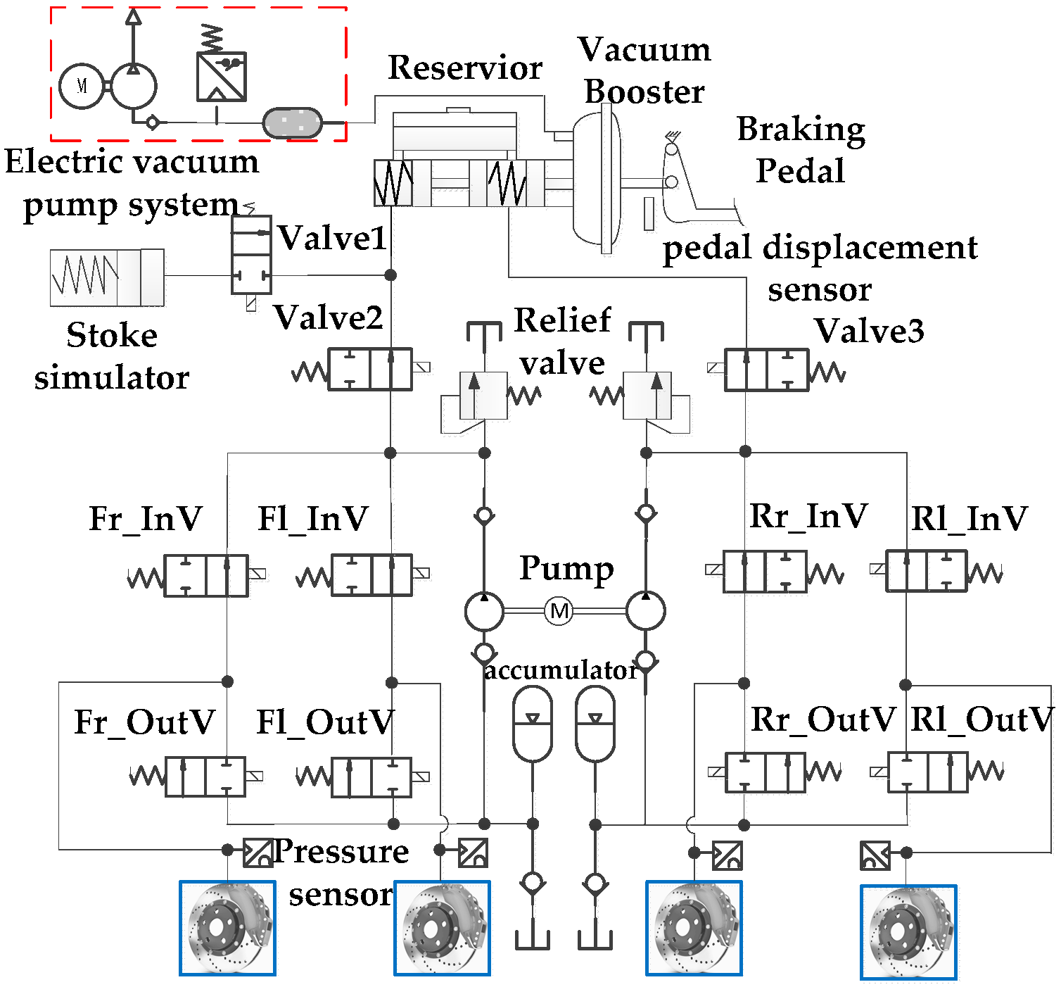
Based on the analysis of the above requirements, a new braking pressure coordinated control system is developed. The designed hydraulic braking system is transformed from the hardware of the traditional ABS braking system. As shown in Figure 5, the system mainly includes a braking pedal, pedal displacement sensor, reservoir, vacuum booster system, stroke simulator, wheel cylinder pressure sensor, high-speed switch valve, regulating valve, and reflux pump.
The system can achieve the traditional master cylinder braking and pressure coordinated braking. In the pressure coordinated braking mode, by closing the two normally open valves 2 and 3 and opening the normal closed valve 1, the master cylinder and wheel cylinder are decoupled and the front cavity’s oil of the master cylinder into the stroke simulator which can simulate the feel of a braking pedal. Furthermore, the reflux pump starts pumping oil and the pressure of each wheel cylinder is controlled by a pair of high-speed switch valves among which the inlet valve is normally open, and the outlet valve is normally closed. The error between the actual wheel cylinder pressure and target wheel cylinder pressure is calculated and thereafter inputted to a proportional integral derivative (PID) controller to calculate the duty cycle of the pulse width of each valve to achieve precise control of the wheel cylinder pressure. When the system is operated in the conventional braking mode, the normally closed valve 1 remains closed and the normally open valves 2 and 3 remain open, and the hydraulic pressure of the wheel cylinder is provided by the master cylinder.
Considering the failure of the electronic control unit of the pressure coordinated control system, in the event of a braking system failure, each valve is powered off; thus, InV is open, OutV is closed, the system is operated in the conventional braking mode, and braking pressure is provided by the master cylinder, which guarantees safety. The main parameters of the braking system are listed in Table 2.
3.2. Mathematical Model of High-Speed Switch Valve
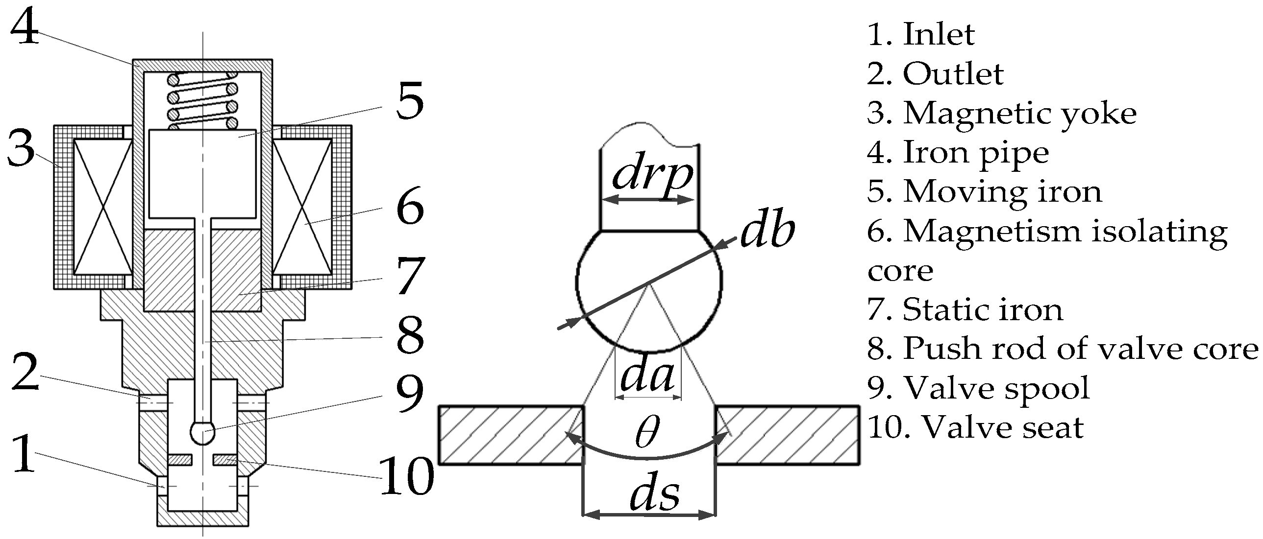
The structure of the normally closed high-speed switch valve is shown in Figure 6. It consists of an inlet, outlet, magnetic yoke, iron pipe, moving iron, magnetism isolating core, static iron, push rod of valve core, valve spool, and valve seat. During its operation, the turn-on and turn-off of the switch valve is achieved by controlling its current [15].
The kinematic equation of the high-speed switch valve under electromagnetic force is:
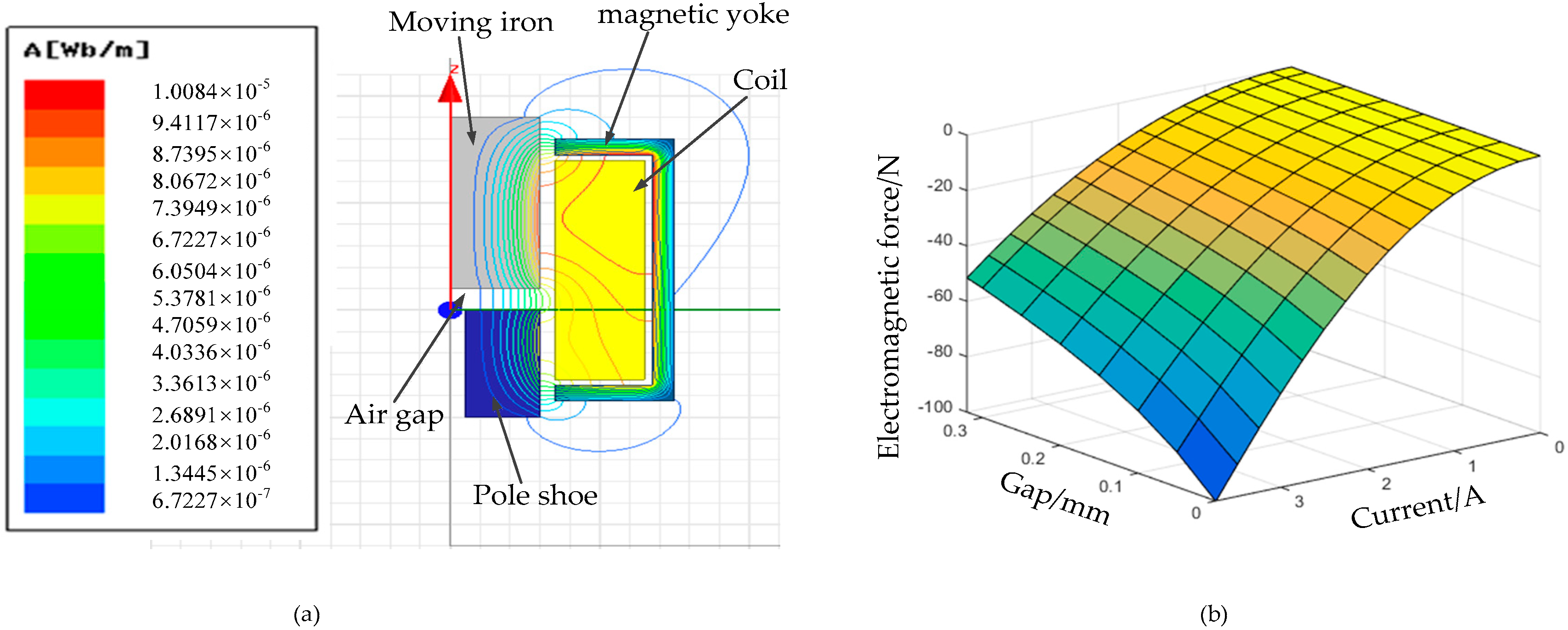
where m denotes the total mass of the moving iron and push rod of the valve core, and denote the electromagnetic force and frictional force, respectively, denotes the stiffness of the return spring, denotes the hydraulic force of the valve core assembly, denotes the impact force, denotes the velocity viscosity coefficient, denotes the pre-compression force of the return spring, and denotes the displacement of the valve core. The structure of the electromagnet of the high-speed switch valve is shown in Figure 7a.
It is mainly composed of a moving iron, pole shoe, coil, magnetic yoke, and air gap. The electromagnetic force is closely related to the current and inductance of the coil and the displacement of the moving iron during the motion. The differential equation of the coil current is as follows:
where denotes the solenoid valve drive voltage, denotes the solenoid valve circuit resistance, denotes the circuit current of the electromagnetic valve, denotes the coil inductance, and denote the displacement and speed of the valve core, respectively.
To obtain the key parameters of the above formula, Ansoft Maxwell finite element simulation is conducted as shown in Figure 7a. is shown in Figure 7b. In AMESim electromagnet module simulation, the electromagnetic valve is modeled accurately by employing the relevant parameters.
The hydraulic pressure operating on the valve is generated by the differential pressure on both sides of the valve spool. During the calculation, the spherical surface, which is the connection between the center of the ball-end of the valve core and the edge of the valve port, serves as the action surface of the inlet port. is the value of the inlet pressure and is the value of the outlet pressure. Thus, the hydraulic force is:
The impact force is:
where denotes the flow coefficient, denotes the open area, denotes the pressure difference of the valve port, denotes the flow angle, denotes the diameter of the push rod of the valve core, denotes the diameter of the valve seat hole, denotes the displacement of the valve spool, and R denotes the radius of the valve core sphere.
According to the Bernoulli flow equation, the throttle characteristic of the solenoid valve can be obtained as:
where denotes the inlet and outlet flow of the solenoid valve, denotes the maximum flow coefficient, denotes the open area, denotes the pressure difference between the inlet and outlet, denotes the oil density, denotes the oil viscosity, denotes the Reynolds number, and denotes the wetted perimeter of the valve port.
3.3. Brake System Model
3.3.1. Establish the Vacuum Booster Mathematical Model
The internal static friction force of the booster is ignored. The dynamic friction force changes with the push rod speed, and it is independent of the push rod speed direction and vacuum degree. The vacuum booster gas is an ideal gas, and the device looks at the flow process. The adiabatic flow, the vacuum booster is well sealed and airtight, the reaction disk has linear stiffness.
There is no vacuum assisting process: the working process of the booster mainly includes two stages. The first stage: under the action of the push rod force , the push rod overcomes the push rod return spring preload force and starts to move until it contacts the diaphragm seat to become one. Therefore, the dynamic equation of the booster in this process is:
where is the push rod and the seat quality, is the push rod and seat displacement, is the push rod return spring stiffness, is the push rod return spring damping, is the gap between the push rod and the diaphragm seat.
The second stage: The push rod, the diaphragm and the diaphragm holder move together against the diaphragm seat return spring preload force and contact with the reaction plate, pushing the reaction plate and causing the output rod to produce an output force . During this process, since the diaphragm seat is pressed against the push rod by the diaphragm seat return spring, the diaphragm seat does not exert a force on the reaction disc. Therefore, the dynamic equation of the push rod, diaphragm and diaphragm seat in this process is:
where is the diaphragm and diaphragm seat quality, is the diaphragm seat return spring stiffness, is the diaphragm seat return spring damping, is the displacement of the diaphragm and the diaphragm seat, is the contact stiffness between the push rod and the reaction plate, is the damping of the push rod and reaction plate, is the displacement of the reaction disk, is the gap between the push rod and the reaction plate, is the system friction.
where is the quality of the reaction disk, is the contact stiffness between the output rod and the reaction plate, is the damping of the output rod and reaction plate, is the displacement of the output rod.
There is a vacuum assistance process: due to the vacuum assist, the gap between the push rod and the reaction plate is reduced to , and the gap between the push rod and the diaphragm is increased. The push rod is in contact with the variable ratio spring under the input force and the vacuum assist force, and then contacts the reaction plate, and finally contacts the diaphragm seat. Therefore, the dynamic equation of the putter is:
where is atmospheric pressure, is working chamber pressure, is the cross-sectional area of the atmospheric valve.
The dynamic equation of the diaphragm seat is:
where and are the contact stiffness and damping of the diaphragm seat and the reaction disk, respectively, is gap of the reaction plate and the diaphragm seat, is vacuum chamber pressure, is the effective area of the diaphragm.
The dynamic equation of the reaction disk is:
With or without vacuum condition, the thrust of the booster output rod to the first piston of the brake master cylinder is:
where the output rod displacement is equal to the first piston displacement in the master cylinder model.
3.3.2. Establish the Dynamic Model of the Brake Master Cylinder
The movement process of the brake master cylinder can be divided into three stages:
Stage 1: The brake master push rod force increases, and the second piston return spring begins to be compressed after overcoming the second piston return spring preload, until the first piston return spring begins to be compressed. In the process, the first piston, the first piston return spring and the second piston can be regarded as a whole. The dynamic equation of the brake master cylinder in this process is:
where is the mass of the first piston of the brake master cylinder, is the mass of the second piston, and are the second piston return spring stiffness and damping, respectively, is the displacement of the first piston, and are the first and second piston return spring pre-tightening forces, respectively, and are the friction between the main leather bowl, the first secondary leather wrist and the second secondary leather wrist and the cylinder wall, is the oil pressure of the second piston chamber, is the piston cavity area.
Stage 2: The first piston return spring begins to be compressed until the second piston return spring is compressed to the limit. During this process, the front and rear pistons move together at different speeds, and the dynamic equation of the first piston is:
where and are the first piston return spring stiffness and damping, respectively, is the displacement of the second piston, is the displacement of the first piston at the end of the first stage, is the oil pressure of the first piston chamber,
The dynamic equation of the second piston is:
where is the second piston cavity effective length
Stage 3: The second piston return spring is compressed to the limit until the first piston return spring is also compressed to the limit. In this process, only the first piston is moving, and the dynamic equation of the brake master cylinder is:
where is the displacement of the first piston at the end of the second stage, is the displacement of the second piston at the end of the second stage, is the effective length of the first piston cavity.
The brake fluid flow equations in the front and in the rear chamber of the brake master cylinder are:
where is the effective area of the front cylinder piston, is the effective area of the rear cylinder piston.
3.3.3. The Brake Fluid Dynamics Model
Assuming that the volumetric flow of the fluid is uniformly reduced, it can be obtained from the one-dimensional fluid continuous equation:
where is the liquid density, is the flow of fluid flowing in, is the flow of fluid flowing out, is the cavity volume.
The brake fluid dynamics model is:
where is the bulk modulus of elasticity, , is fluid pressure.
3.3.4. The Reflux Pump Model
3.3.5. Hydraulic Pipeline Model
Pipelines are used to connect parts of the pressure coordinated control system and there are two kinds of pipeline used in the system, which include rigid pipeline and flexible pipeline. The flow characteristic of the rigid pipe is expressed as:
where is the effective bulk modulus of pipeline and fluid, is the sectional area of pipeline, is the pressure inside the pipeline, is the flow rate of fluid in the pipeline, and is the displacement of fluid inside the pipeline.
According to Bernoulli’s equation, the flow rate is calculated as:
where is the flow rate, is the pipeline diameter, is the pressure drop between beginning and end of the calculation step, is the oil density, is the pipeline length, is the pipeline bend, and is the coefficient of friction.
The bulk modulus of these two kinds of pipeline is rather different. The pressure characteristic of the flexible pipeline is stated as:
where is the effective bulk modulus of pipeline and fluid, is the bulk modulus of fluid, and is the bulk modulus of the pipeline.
3.3.6. Dynamic Model of Brake Wheel Cylinder Piston
3.4. Model of PID Controller
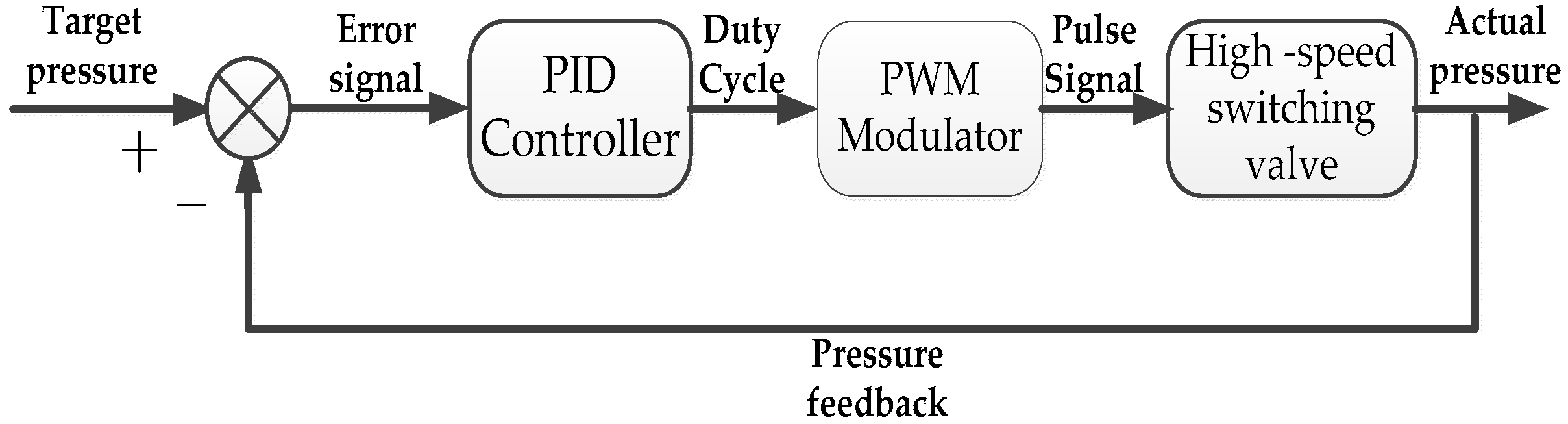
The pressure response characteristic of the braking system is an important factor to judge the performance of a braking system. A regenerative braking system requires a pressure braking system with good pressure control accuracy. In this study, a simple, effective, robust, reliable, and adaptable PID controller is adopted. The detailed control procedure is as follows: the wheel cylinder pressure sensor measures the actual pressure and thereafter inputs the error between the actual wheel pressure and target pressure to the PID controller, which calculates the duty cycle of the pulse width for controlling the high-speed switch valve, so that the wheel pressure can follow the target pressure. The control schematic is shown in Figure 9. The mathematical model of the controller is expressed in Equations (31) and (32):
where denotes the pulse-width modulation (PWM) duty cycle of the high-speed switch valve denotes the target pressure, denotes the actual pressure of the cylinder, and denotes the pressure difference.
3.5. Simulation Model of the Braking System
Considering the reflux pump model, hydraulic pipe model, and braking cylinder dynamic model, the physical model of the pressure coordinated control system is established in AMESim. Owing to the symmetry of the system, the half of the system structure is considered as the schematic, as shown in Figure 10.
3.6. Simulation and Analysis of Dynamic Characteristics of Braking System
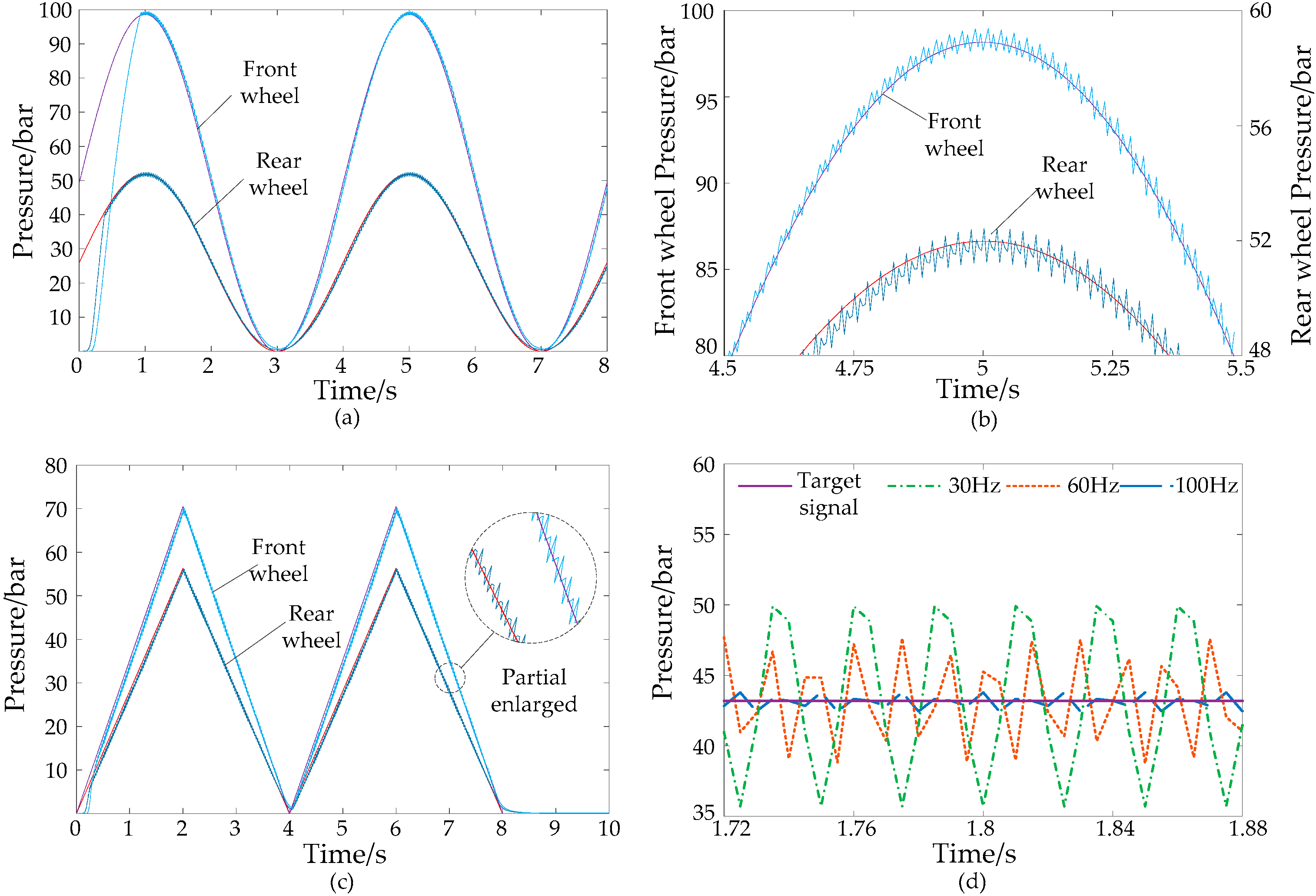
Inputting sine signals and sawtooth signals to the system, the pressure response curve of the system obtained is shown in Figure 11a–c.
It can be observed that, in the initial stage of braking, the hydraulic pressure is not built up within 0.1 s because the hydraulic oil must be filled into the braking clearance of the wheel cylinder and the expansion of the pipeline, and thereafter, the wheel cylinder pressure quickly reaches the target pressure. The time required to reach the wheel cylinder target pressure is related to the size of the target pressure. As shown in the locally enlarged figure, the braking pressure of the front and rear wheels is still pulsating in the steady state, the average value of the pressure at the front and rear wheel can coincide well with the target signal, and the system shows good performance in terms of pressure response and tracking.
Figure 11d shows the pressure response to the target signal under different PWM modulation frequencies. The results show that the modulation frequency of the high-speed switch valve has an important effect on the steady-state pressure fluctuations of the system. As the modulation frequency increases, the pressure fluctuation of the system becomes smaller.
4. Establishment of Simulation Model of Pressure Coordinated Control System Based on the Vehicle
4.1. Model of Control System
Using the system parameters mentioned above, the braking mode discrimination model, CVT controller model, braking force distribution controller model, and ABS controller model are established in Simulink, as shown in Figure 12.
Using Simulink and Stateflow to build the braking mode discrimination model, the input of the model is the braking intensity, vehicle speed, SOC and ABS trigger signal. The output is the mode switching valve control model, the return pump motor speed control signal, mode activation. Signals (pure hydraulic and regenerative braking), and clutch control signals.
The input of the braking force control model is the braking strength, the front and rear motor maximum braking torque, the vehicle speed, the CVT speed ratio and the braking mode activation signal, and then the output signal is the AMESim medium and front motor demand electric mechanism power signal and the high speed switching valve control signal.
The front motor can provide braking force as much as possible by adjusting the CVT ratio during regenerative braking. The motor target speed n can be obtained by calculating the required front motor braking power, and hence, the CVT target ratio is:
where denotes the front wheel radius, denotes the motor speed (r/min) denotes the ratio of the front final drive, and denotes the vehicle speed (km/h).
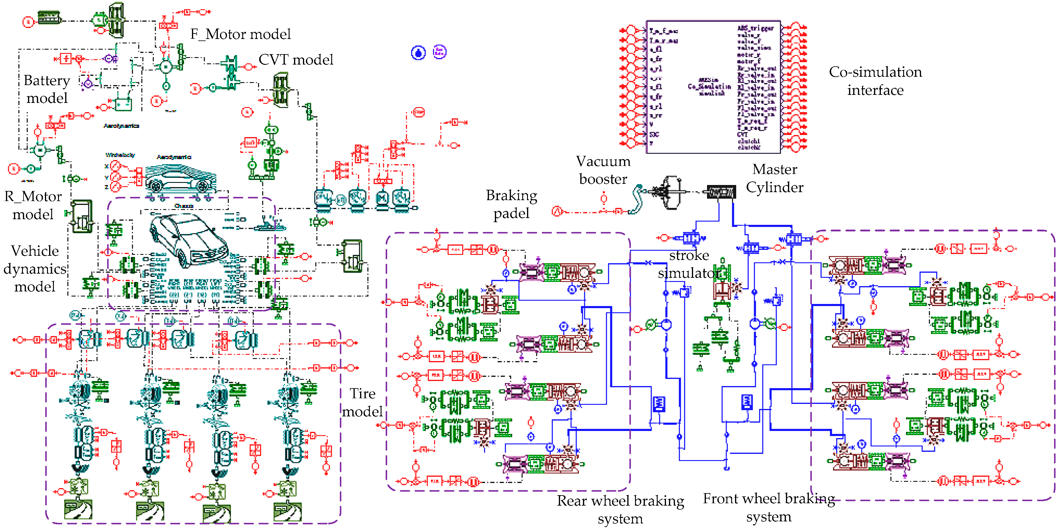
4.2. Establishment of Co-Simulation Model
The braking system hardware model, motor model, battery model, tire model, CVT model, and 15-degrees-of-freedom vehicle dynamics model are established in AMESim as shown in Figure 13.
5. Simulation and Analysis of Dynamic Characteristics of Braking System Based on the Vehicle
5.1. Simulation and Analysis under Variable Braking Strength
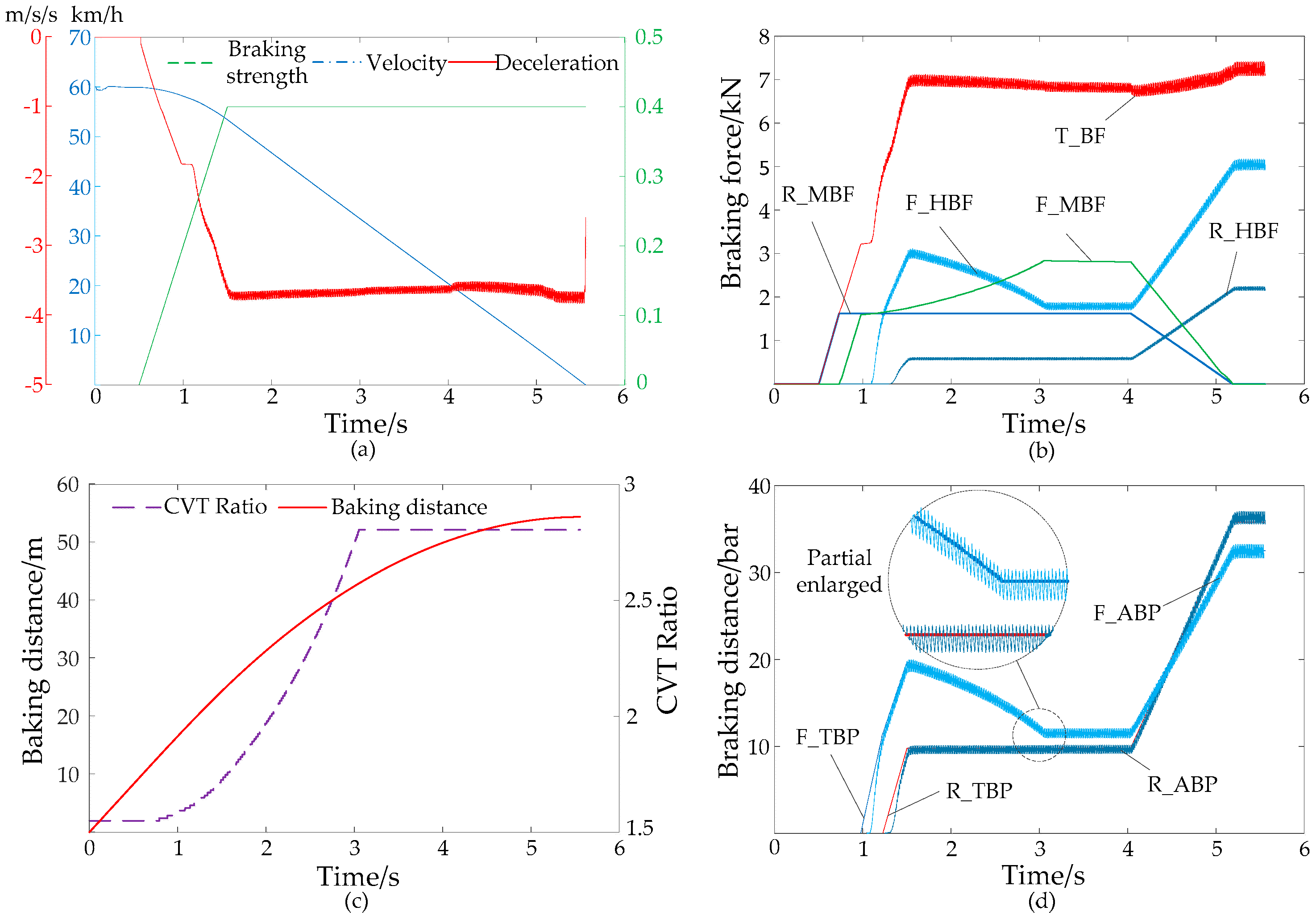
In the simulation of variable braking strength, the initial SOC is 0.7, the initial braking speed is 60 km/h, the initial CVT ratio is 1.55, and the braking strength increases by 0.1/s starting from 0.5 s. It can be observed from Figure 14b that, during the braking process, the braking force is first provided by the rear motor. As the braking strength increases, the braking force of the front motor is added to the braking when the rear motor cannot provide sufficient braking force. When the motor braking force reaches its maximum, the front axle hydraulic pressure is added to the braking in 2.7 s. During the initial stage of pressure built-up, the braking fluid should be filled into the clearance of the braking block and the braking pipe expansion, and hence, the total braking force is temporarily maintained. As the vehicle speed decreases and the CVT ratio is adjusted as shown in Figure 14c, the maximum braking force of the front motor increases and the hydraulic braking force of the front axle also increases to ensure the required braking force. At 3.6 s, the rear axle hydraulic braking force is also added. When the vehicle speed is less than 20 km/h, the front and rear motor braking forces gradually decrease. The decrease in vehicle speed leads to the decrease in motor speed, which further reduces the motor energy recovery capability. To ensure the total required braking force, the front and rear axle hydraulic braking forces should supplement the reduction of motor braking force. As shown in Figure 14a, as the braking strength increases, the braking deceleration follows the target deceleration well and the vehicle speed decreases smoothly. The braking distance is 74 m.
The pressure tracking performance of the front and rear wheel braking cylinders of the braking system is shown in Figure 14d. It can be observed that, owing to the operating characteristics of the front and rear motors, the required target braking pressure should satisfy linear and non-linear growth. The simulation results show that the cylinder actual pressure can follow the linear and non-linear target pressure precisely.
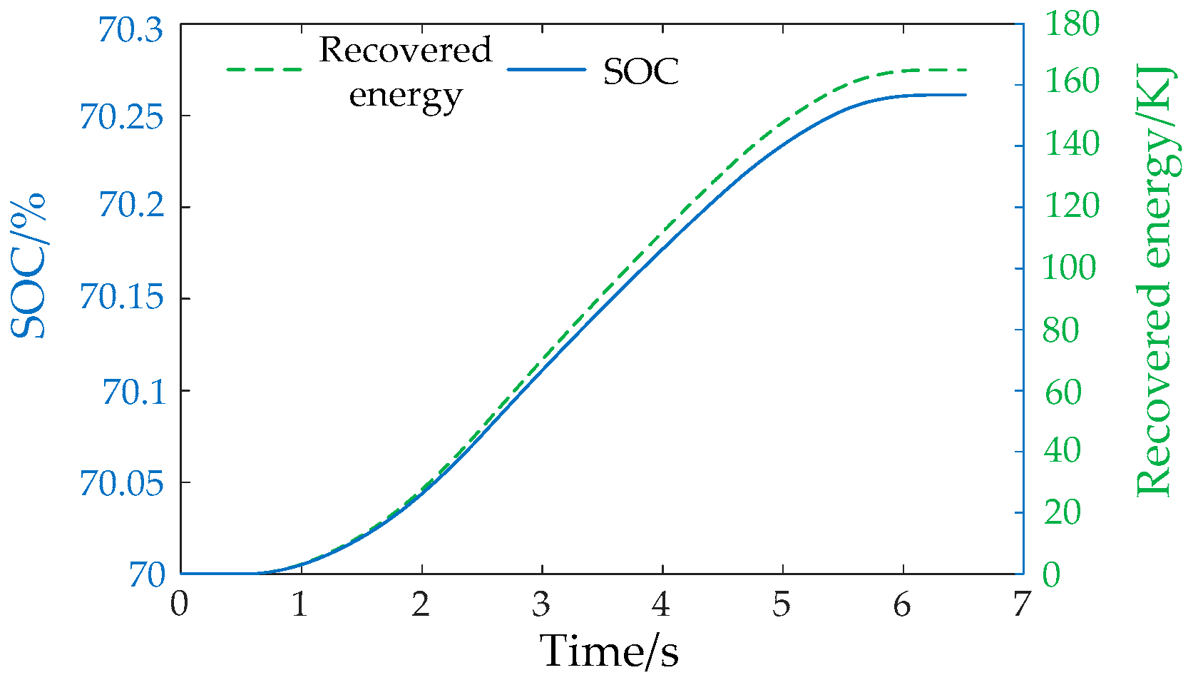
Energy recovery rate is an important criterion to judge the performance of a regenerative braking system. As shown in Figure 15, during the braking process, the SOC increases from 0.7 to 0.7026 and the battery’s state of charge recovery rate is 0.37%. The recovered energy is 165 kJ, which accounts for 66% of the total braking energy.
5.2. Simulation and Analysis under Constant Braking Strength
In the simulation under the condition of constant braking strength, the initial SOC is 0.7, the initial braking speed is 60 km/h, the CVT initial ratio is 1.5, and the braking strength starts increasing from 0.5 s. When the braking strength reaches 0.4 at 1.5 s, it remains constant. As shown in Figure 16a,b, the braking system responds well and the total braking force satisfies the requirements of the driver. In the braking process, the total braking force fluctuates slightly. This is because the change of CVT ratio during braking leads to a change in the efficiency of the CVT, and consequently, the braking force of the motor cannot follow the motor target braking force accurately. However, it can be observed from Figure 16a–c that the braking deceleration remains steady, the speed of the vehicle steadily decreases, and the braking distance is 54 m.
As shown in Figure 16d, the hydraulic braking force can follow the target braking force precisely and the mean value of actual braking pressure is coincident with the target braking pressure, which is shown in the local amplification area. Good dynamic and static characteristics of the hydraulic braking system are demonstrated.
As shown in Figure 17, during the braking process, the SOC increases from 0.7 to 0.7022 and the battery’s state of charge recovery rate is 0.31%. The energy recovered is 138 kJ, which accounts for 55% of the total braking energy.
5.3. Simulation and Analysis under Conventional Braking
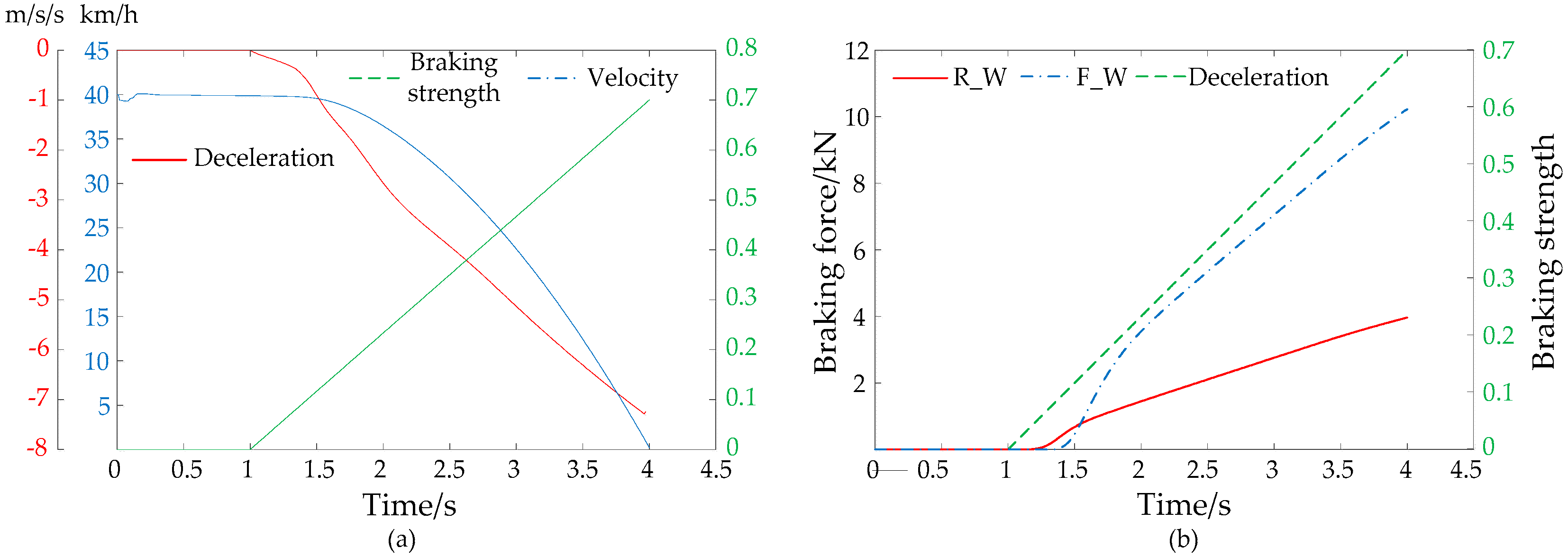
When in conventional braking mode, the braking master cylinder and wheel cylinder are connected, and the braking wheel cylinder pressure is provided by the master braking cylinder. As shown in Figure 18a, in the simulation under the condition of conventional braking, the initial braking speed is 40 km/h, and the braking strength increases by 0.23/s starting from 0.5 s. As shown in Figure 18b, owing to resistance along the way, the wheel cylinder clearance, and other factors, the response of braking force of the front and rear wheel lag behind the driver’s braking strength requirements. It can be observed from Figure 18a that the braking deceleration steadily increases, the speed of the vehicle steadily decreases, and the braking distance is 54 m. The result shows the system meets the braking demand of a hybrid vehicle in the conventional braking.
5.4. Simulation and Analysis of ABS
In this study, the wheel slip rate S and wheel acceleration and deceleration are used as the logic threshold for ABS control [16]. In the simulation, the road adhesion coefficient is 0.15, the initial speed of the vehicle is 70 km/h, and moderate-strength braking is carried out. As shown in Figure 19b, when the ABS is triggered, the front and rear motor braking forces gradually withdraw whereas the hydraulic braking force is added to the anti-lock brake. Each ABS control cycle includes pressurization, pressure hold, pressure reduce, and step boost pressurization. As shown in Figure 19d, the front and rear wheel slip ratios fluctuate around the target value of 0.2. At 14 s, the speed is reduced to 10 km/h; it is not suitable to use ABS anymore, the ABS exists, and the wheels are fully locked. During braking process, the vehicle deceleration fluctuates slightly, and the vehicle speed declines steadily. After the entire braking process, the braking distance is 166 m. Simulation results show that the system has good anti-lock performance.
5.5. Analysis and Simulation of Integrated Braking for the System
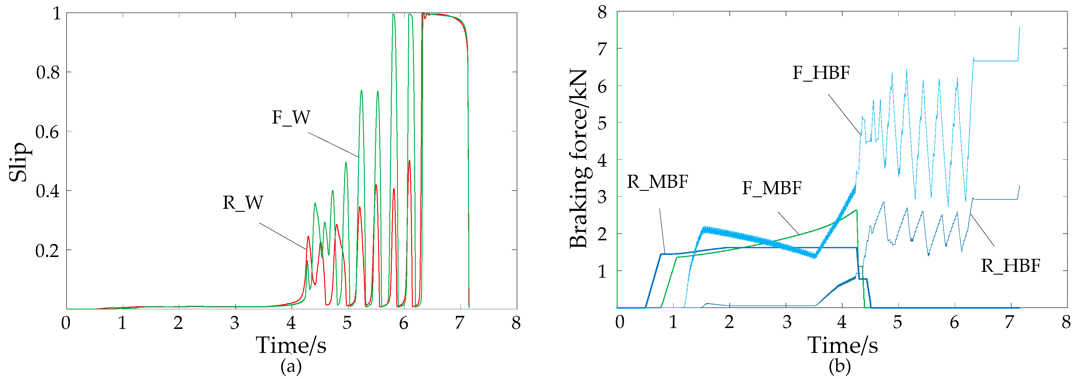
In the integrated braking simulation, the initial SOC is 0.7, the initial speed of the vehicle is 70 km/h, and the road adhesion coefficient is 0.4. The braking pedal inputs the braking strength signal as shown in Figure 20. The braking strength starts to increase from 0.5 s to 1.5 s, reaches 0.3, and remains constant until 3.5 s. Subsequently, the braking strength continues to increase until the braking strength reaches 0.8 at 5.5 s and thereafter remains constant until the vehicle stops. Figure 20 shows the variation of vehicle speed and wheel speed. Figure 21a shows the variation of slip rate. Figure 21b shows the variation of braking force.
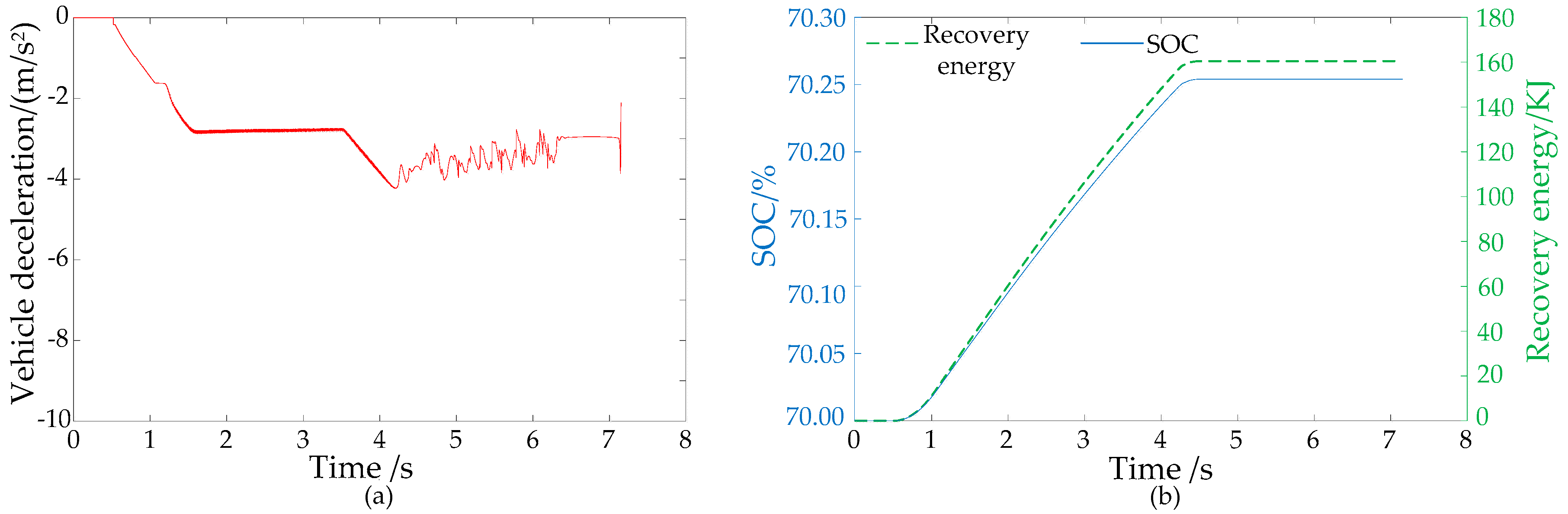
It can be observed from the simulation results that as the braking strength increases, the braking force of the motor and the hydraulic braking force are successively added to the braking. At 4.1 s, the wheels tend to be locked, and ABS is triggered. The front and rear motor braking forces gradually withdraw with the coordination of the hydraulic braking force. The pressure control system controls the wheel slip ratio fluctuating around the optimum value as shown in Figure 22a. At 6.2 s, the vehicle speed is less than 10 km/h, the ABS exists, and the wheels are fully locked. The variation of vehicle deceleration is shown in Figure 22a. As shown in Figure 22b, in the braking process, the SOC increases from 0.7 to 0.7025 and the battery’s state of charge recovery rate is 0.36%. The energy recovered is 160.5 kJ, which accounts for 46% of the total braking energy.
6. Conclusions
In this paper, according to the characteristics and required braking system functions of front and rear dual-motor-driven hybrid electric vehicles, a braking control strategy for an electro-hydraulic braking system with conventional braking and regenerative braking is proposed. The strategy ensures full utilization of motor braking force, which can improve the energy recovery rate in regenerative braking mode, and, under specific conditions, can assist as conventional braking.
A new type of pressure control system was designed based on the functional requirements of the brake system and based on the ABS hardware. The system fulfills the requirements of different operating modes for regenerative braking, conventional braking and ABS braking. At the same time, under the condition of regenerative braking, the coordinated control of the brake pressure in different working modes is realized through the ABS-based hardware pressure coordinated control.
Considering the required function of the braking system, the finite element analysis is used to establish electromagnet model, which makes the solenoid valve model more accurate. A simulation model of hydraulic braking system is established in AMESim and a PID controller is used to adjust the duty cycle of the pulse width signal, which is required by the high-speed switch valve to realize dynamic adjustment of wheel cylinder pressure. Simulation results show that the pressure coordinated control system has high response speed and accuracy, and it meets the braking demand of a hybrid vehicle.
Based on the designed brake system structure scheme, control scheme and mathematical model of hydraulic brake system, a vehicle-based AMESim-Simulink joint simulation platform is constructed. By simulating the system under variable-strength braking, constant-strength braking, conventional braking, ABS braking, and integrated braking, the system braking force control strategy and the dynamic performance of the braking pressure coordinated control system are verified. Results show that the braking energy recovery rate reaches 47~66% and the system has good static and dynamic characteristics and can quickly and accurately track the target braking pressure. Moreover, the ABS function can be realized well.
In summary, this system can realize the braking force distribution control strategy under different driving conditions by pressure coordinated control under the premise of meeting the braking demand, which improves the fuel economy of the vehicle and reduces emissions. If it is applied to a real vehicle, the structural parameters of the system can be further optimized to reduce the structural cost. If it is applied to a real vehicle, the structural parameters of the system can be further optimized to reduce the structural cost.
Author Contributions
Y.Y. designed the electric-hydraulic system and proposed the control strategies; G.L. conducted model building, calculation and analysis based on proposed control strategies; Q.Z. matched the parameters of the electric-hydraulic system and analyzed system performance.
Funding
The research is supported by: (1) the National Natural Science Foundation of China (51575063); (2) the Fundamental Research Funds for the Central Universities (No:106112016CDJXZ338825). The authors would also like to acknowledge the support from the State Key Laboratory of Mechanical Transmission of Chongqing University, China. The authors are indebted to the people who have helped to improve the paper.
Conflicts of Interest
The authors declare no conflict of interest.
References
- Khastgir, S.; Warule, P. Regenerative Braking Strategy for an Unaltered Mechanical Braking System of a Conventional Vehicle Converted into a Hybrid Vehicle. Available online: https://www.sae.org/publications/technical-papers/content/2013-26-0155/ (accessed on 16 August 2018).
- Lian, Y.F.; Tian, Y.T.; Hu, L.L.; Yin, C. A new braking force distribution strategy for electric vehicle based on regenerative braking strength continuity. J. Cent. South Univ. 2013, 20, 3481–3489. [Google Scholar] [CrossRef]
- Liang, Y.; Liang, C.; Zhou, F.; Liu, M.; Zhang, Y.; Wei, W. Simulation and analysis of potential of energy-saving from braking energy recovery of electric vehicle. J. Jilin Univ. 2013, 43, 6–11. [Google Scholar]
- Liu, Y.; Sun, Z.; Wang, M. Decoupled Electro-Hydraulic Brake System for New Energy Vehicles. Available online: http://dl5.tongji.edu.cn/handle/310200/12185 (accessed on 16 August 2018).
- Fujimoto, H.; Harada, S. Model-based range extension control system for electric vehicles with front and rear driving–braking force distributions. IEEE Trans. Ind. Electron. 2015, 62. [Google Scholar] [CrossRef]
- Hernández, M.I.G.; Pérez, B.A.; Sánchez, J.S.M.; Álvarez, E.C. Optimized regenerative friction braking distribution in an electric vehicle with four in-wheel motors. Adv. Microsyst. Automot. Appl. 2013, 2013. [Google Scholar] [CrossRef]
- Itani, K.; Bernardinis, A.D.; Khatir, Z.; Khatir, A. Comparison between two braking control methods integrating energy recovery for a two-wheel front driven electric vehicle. Energy Convers. Manag. 2016, 122, 330–343. [Google Scholar] [CrossRef]
- Nakamura, E.; Soga, M.; Sakai, A.; Otomo, A.; Kobayashi, T. Development of Electronically Controlled Braking System for Hybrid Vehicle. Available online: https://www.sae.org/publications/technical-papers/content/2002-01-0300/ (accessed on 16 August 2018).
- Ko, J.W.; Ko, S.Y.; Kim, I.S.; Hyun, D.Y.; Kim, H.S. Co-operative control for regenerative braking and friction braking to increase energy recovery without wheel lock. Int. J. Auto. Technol. 2014, 15, 253–262. [Google Scholar] [CrossRef]
- Peeie, M.H.B.; Ogino, H.; Oshinoya, Y. Skid control of a small electric vehicle with two in-wheel motors: Simulation model of ABS and regenerative brake control. Int. J. Crashworth. 2016, 21, 396–406. [Google Scholar] [CrossRef]
- Li, L.; Li, X.; Wang, X.; Liu, Y.; Song, J.; Ran, X. Transient switching control strategy from regenerative braking to anti-lock braking with a semi-brake-by-wire system. Veh. Syst. Dyn. 2016, 54, 231–257. [Google Scholar] [CrossRef]
- Cheon, J.S. Brake By Wire System Configuration and Functions using Front EWB (Electric Wedge Brake) and Rear EMB (Electro-Mechanical Brake) Actuators. Available online: https://www.sae.org/publications/technical-papers/content/2010-01-1708/ (accessed on 16 August 2018).
- Ko, J.; Ko, S.; Son, H.; Yoo, B.; Cheon, J.; Kim, H. Development of Brake System and Regenerative Braking Cooperative Control Algorithm for Automatic-Transmission-Based Hybrid Electric Vehicles. IEEE Trans. Veh. Technol. 2015, 64, 431–440. [Google Scholar] [CrossRef]
- Wang, M.; Sun, Z.; Zhuo, G.; Cheng, P. Maximum Braking Energy Recovery of Electric Vehicles and Its Influencing Factors. Available online: http://en.cnki.com.cn/Article_en/CJFDTOTAL-TJDZ201204016.htm (accessed on 16 August 2018).
- Tao, R.; Zhang, H.; Fu, D.; Xia, Q. Simulation of ABS hydraulic system and optimization of solenoid valve. Trans. CSAE 2010, 26, 135–139, (In Chinese with English Abstract). [Google Scholar]
- Du, Y.C.; Qin, C.A.; You, S.Y.; Xia, H.C. Efficient coordinated control of regenerative braking with pneumatic anti-lock braking for hybrid electric vehicle. Sci. China Technol. Sc. 2017, 60, 399–411. [Google Scholar] [CrossRef]
Figure 1.
Schematic diagram of a dual-motor driven HEV electro-hydraulic braking system. VCU: Vehicle Control Unit; MCU: Motor Controller Unit; HCU: Hybrid Control Unit; ECU: Engine Control Unit; BCU: Battery Control Unit; TCU: Transmission Control Unit.
Figure 1.
Schematic diagram of a dual-motor driven HEV electro-hydraulic braking system. VCU: Vehicle Control Unit; MCU: Motor Controller Unit; HCU: Hybrid Control Unit; ECU: Engine Control Unit; BCU: Battery Control Unit; TCU: Transmission Control Unit.
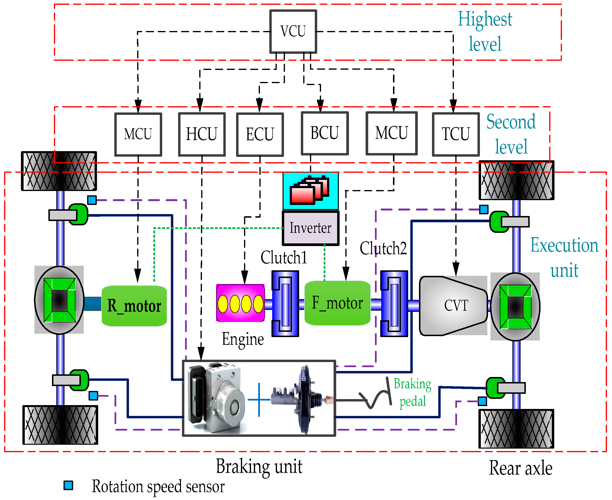
Figure 2.
Control flowchart of the pressure coordinated control system.
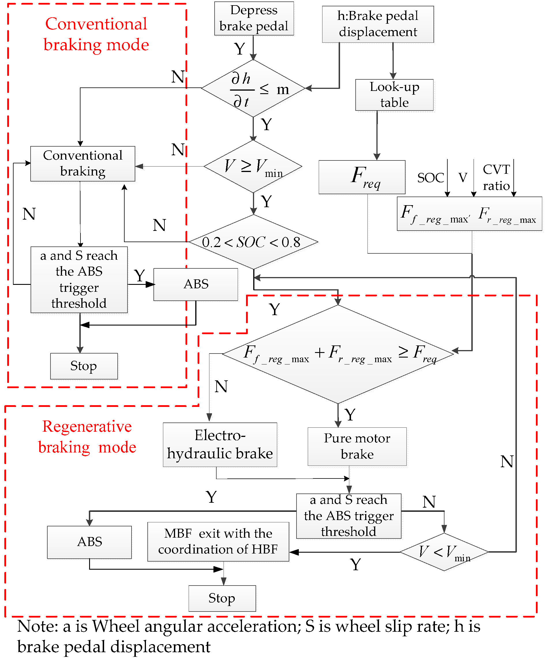
Figure 3.
Braking force distribution curve.

Figure 4.
Braking system pressure coordinated control diagram.

Figure 5.
Schematic diagram of the pressure coordinated control system.

Figure 6.
Structure diagram of high-speed switch reducing valve.

Figure 7.
Model of electromagnet: (a) Finite element analysis of electromagnet, (b) Diagram of electromagnetic force, current and displacement.
Figure 7.
Model of electromagnet: (a) Finite element analysis of electromagnet, (b) Diagram of electromagnetic force, current and displacement.

Figure 8.
AMESim model of normally closed valve.
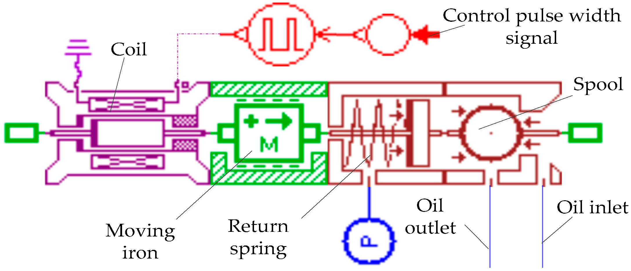
Figure 9.
PID control schematic of wheel cylinder pressure.

Figure 10.
AMESim model of wheel cylinder pressure control system.
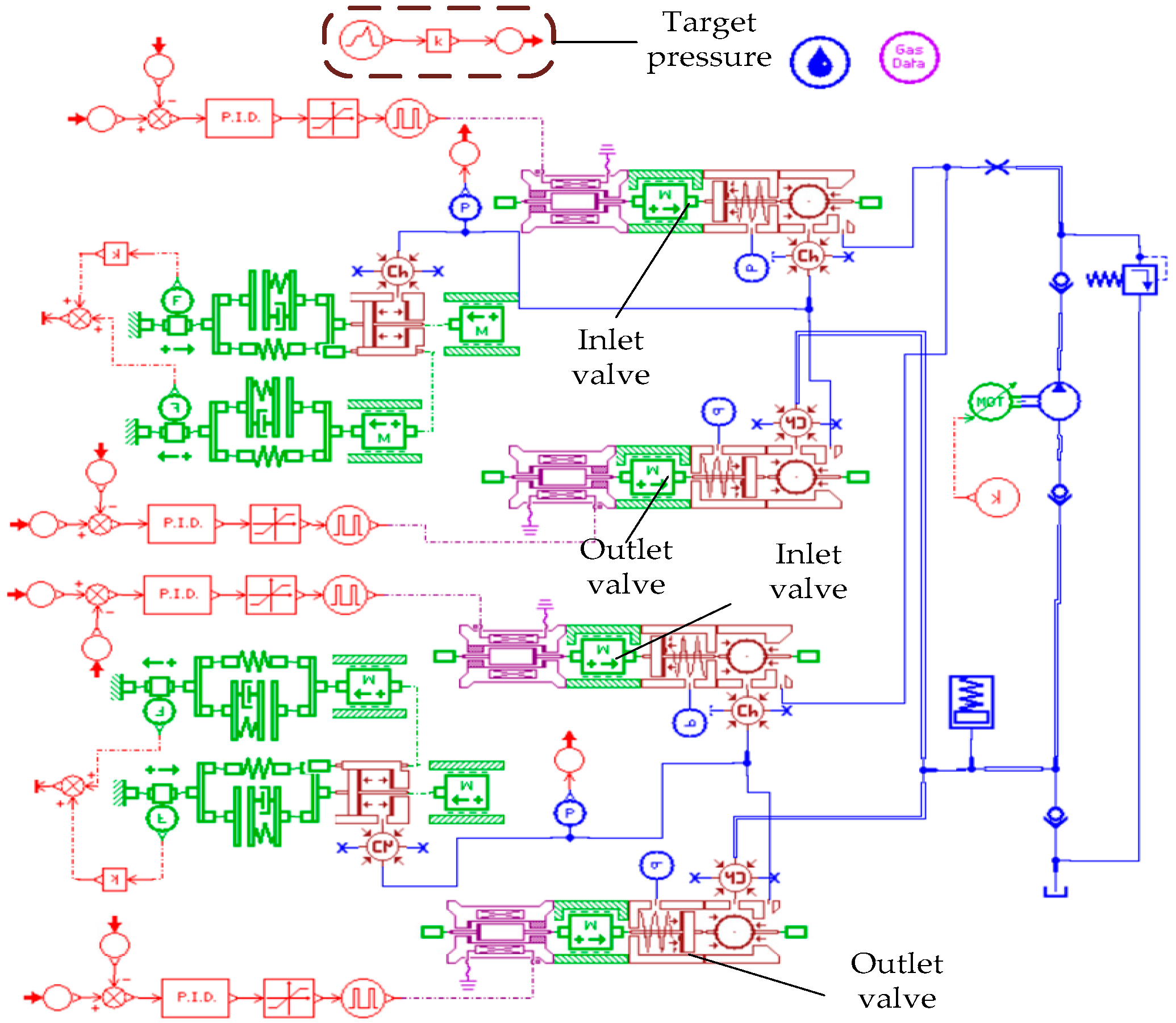
Figure 11.
The simulation of the braking system: (a) Response curves of the sinusoidal signal, (b) Partial enlarged diagram, (c) Response curves of a sawtooth signal, (d) Pressure fluctuations curves at different modulation frequencies.
Figure 11.
The simulation of the braking system: (a) Response curves of the sinusoidal signal, (b) Partial enlarged diagram, (c) Response curves of a sawtooth signal, (d) Pressure fluctuations curves at different modulation frequencies.

Figure 12.
Simulink model of control system.
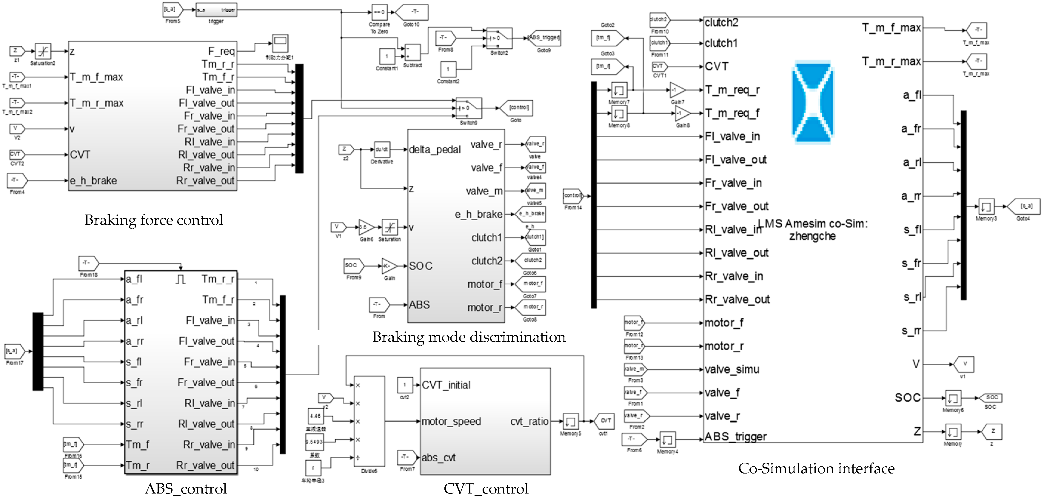
Figure 13.
AMESim model of pressure coordinated system and vehicle system.

Figure 14.
Simulation under variable braking strength: (a) Variation of braking strength, vehicle speed and deceleration, (b) Variation of braking force, (c) Variation of CVT ratio and braking distance, (d) Pressure response curve of braking system.
Figure 14.
Simulation under variable braking strength: (a) Variation of braking strength, vehicle speed and deceleration, (b) Variation of braking force, (c) Variation of CVT ratio and braking distance, (d) Pressure response curve of braking system.

Figure 15.
Variation of recovery energy and SOC under variable braking strength.

Figure 16.
Simulation under constant braking strength: (a) Variation of braking strength, vehicle speed, and deceleration, (b) Variation of braking force, (c) Variation of CVT ratio and braking distance, (d) Pressure response curve of braking system.
Figure 16.
Simulation under constant braking strength: (a) Variation of braking strength, vehicle speed, and deceleration, (b) Variation of braking force, (c) Variation of CVT ratio and braking distance, (d) Pressure response curve of braking system.

Figure 17.
Variation of recovery energy and SOC under constant braking strength.
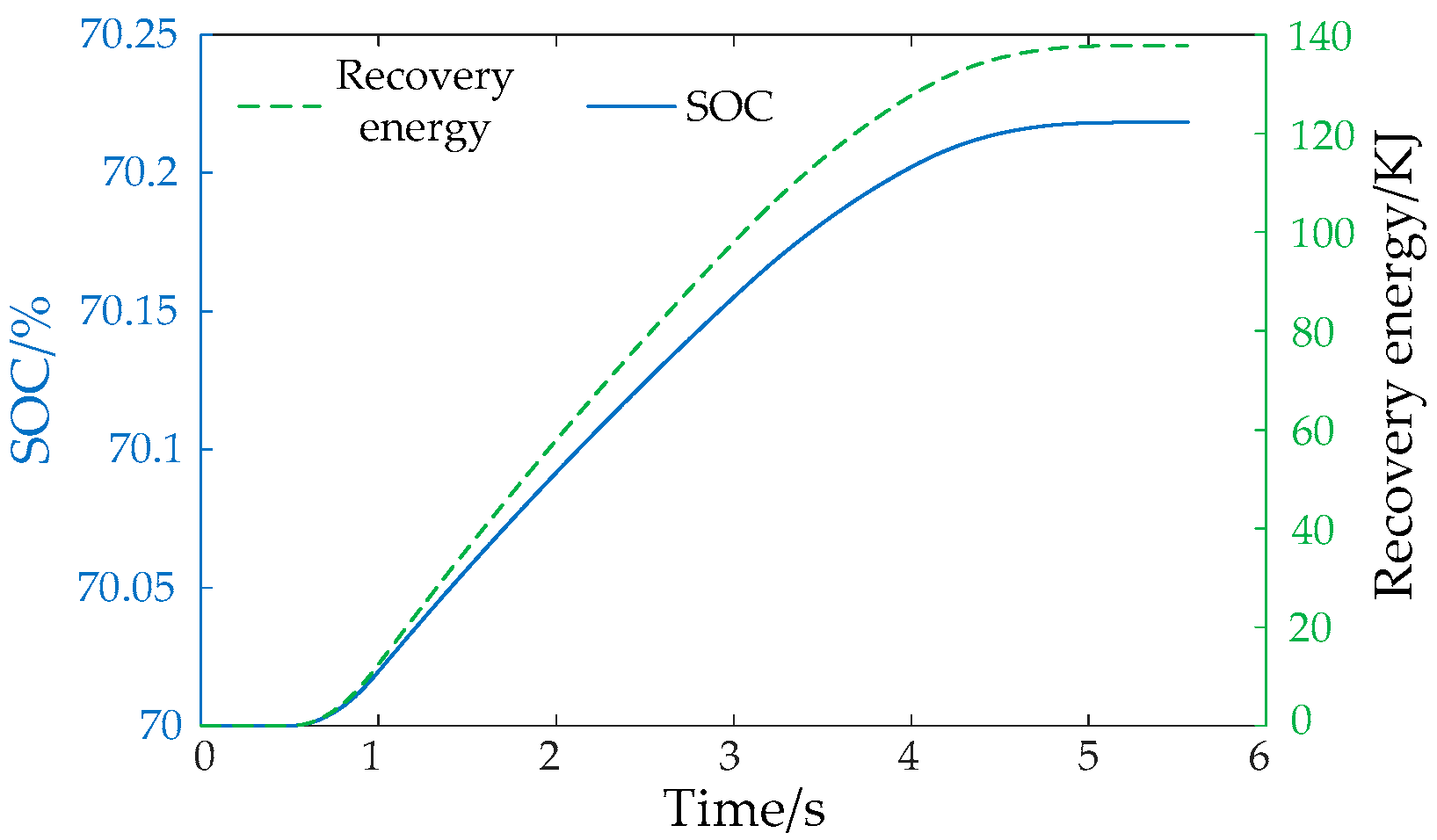
Figure 18.
Simulation under conventional braking: (a) Variation of braking strength, vehicle speed and deceleration, (b) Variation of front/rear wheel braking force and braking strength.
Figure 18.
Simulation under conventional braking: (a) Variation of braking strength, vehicle speed and deceleration, (b) Variation of front/rear wheel braking force and braking strength.

Figure 19.
Simulation of ABS: (a) Variation of braking strength, vehicle speed and wheel speed, (b) Variation of braking force, (c) Variation of wheel angle acceleration, (d) Variation of front and rear wheel slip rate, (e) Variation of vehicle deceleration and braking distance.
Figure 19.
Simulation of ABS: (a) Variation of braking strength, vehicle speed and wheel speed, (b) Variation of braking force, (c) Variation of wheel angle acceleration, (d) Variation of front and rear wheel slip rate, (e) Variation of vehicle deceleration and braking distance.
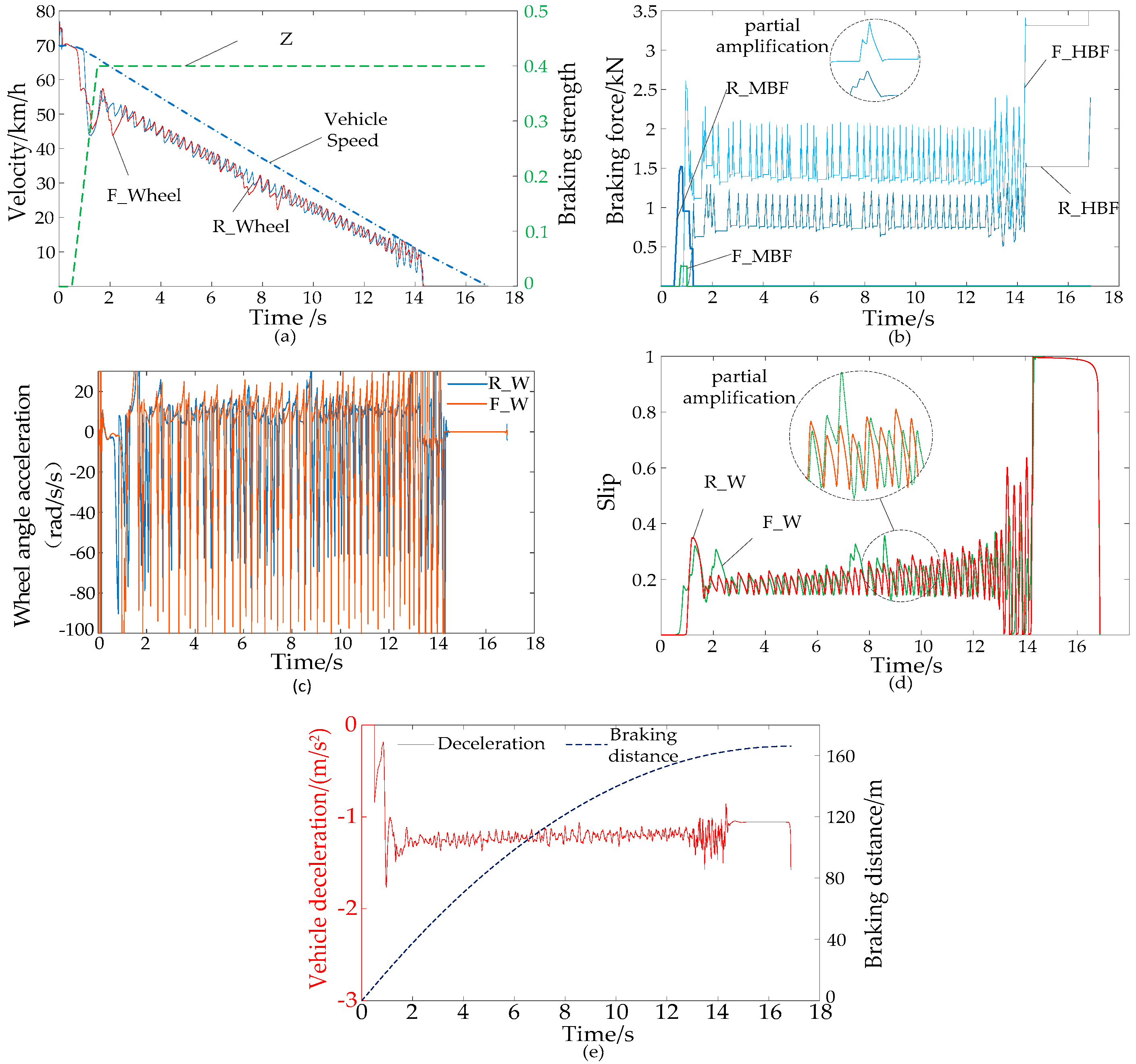
Figure 20.
Variation of braking strength, vehicle speed and wheel speed under integrated braking.

Figure 21.
Simulation under integrated braking: (a) Variation of front and rear wheel slip rate, (b) Variation of braking force under integrated braking.
Figure 21.
Simulation under integrated braking: (a) Variation of front and rear wheel slip rate, (b) Variation of braking force under integrated braking.

Figure 22.
Simulation under integrated braking: (a) Variation of braking deceleration, (b) Variation of SOC and recovery energy.
Figure 22.
Simulation under integrated braking: (a) Variation of braking deceleration, (b) Variation of SOC and recovery energy.

Table 1.
Main parameters of the vehicle.
| Parameter (Units) | Value |
|---|---|
| Vehicle mass (kg) | 1800 |
| Rolling radius (m) | 0.36 |
| Front motor rated/peak power (kW) | 14/28 |
| Rear motor rated/peak power (kW) | 13.5/27 |
| Battery capacity (Ah) | 38.43 |
Table 2.
Main parameters of the pressure coordinated control system.
| Parameter (Units) | Value |
|---|---|
| Front/rear braking cylinder diameter (mm) | 38.34/60.12 |
| Front/rear braking disc radius (mm) | 120/128 |
| Master cylinder diameter (mm) | 22.2 |
| Regulating valve pressure (MPa) | 11 |
| Modulation frequency of high-speed switch valve (Hz) | 90 |
| Pump displacement (mL/r) | 1 |
| Pump-motor rotating speed (r/min) | 2500 |
Table 3.
Main parameters of the high-speed switch valve.
| Parameter | Value |
|---|---|
| Return spring stiffness | 1.6 N/mm |
| Moving iron mass | 15 g |
| Coil turns | 380 |
| Coil resistance | 5 Ω |
| Initial air gap | 0.3 mm |
| Spool displacement | 0.22 mm |
| Voltage | 12 V |
| Spring preload force | 7 N |
© 2018 by the authors. Licensee MDPI, Basel, Switzerland. This article is an open access article distributed under the terms and conditions of the Creative Commons Attribution (CC BY) license (http://creativecommons.org/licenses/by/4.0/).
Share and Cite
MDPI and ACS Style
Yang, Y.; Li, G.; Zhang, Q. A Pressure-Coordinated Control for Vehicle Electro-Hydraulic Braking Systems. Energies 2018, 11, 2336. https://doi.org/10.3390/en11092336
AMA Style
Yang Y, Li G, Zhang Q. A Pressure-Coordinated Control for Vehicle Electro-Hydraulic Braking Systems. Energies. 2018; 11(9):2336. https://doi.org/10.3390/en11092336
Chicago/Turabian StyleYang, Yang, Guangzheng Li, and Quanrang Zhang. 2018. "A Pressure-Coordinated Control for Vehicle Electro-Hydraulic Braking Systems" Energies 11, no. 9: 2336. https://doi.org/10.3390/en11092336
Note that from the first issue of 2016, this journal uses article numbers instead of page numbers. See further details here.