Article

Constructing Accurate Equivalent Electrical Circuit Models of Lithium Iron Phosphate and Lead–Acid Battery Cells for Solar Home System Applications

1
Department of Electrical Sustainable Energy, Delft University of Technology, 2600 AA Delft, The Netherlands
2
Department of Radiation Science and Technology, Delft University of Technology, 2600 AA Delft, The Netherlands
*
Authors to whom correspondence should be addressed.
Energies 2018, 11(9), 2305; https://doi.org/10.3390/en11092305
Submission received: 7 August 2018 / Revised: 20 August 2018 / Accepted: 22 August 2018 / Published: 1 September 2018
(This article belongs to the Special Issue Battery Storage Technology for a Sustainable Future)

Abstract

:
The past few years have seen strong growth of solar-based off-grid energy solutions such as Solar Home Systems (SHS) as a means to ameliorate the grave problem of energy poverty. Battery storage is an essential component of SHS. An accurate battery model can play a vital role in SHS design. Knowing the dynamic behaviour of the battery is important for the battery sizing and estimating the battery behaviour for the chosen application at the system design stage. In this paper, an accurate cell level dynamic battery model based on the electrical equivalent circuit is constructed for two battery technologies: the valve regulated lead–acid (VRLA) battery and the LiFePO 4 (LFP) battery. Series of experiments were performed to obtain the relevant model parameters. This model is built for low C-rate applications (lower than 0.5 C-rate) as expected in SHS. The model considers the non-linear relation between the state of charge ( S O C ) and open circuit voltage ( V OC ) for both technologies. Additionally, the equivalent electrical circuit model for the VRLA battery was improved by including a 2nd order RC pair. The simulated model differs from the experimentally obtained result by less than 2%. This cell level battery model can be potentially scaled to battery pack level with flexible capacity, making the dynamic battery model a useful tool in SHS design.

1. Introduction

As of 2016, almost 1.1 billion people around the world lacked access to electricity [1]. While grid-extension is not always the most plausible solution, solar-based off-grid solutions such as solar home systems (SHS) have become prominent in use. Battery storage is an essential component of an SHS, as it is not only the most expensive component, but also the component with usually the least lifetime [2]. Therefore, understanding battery behaviour is critical for designing and analysing SHS.
In this study, two battery technologies commonly used in SHS were explored: the valve regulated lead–acid (VRLA) battery and the LiFePO 4 (LFP) battery. Lead–acid is the cheapest technology in the market in comparison with the other common battery technologies [3]. In particular, the valve regulated type of lead–acid battery is sealed, which reduces the risk of liquid leaking when compared to flooded lead–acid battery. Moreover, VRLA battery is entirely maintenance free [4]. In the case of LFP battery, it has surged as a predominant technology due to its appropriate chemical and thermal stability together with its high energy capacity [5]. Additionally, LFP batteries have experienced a reduction in price that is expected to continue [6].

1.1. Selecting the Battery Model

Depending on the application, accuracy, complexity, compatibility and universality, there are several technical methods to approach an expected battery model. Generally, there are three levels of battery models according to the degree of physical insight, viz., white box (e.g., electrochemical/physical model), grey box (e.g., equivalent electrical circuit model) and black box (e.g., artificial neural network model) [7].
The equivalent electrical circuit model (EECM) presents an equilibrium among computational time, precision, and complexity. As the EECM models the battery with only electrical components, this kind of models is highly compatible with other electrical models, which make them easy to implement with battery management systems and in other electrical engineering applications. Moreover, the construction of EECM does not have a very comprehensive co-relation with electrochemical processes inside the battery. As a result, there is no limitation on distinct battery types when modelling the battery by EECMs. Hence, the electrical equivalent circuit model (EECM) is selected in study.

1.2. Importance of Low Current Battery Models for SHS

Battery modelling is essential in SHS design, as they help to elucidate the relationship between power required by a predefined load and the operational conditions in which the batteries are used. Particularly, in SHS, the C-rates (related to the rate at which a battery is charged or discharged) are usually lower than 0.5 C, with the lowest C-rate being 1/120 C to 1/100 C [8,9].However, the existing battery cell level models do not focus on low C-rates; instead, they normally study a wide range of C-rates with high sampling resolution. For example, C-rates of 0.1 C, 0.5 C, 1 C, 2 C, 3 C, 4 C, 7 C, and 9 C have been proposed in [10], while other authors have explored C-rates of 0.04 C, 0.1 C, 1 C, 2 C, 3 C, 5 C, and 10 C [11], and 0.1 C, 0.5 C, 1 C, 2 C, 3 C, and 4 C [12]. Therefore, the applicability of these models in wide C-rate ranges does not necessarily validate their suitability for SHS.
Consequently, we focus on the low battery C-rates reflecting typical SHS applications. To obtain an accurate battery model which suitable for low C-rate applications, experiments with narrower C-rate range but with high sample resolutions are proposed. The applicable C-rate range of this model is 0.05 C–0.5 C with the sample resolution of 0.05 C–0.1 C.

1.3. Contributions

This papers contributes to the current state of the art by
  • developing an accurate battery cell level model especial for a low currents, as the case in SHS;
  • proposing a common modelling methodology based on electrical circuit model applicable to both VRLA and LFP batteries; and
  • improving the current electrical circuit models for VRLA battery including
     
    a non-linear relation between V OC and S O C ;
     
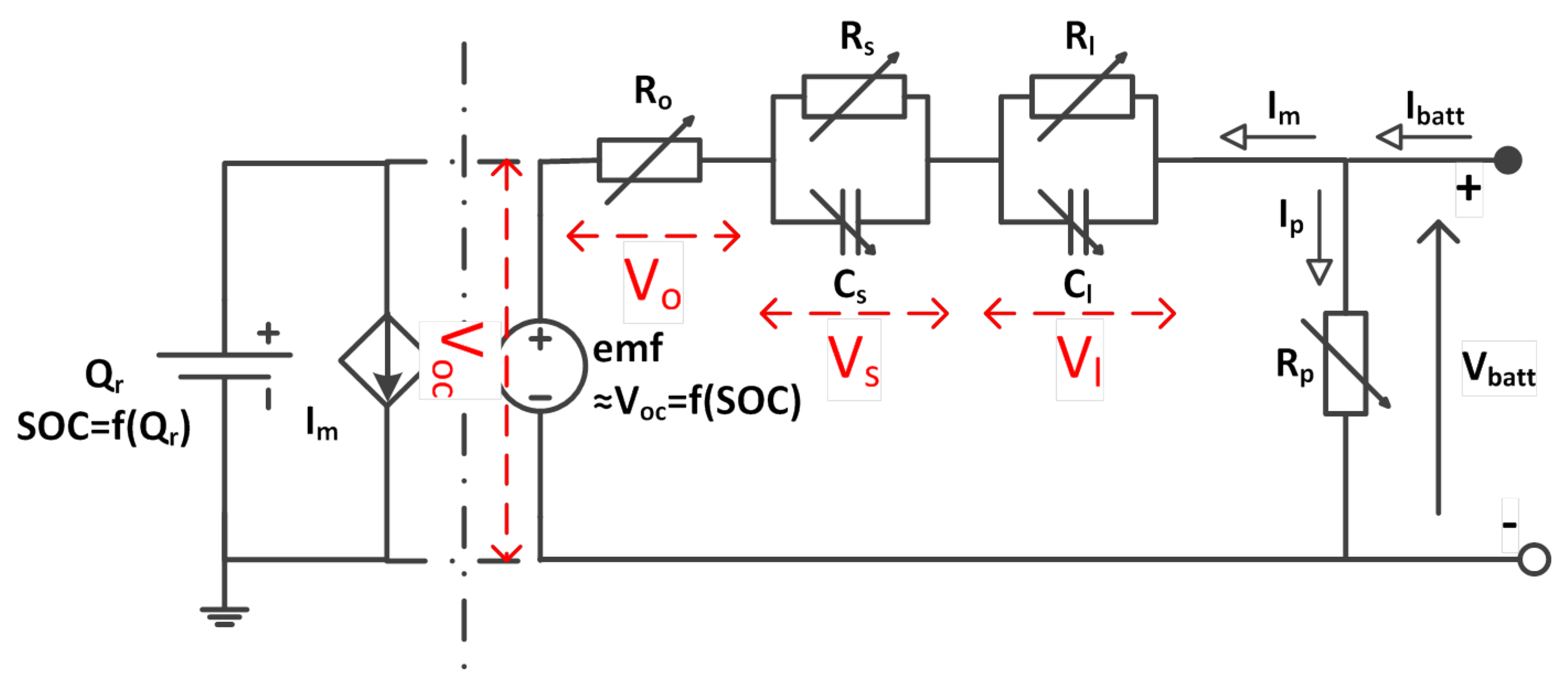
    a 2nd order RC circuit-based EECM model using a Thevenin approach;
     
    considering the parasitic branch of the EECM in terms of S O C and C-rate-based Coulombic efficiency.

2. Background

2.1. Battery Parameters

State of the Charge ( S O C ): S O C is usually defined as the proportion of the maximum possible electric charge that is present inside a rechargeable battery [13]. It is calculated by the ratio between the difference of the battery capacity and the net electric charge discharged from a battery since the last full state of charge. The S O C can be expressed by Equation (1).
S O C = Q t Q e Q t = Q r Q t
Q e = 0 t I m d τ
I m = I batt I p
where Q t is the temperature dependent actual capacity, Q e is the capacity that be extracted from the battery starting from its full state, and Q r is the capacity that remaining in the battery. I m is the main branch current, which is the result of the load current applied to the battery minus the current consumed in side-reactions ( I p ). I m is positive if the battery is discharging and I m is negative if the battery is charging.
Electromotive force (emf): The electromotive force of a cell is the algebraic sum of the potential difference of two half cells, which is the chemical potential of redox reactions happening on these two electrodes [14].
Open circuit voltage (OCV, or V OC ) and cte-OCV: The open circuit voltage (OCV) is the potential difference across its terminals when there is no current flow in or out of a reversible cell [15]. If the battery rests enough time (depending on the battery technology) with no current flow, the OCV can be called Close-to-Equilibrium open circuit voltage (cte-OCV) [16]. This value can be regarded as the estimated emf value.
Current rate (C-rate): The current rate, which is also called C-rate, is defined as the magnitude of charge/discharge current in Ampere to the nominal capacity of the battery in Ampere-hour. The C-rate represents the speed of charge/discharge, and it can be calculated using Equation (4) [17].
C r a t e = I batt Q n
where I batt is the current applied on the battery in the unit of ampere (A), and Q n is the nominal battery capacity in the unit of ampere hour (Ah).

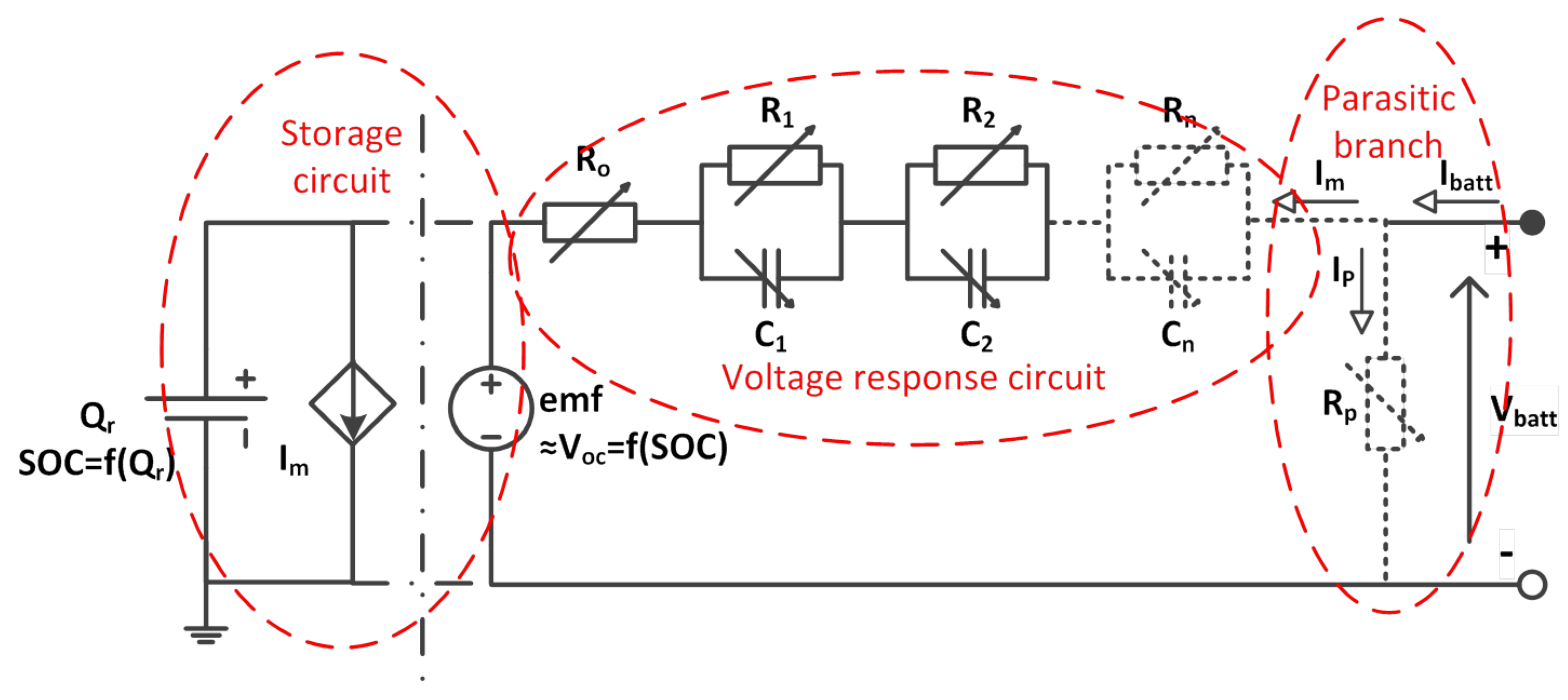
2.2. Construction of the Dynamic Battery Model

A good battery model should be capable of predicting both the battery storage capability information and the voltage response to the load. An equivalent electrical circuit model (EECM) can describe both characteristics. In some cases, modelling the side reactions is required in terms of battery losses, which is also possible to be realized with the EECM.
As shown in Figure 1, there are three main parts in the EECM to model the different features of the battery. First part is the storage circuit. Three parameters should be modelled in this sub-circuit: the battery capacity (which is the charge storage ability), the amount of charge is left in the battery ( S O C ), and the open circuit voltage V OC .
The second part is the voltage response circuit, which focuses on the internal structure of the battery. This makes it possible to imitate the electrical response of the battery under different loads. In this paper, a Thevenin model is applied, and it consists of a resistance in series with RC pairs.
The last part is the parasitic branch, which is used to model the side reactions that induce loss of charge in the battery. There are many ways to model these battery losses. For example, Figure 1 shows the parasitic branch in the form of a resistance ( R p ). For both battery technologies, the basic construction of EECM is applicable, as shown in Figure 1.

2.3. Storage Circuit

As discussed in Section 2.1, the cte-OCV can be regarded as the emf value. As the emf values are S O C dependent, the cte-OCV can be used as a S O C indicator. In this study, the S O C value is selected as the independent variable, while the coulomb counting method is used to determine the S O C . The S O C can be expressed by Equation (1).

2.4. Electrical Response Circuit

There is a deviation of voltage from the equilibrium state, also called polarization, whenever the battery is loaded. Conversely, the voltage recovers back towards the equilibrium state whenever the load is disconnected. Hence, a voltage relaxation phenomenon is observable in a no-load interval (also called rest interval) when the battery is operating. The battery internal impedance can be potentially extracted from this voltage relaxation.
The non-load rest interval during a discharge stage is shown in Figure 2b. The voltage response can be divided into two parts, viz., an instantaneous voltage jump right after the load is paused, followed by a gradual increase of the voltage towards the cte-OCV. Those two voltage responses are correlated with two electrical parts: the ohmic resistance R o , and the resistance/capacitance pairs ( R 1 C 1 , R 2 C 2 ), as introduced in the construction of EECM model in Figure 1.
Generally, there is an expected time window for each of the voltage response. An EECM containing two RC-pairs is assumed. It is suggested that, within a five seconds time-window, the voltage boost ( V o ) right after the load disconnection is induced by the ohmic resistance R o [18]. The time window for the rest of the gradual voltage increase caused by the RC pairs is called the time constant. The time constant reflects the rate of change of voltage; if the voltage changes faster, the time constant is smaller [19]. The increase in voltage right after the immediate voltage increase is the “short-term voltage response”. This short time interval ( τ 1 ) is expected to be around 10 seconds, and this voltage increase ( V 1 ) is related to the first RC-pair, which is the R 1 , C 1 in Figure 2b [20]. The following increase in voltage ( V 2 ) is then treated as the long-term voltage response after a long time interval ( τ 2 ), which corresponds to the second RC-pair ( R 2 , C 2 ), as shown in Figure 2b. It is possible to increase the number of RC-pairs and divide the voltage relaxation into more parts, with which the accuracy of the model is improved, such as the R n , C n in Figure 2b. Many authors suggest to model the lead–acid battery with first order RC circuit. However, for Li-ion batteries, all three orders of RC circuit model are commonly seen [12,21,22,23,24]. Eventually, the relaxation voltage will reach cte-OCV if the rest interval is long enough. However, it is necessary to strive an optimum balance between accuracy and complexity. Therefore, the study described in this paper has considered two RC pairs.
Curve fitting method was applied on each of the voltage relaxation results. The recognition of each part of the voltage and the corresponding time constant was done by nonlinear least squares curve fit in Matlab [20]. The distinct voltage and time constant values were then fitted into the RC circuit complete response equations to obtain the values of electrical elements in the model. The equations are listed below as Equations (5)–(9).
V interval = V 1 ( 1 e t τ 1 ) + V 2 ( 1 e t τ 2 ) + V o
V OC = V initial + V o + V 1 t + V 2 t
R o = V o I
R k = V k I
C k = τ k R k
where k = 1, 2, 3, ..., n.

2.5. Parasitic Reaction Circuit

The electrical components interpreted in the previous subsections describe the behaviour of the battery based on its main reactions. During operation, not all the battery energy is involved in its main (charging/discharging) reactions; there are unwanted side reactions responsible for loss of useful energy. Therefore, additional elements are needed to model a parasitic branch considering the side reactions.
Especially when charging a lead–acid battery, significant losses can occur, which has a huge impact on the battery dynamic behaviour. This is particularly true when the battery is at a high S O C (>95%). Therefore, the charge loss of VRLA during the charging stage is considered as the most dominant loss mechanism. This loss is mainly due to gassing and oxygen recombination, but the transient gassing phenomenon can be quite complex and unpredictable especially for VRLA batteries [25].
There are different methods to model the parasitic branch. Some models use a self-discharge conductance to represent the side reactions, where the conductance is the function of battery voltage, or side reaction related voltage and the temperature [21,22]. Some other models represent the side reaction by means of gassing current, as the function of water decomposition voltage and the temperature, instead of modelling the side branch circuit [26].
In this study, an equation is derived from the one proposed in [27]. This method is based on the principle that the losses incurred in the parasitic branch can be viewed as the Coulombic inefficiency of the battery. Therefore, this method models the parasitic branch in the form of the Coulombic efficiency as a function of S O C and the battery current, as shown in Equation (10).
η c = 1 e x p b a × I test I ref + c × ( S O C 1 )
where I ref is the reference current, and I test is the test current. a, b, and c are the experimentally derived empirical constants. It must be noted that, as the current terms in Equation (10) occur in the form of a ratio, the Coulombic efficiency can be considered as a function of C-rate as well.

3. Methods and Experiment

3.1. Choice of Operational Variables

For both battery technologies, each of the internal impedances is known to be, to some extent, influenced by the S O C , the temperature, and the current [28]. To obtain a proper dynamic battery model, a battery should ideally be tested with all three variables. However, the influence of operating temperature was not investigated in this study. All experiments were performed in a laboratory with the temperature controlled in the range of 20–22 C. Therefore, all experiments can be considered as under constant room temperature conditions. S O C and current (in the form of C-rate) were the main operational variables considered in this study.

3.2. Overall Methodology

The EECM model is assumed as shown in Figure 1, with two RC pairs. The choice of two RC pairs is justified in Section 4. For the task of fully constructing the EECM model for both VRLA and LFP batteries, the following methodology was followed involving experiments, data analysis, and model verification.
  • Experimentation. Series of experiments were performed to extract the parameters of each electrical element pertaining to every sub-circuit.
    (a)
    Storage circuit. The cte-OCV measurement method was performed.
    (b)
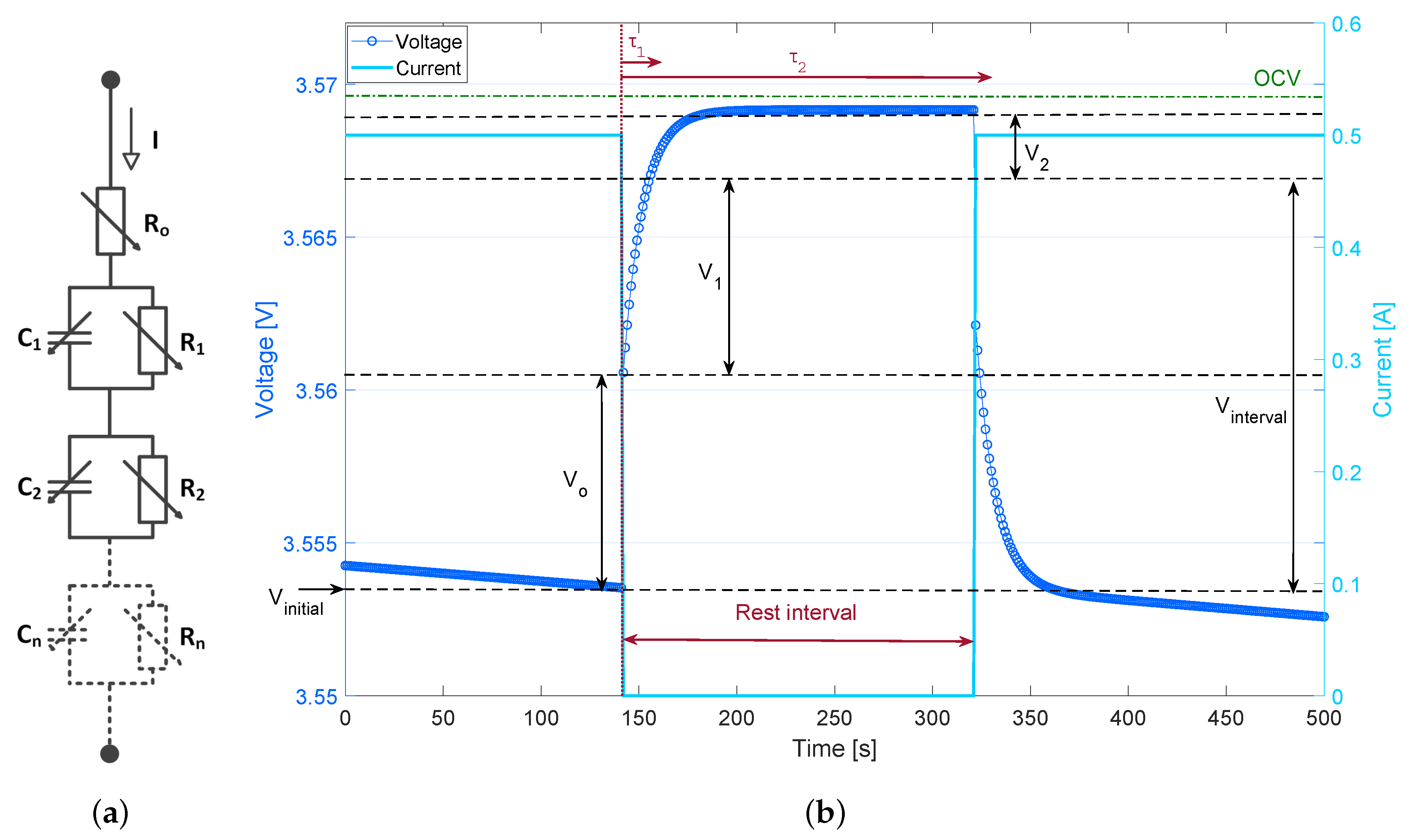
    Voltage response circuit. Voltage relaxation (also called step response) method was used.
    (c)
    Parasitic branch. The differential recharge efficiency measurement method was used.
    These measurements were applied on each featured S O C and with selected current rate, as further described in Table 1.
  • Parameter extraction. The parameters of each component in the EEMC were extracted and analyzed based on the experiments. The values of those parameters were then summarized into equations, and those equations can represent each of the electrical element in the electrical circuit.
  • EECM construction and model verification. All parts of the electrical elements were put together to construct the full EECM. Finally, the constructed EECM of each battery was simulated and compared with the experimental results.

3.3. Equipment and Materials

In this study, the battery tester used is MACCOR® Series 4000 Automated Test System [29]. The batteries selected for tests are Cyclon® AGM D single cell and A123systems® ANR26650M1B, and both of the battery cells have 2.5 Ah capacity [30,31].
The basic charge and discharge methods applied in this study are constant current (CC) method and constant current–constant voltage (CC-CV) method. The CC method involves charging or discharging the battery with a constant current until the battery voltage reaches a specific value. The specified voltage to stop the discharging process is called the end of discharge voltage (EODV). The CC-CV method involves first charging/discharging the battery with constant current until the battery voltage reaches the pre-set value, and then switch to constant voltage stage, which involves charging/discharging the battery with a constant voltage.
The in-detailed charge and discharge method of each battery technology is summarized in Table 1. This follows the recommendations and best practices outlined in the data sheets and previous articles [20,30,31,32].

3.4. Storage Circuit

The purpose of this set of experiments is to obtain the relation between the cte-OCV and the S O C . Therefore, the cte-OCV should be measured at different S O C values, and the battery is fully discharged before the measurement. During the experiments, the battery was monotonically charged to full and then discharged to empty, with both procedures being executed in steps of 5% S O C . Coulomb-counting method was used to approach the designated S O C demarcation. After each step, the battery was rested for a constant time to reach the close-to-equilibrium state, at which point the voltage was measured and noted as the cte-OCV value. The C-rate was 0.2, while the rest time was 3 h for VRLA battery and 4 h for LFP battery. Three battery cells were tested to get a result with better accuracy.
The experimental procedure is illustrated in the flowchart shown in Figure 3.

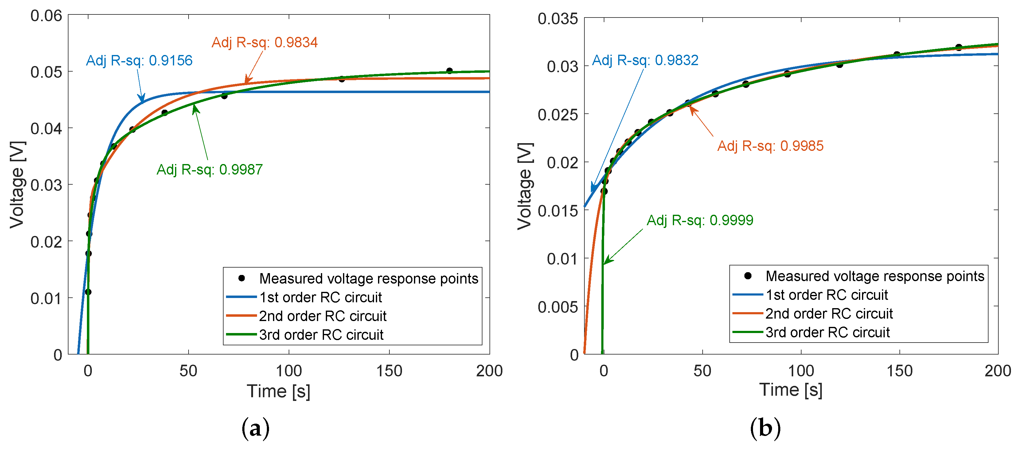
3.5. Voltage Response Circuit

The electrical elements in the model were tested while the battery underwent eight different C-rates at different S O C levels. The test procedure esd similar to the cte-OCV test, as shown in Figure 3, with the only difference being the amount of energy being charged/discharged in each step, and the resting time interval. In this test, the step size of charge/discharge was 0.15 Ah, and the relaxation time between each step was 3 min for both battery technologies. The resting time between charge/discharge was 1 h for both battery technologies.
The C-rates tested were: 0.05 C, 0.1 C, 0.15 C, 0.2 C, 0.25 C, 0.3 C, 0.4 C, and 0.5 C.

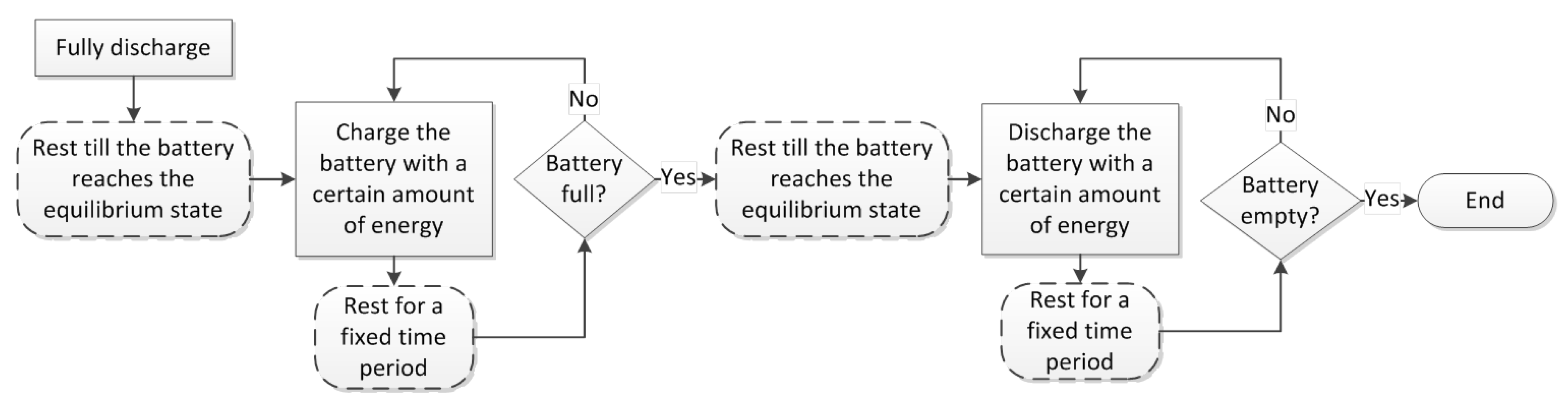
3.6. Parasitic Branch

A simplified measurement was applied to estimate the Coulombic efficiency in this study. The Coulombic efficiency was approximately measured and calculated from the integral recharge efficiency. The test procedure is outlined as follows.
  • Fully charge and discharge the battery to measure the initial battery capacity and the overall Coulombic efficiency.
  • Discharge the battery to a specific S O C value (x%) and note down the discharged capacity Q d .
  • Fully recharge the battery and record the recharged capacity Q c .
  • Calculate the recharge efficiency Q d / Q c assuming it is the averaged integral recharge efficiency at the mean S O C between x% and 100%.
  • Go back to Step 2 and repeat the steps until enough data points are obtained.
  • Test the whole procedure under different C-rates.
One thing should be noted: after each charge/discharge step, the battery needed to rest until reaching its equilibrium state, for 1 h in this case.
Then, the averaged integral recharge efficiency was fitted to Equation (10) to get the roughly estimated Coulombic efficiency as a function of S O C and C-rates.
The experimental settings are summarised in Table 2.

3.7. EECM Construction

After achieving all the required values of the electrical elements, the battery model can be constructed according to the EECM as shown in Figure 4.
It must be noted that the parasitic resistance R p shown in Figure 4 is not an actual circuit element in the EECM but only a notional lossy element that signifies side-reaction. In the proposed model in this study, the VRLA losses are actually quantified through the Coulombic efficiency, as shown in Equation (10).
The S O C of the battery can be represented by Equation (1), while the main branch current I m is calculated through Equation (11). The Coulombic efficiency η c is obtained from Equation (10).
I m = η c × I batt
The dynamic battery voltage of each part of the circuit can be calculated by using the achieved electrical elements through simple circuit analysis, as shown in Section 2.4. The battery voltage is shown in Equation (12).
V batt = V OC ± V o ± V s ± V l
where V batt is the battery voltage and the ± sign in Equation (12) is dependent on the current direction, i.e., + implies charging and − implies discharging the battery.

4. Results and Discussion

4.1. Experimental Results

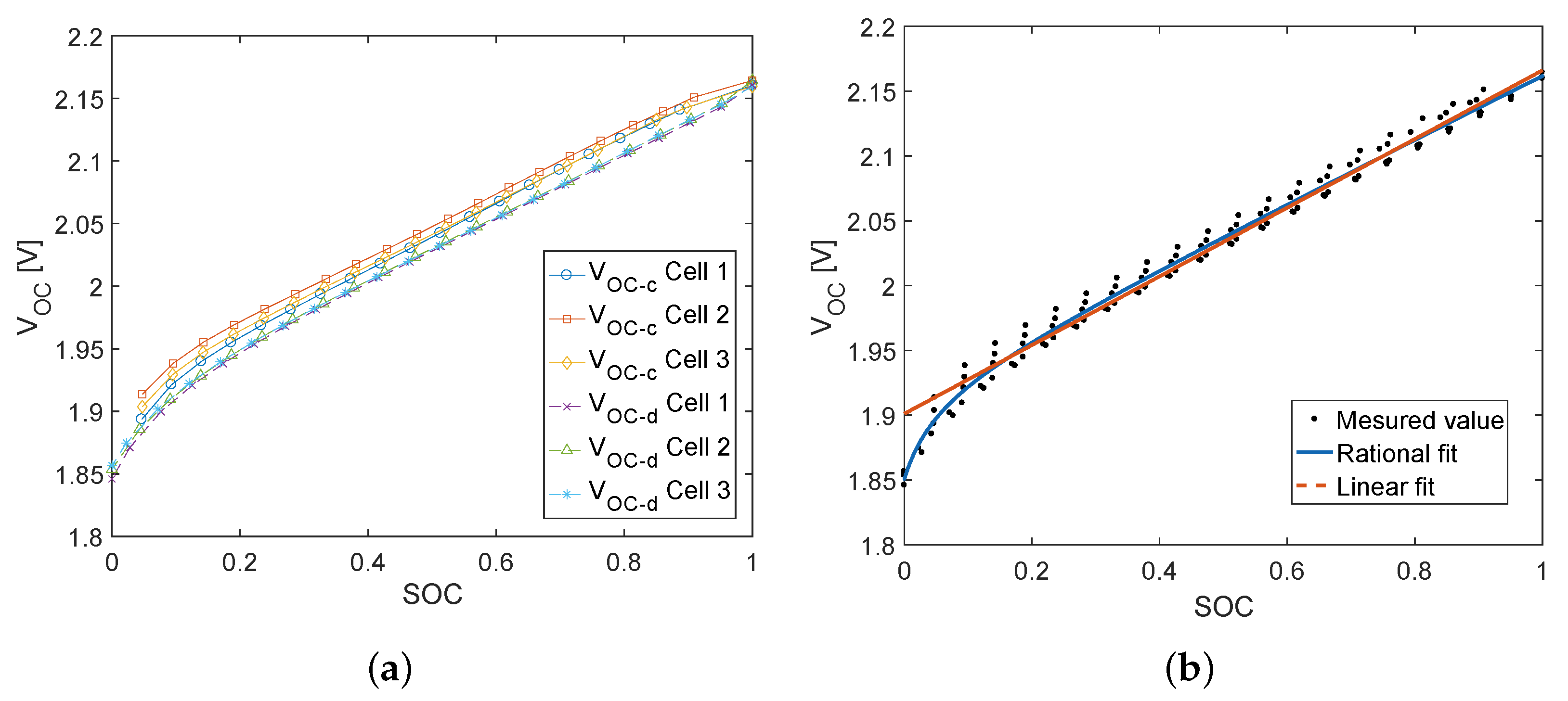
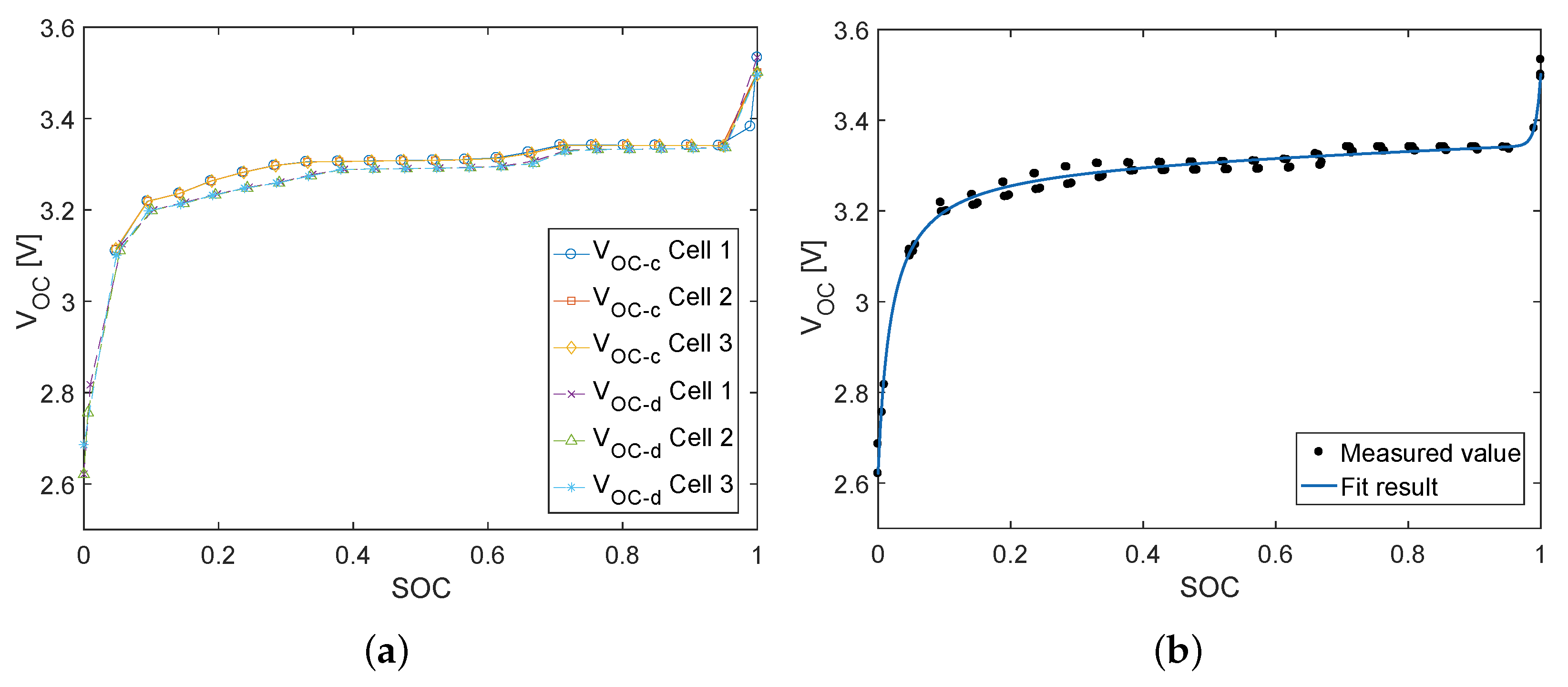
4.1.1. Cte-OCV as a Function of S O C

The cte-OCV and S O C are correlated; as the S O C increases, the cte-OCV also rises. Although many papers and manufacturer datasheets suggest that the cte-OCV of VRLA versus S O C shows a linear relation [33,34], our study found that a rational curve fit is better than a linear fit. This new fit is especially relevant when the battery is at low S O C , as plotted in Figure 5. Hence, the empirical-based rational Equation (13) was proposed and employed instead of a linear relationship.
V OC = 0.2428 × S O C 2 + 1.935 × S O C + 0.09876 S O C + 0.05336
In the case of LFP battery (Figure 6), there is a sudden increase in V OC when the S O C is close to 100%; similarly, the V OC drops when the S O C is almost 0%. The cte-OCV and S O C behaviour can be perfectly fitted into a double exponential curve [35]. This has been verified by this study, as shown in Figure 6, where the hysteresis phenomenon between the V OC values when charging or discharging is depicted. This hysteresis phenomenon was modelled in the electrical response circuit instead of V OC -SOC equation for both batteries.
The fitted cte-OCV-SOC result of LFP battery is written in Equation (14).
V OC = 3.307 × e 0.004117 S O C + 0.01772 + e 138.7 ( S O C 1.013 ) + 0.05098 × S O C

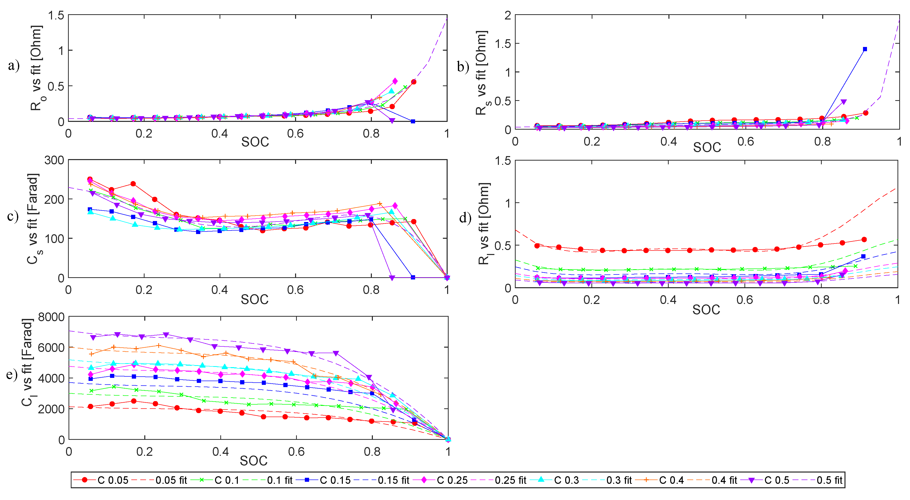
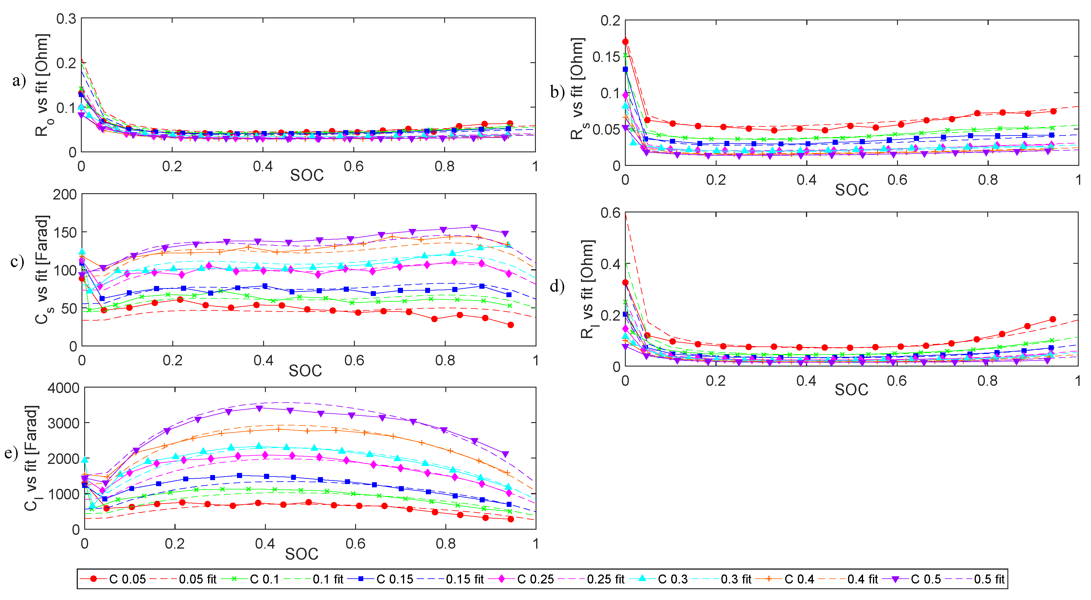
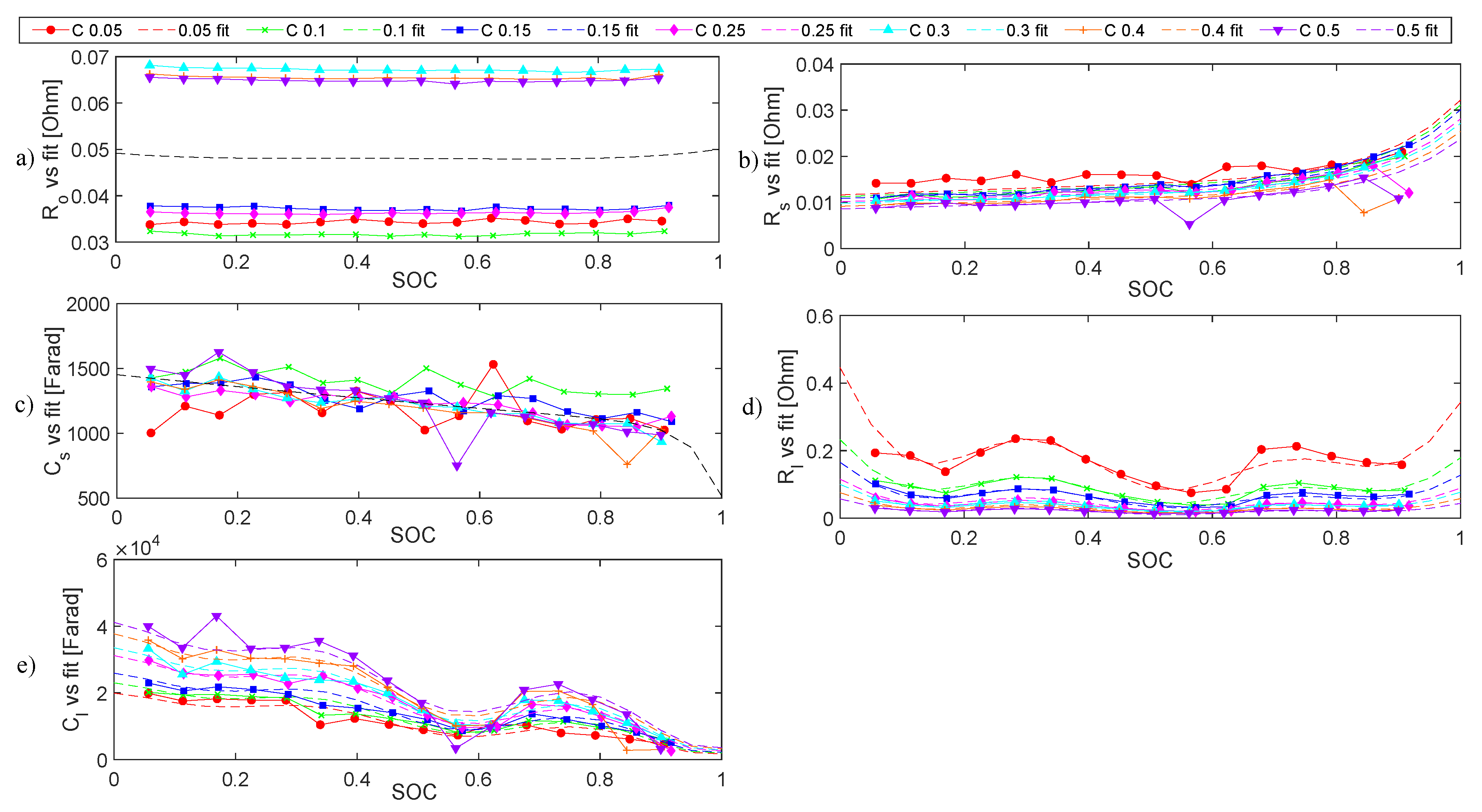
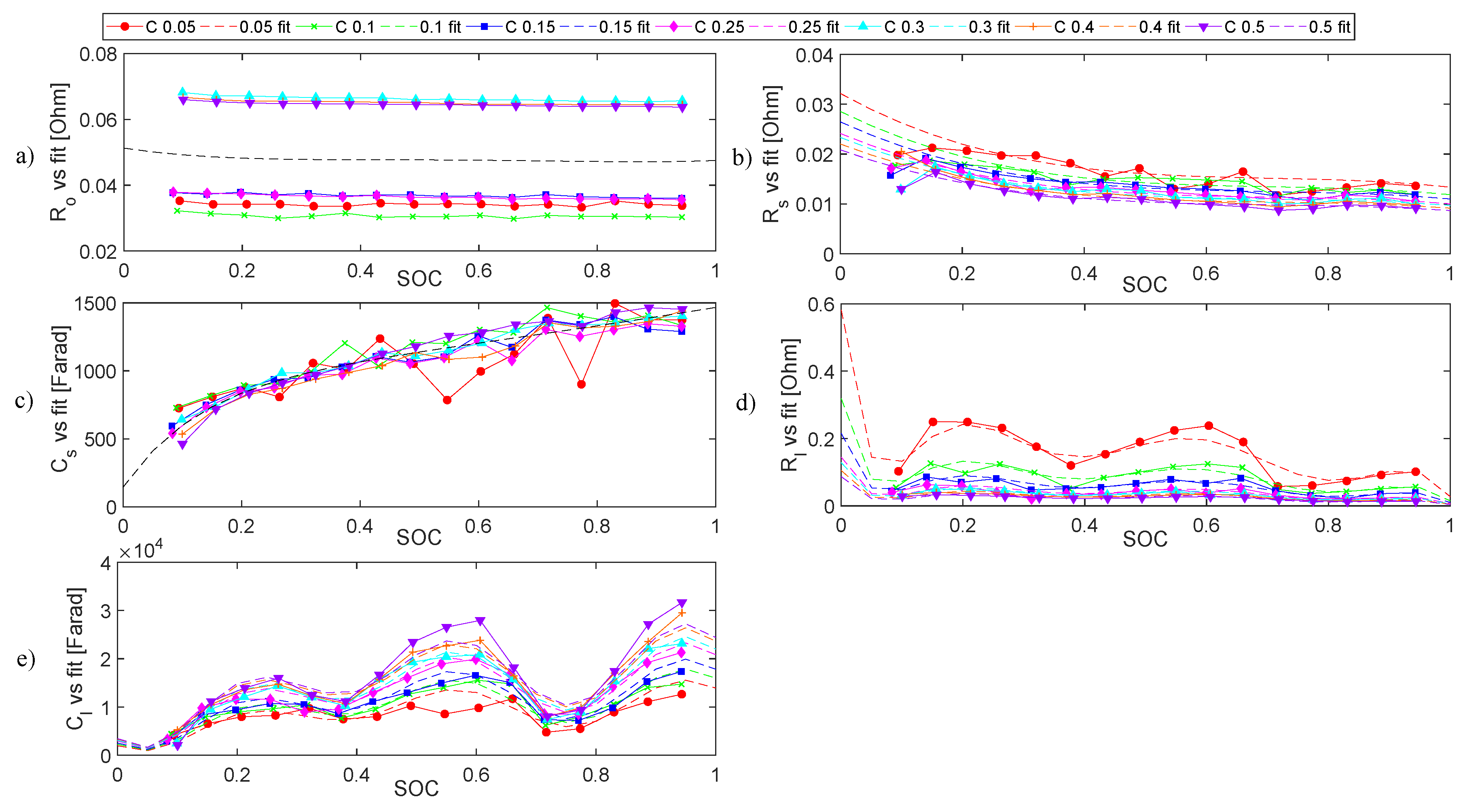
4.1.2. Internal Impedance

To choose an optimised EECM structure, the fitting comparison from first to third orders of RC circuits are plotted in Figure 7a,b. These two figures show one sample of voltage increase during the relaxation time and the fitting result with three different orders of RC circuits for both battery technologies.
From these curves, it can be concluded that the second order RC circuits have sufficient accuracy for both battery technologies. In addition, modelling the battery with a higher order of RC circuit requires more parameters. Thus, the second order RC circuits were selected for modelling both battery technologies owing to their lower complexity but sufficient accuracy.
The measured and fitted results of electrical elements in EECMs of LFP and VRLA batteries are shown in Figure 8, Figure 9, Figure 10 and Figure 11, where R o is the ohmic resistance; R s , C s are the values of RC pair representing the voltage relaxation in the short time-window ( τ 1 in Figure 2b); R l , C l are the values of RC pair used to represent the voltage relaxation in the long time-window ( τ 2 in Figure 2b).
In Figure 8 and Figure 9, some features of VRLA batteries can be inferred with respect to the internal impedance circuit elements, as listed below.
  • All the electrical elements show a strong dependency on S O C .
  • All the elements also show an inverse trend versus S O C in charge stage and discharge stage.
  • In terms of current dependency, elements during charge and discharge stages have diverse behaviours. While charging, only R l and C l values show a clear operational current dependence. While discharging, all the elements except R o are evidently influenced by the operational current.
Therefore, the R l and C l in discharge stage and all the elements in charge stage were modelled as the function of operational current. The detailed equations are listed as below:

Charge

R o _ VAc = 0.03782 · e 1.301 · S O C + 4.226 e 6 · e 12.64 · S O C
R s _ VAc = 4.246 e 13 · e 29.05 · S O C + 0.03787 · e 1.467 · S O C
C s _ VAc = 2666 · S O C 4 + 4113 · S O C 3 1558 · S O C 2 112.6 · S O C + 229.3
R l _ VAc = ( 4.952 · S O C 4 7.819 · S O C 3 + 4.168 · S O C 2 0.8406 · S O C + 0.1783 ) × 9.8198 e 4 · e 48.992 · C r 0.2 + 0.67172 · e 5.6015 · C r 0.2 + 0.3273 × 2.191 · S O C 3 + 2.62 · S O C 2 1.006 · S O C + 1.12
C l _ VAc = 8768 · S O C 1 3 1.961 e 4 · S O C 1 2 1.512 e 4 · S O C 1 × 11.66 · C r 0.2 3 4.366 · C r 0.2 2 + 2.43 · C r 0.2 + 1

Discharge

R o _ VAd = 0.01226 · S O C 3 + 0.007354 · S O C 2 + 0.02339 · S O C + 0.003575 S O C + 0.03138 × 78.342 · C r 0.2 4 + 25 · C r 0.2 3 + 4.6032 · C r 0.2 2 2.1016 · C r 0.2 + 1 × 0.4411 · e 16.19 · S O C + 0.9853 · e 0.01733 · S O C
R s _ VAd = 0.01341 · S O C 3 + 5.996 e 4 · S O C 2 + 0.02 · S O C + 6.888 e 4 S O C + 0.01043 × [ 6.6819 e 2 · e 0.0011936 · C r 0.2 + 0.15861 · e 14.305 · C r 0.2 667.3473 × 1.003 · e 0.01652 · S O C + 0.3767 · e 20.89 · S O C ]
C s _ VAd = 1116 · S O C 4 + 2320 · S O C 3 1640 · S O C 2 + 458.5 · S O C + 49.67 × 3.3295 · C r 0.2 2 + 2.7116 · C r 0.2 + 1 × 0.9504 · e 0.0464 · S O C + 0.3536 · e 609.2 · S O C
R l _ VAd = 0.1373 · S O C 4 0.1344 · S O C 3 + 0.04953 · S O C 2 + 0.01366 · S O C + 0.003415 S O C + 0.01673 × [ 0.13707 · e 16.624 · C r 0.2 1.021 · e 0.91595 · C r 0.2 + 1.8839 × 0.9371 · e 0.05663 · S O C + 0.421 · e 13.09 · S O C ]
C l _ VAd = 6879 · S O C 4 + 1.73 e 4 · S O C 3 1.877 e 4 · S O C 2 + 8425 · S O C + 492.4 × 3.8298 · C r 0.2 + 1 × 0.5753 · e 674 · S O C + 0.8458 · e 0.2202 · S O C
From the results in Figure 10 and Figure 11, some conclusions for LFP batteries can be drawn:
  • Except for R o , all other electrical elements show a strong dependency on SOC.
  • All electrical elements exhibit an inverse behaviour versus S O C in charge and discharge.
  • The operational current influences R s , R l and C l in both charge and discharge processes.
Therefore, all the elements could be expressed as the function of S O C for better accuracy, even though Ro does not vary too much with different S O C values. Elements R s , R l and C l were modelled as the function of both S O C and C-rate.
In these two figures, it can be observed that the fitting of all the electrical elements for battery model construction has a high accuracy. The equations of all these electrical elements for LFP battery are listed below.

Charge

R o _ LPc = 0.0334 · S O C 4 0.06141 · S O C 3 + 0.03985 · S O C 2 0.01104 · S O C + 0.04918
R s _ LPc = 0.01036 · e 0.295 · S O C + 3.829 e 6 · e 8.363 · S O C × 0.2304 · C r 2 0.775 · C r + 1.1458 × 0.2068 · S O C 2 + 0.1532 · S O C + 1.011
C s _ LPc = 1451 · e 0.3283 · S O C 9.562 e 8 · e 22.43 · S O C
R l _ LPc = [ 0.9515 + 0.05887 · c o s x w 0.06694 · s i n x w 0.01243 · c o s 2 x w 0.04918 · s i n 2 x w 0.02577 · c o s 3 x w 0.01927 · s i n 3 x w ] × 7.677 · e 28.9 · C r + 1.7054 · e 2.789 · C r × 0.1976 · S O C + 1.169 x = S O C ; w = 4.494
C l _ LPc = [ 1.672 e 4 + 7346 · c o s x w + 6107 · s i n x w + 3910 · c o s 2 x w + 859.6 · s i n 2 x w + 1356 · c o s 3 x w 4264 · s i n 3 x w ] × 1.272 · C r 2 + 2.346 · C r + 0.5817 × 0.08145 · S O C 2 + 0.06667 · S O C + 0.9769 x = S O C ; w = 4.76

Discharge

R o _ LPd = 0.04153 · S O C 4 0.09593 · S O C 3 + 0.07794 · S O C 2 0.0273 · S O C + 0.05125
R s _ LPd = 0.0325 · S O C 3 + 0.06854 · S O C 2 0.04985 · S O C + 0.02432 × 1.084 · e 0.534 · C r + 0.4643 · e 14.45 · C r × 0.03161 · S O C 2 0.07195 · S O C + 1.032
C s _ LPd = 909 · e 0.4785 · S O C 764.6 · e 7.692 · S O C
R l _ LPd = ( 219.3 · S O C 8 1031 · S O C 7 + 1986 · S O C 6 2021 · S O C 5 + 1167 · S O C 4 381 · S O C 3 + 65.8 · S O C 2 5.111 · S O C + 0.1754 ) × 1.307 · e 1.872 · C r + 6.3160 · e 20.67 · C r × 0.04198 · S O C + 0.9656
C l _ LPd = ( 1.22 e 4 2988 · c o s x w 2455 · s i n x w 1326 · c o s 2 x w 3567 · s i n 2 x w 5139 · c o s 3 x w 1171 · s i n 3 x w ) × 2.322 · C r 2 + 2.473 · C r + 0.5983 x = S O C ; w = 5.522

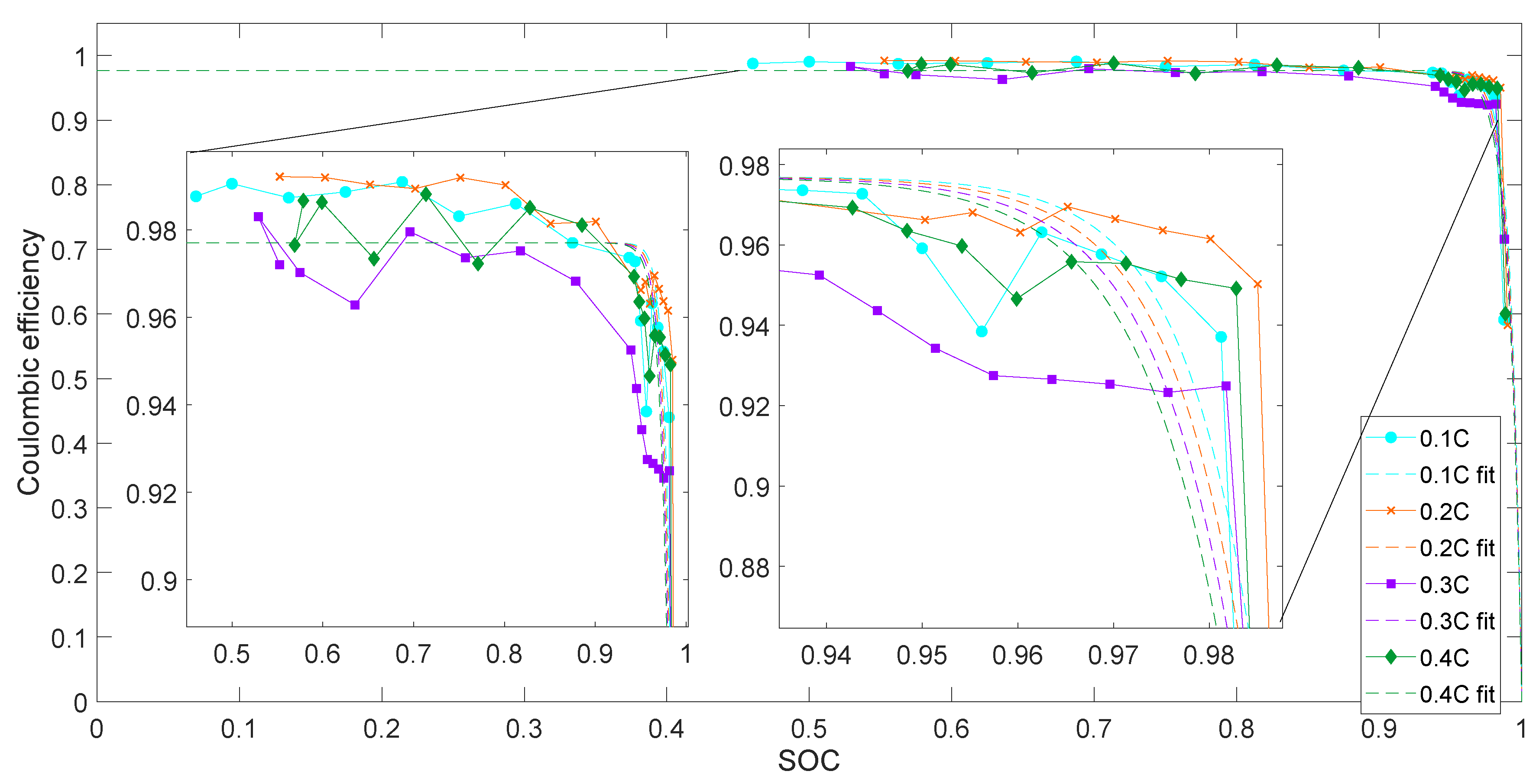
4.1.3. Coulombic Efficiency

The measured and fitted Coulombic efficiency result of VRLA battery is plotted in Figure 12.
The Coulombic efficiency is expected to decrease when current increases. However, the efficiency measured with 0.2C is higher than that measured with 0.1 C, and the result measured with 0.4 C is larger than the one measured with 0.3 C. This is because 0.1 C and 0.3 C measurements were operated on the same battery, while a different battery was tested with 0.2 C and 0.4 C. The differences between batteries may lead to this consequence. Nevertheless, the Coulombic efficiency tested with higher C-rate is lower than one tested with lower C-rate for the same battery. Therefore, the Coulombic efficiency is fitted into the modified Equation (10), which was introduced in Section 3.6. The result is shown in Equation (35).
η c = 0.977 1 e 5.466 5.569 e 3 C r 0.2 + 0.03745 × ( S O C 1 )
where C r is the C-rate.

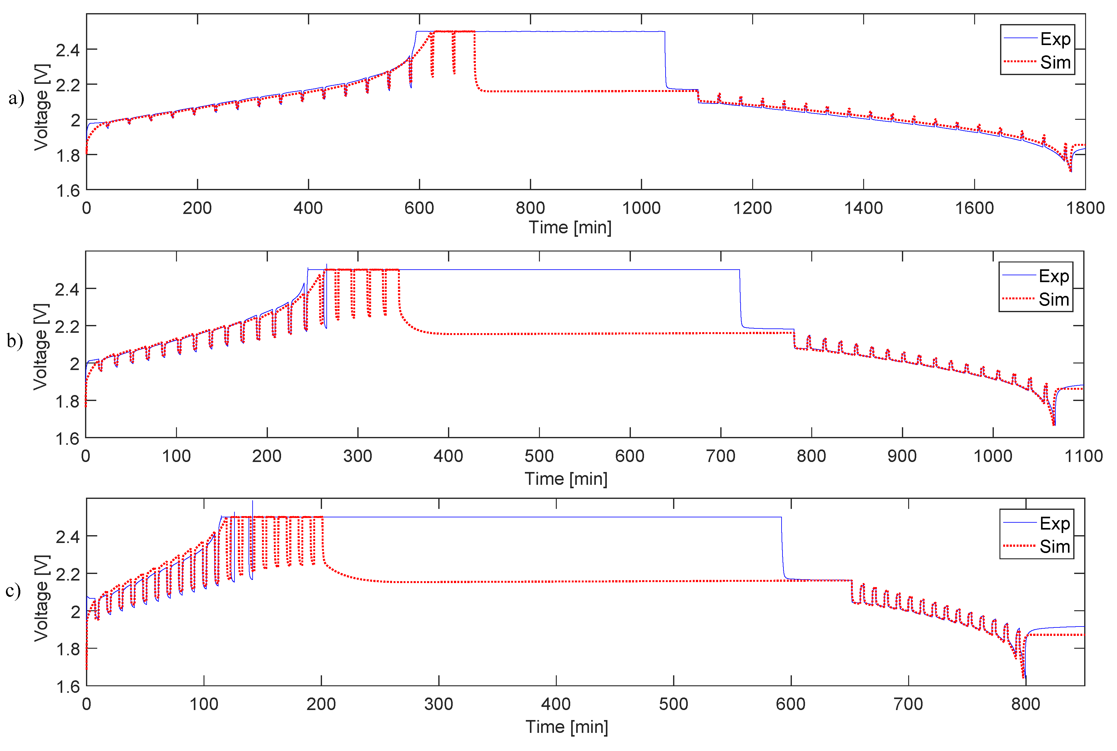
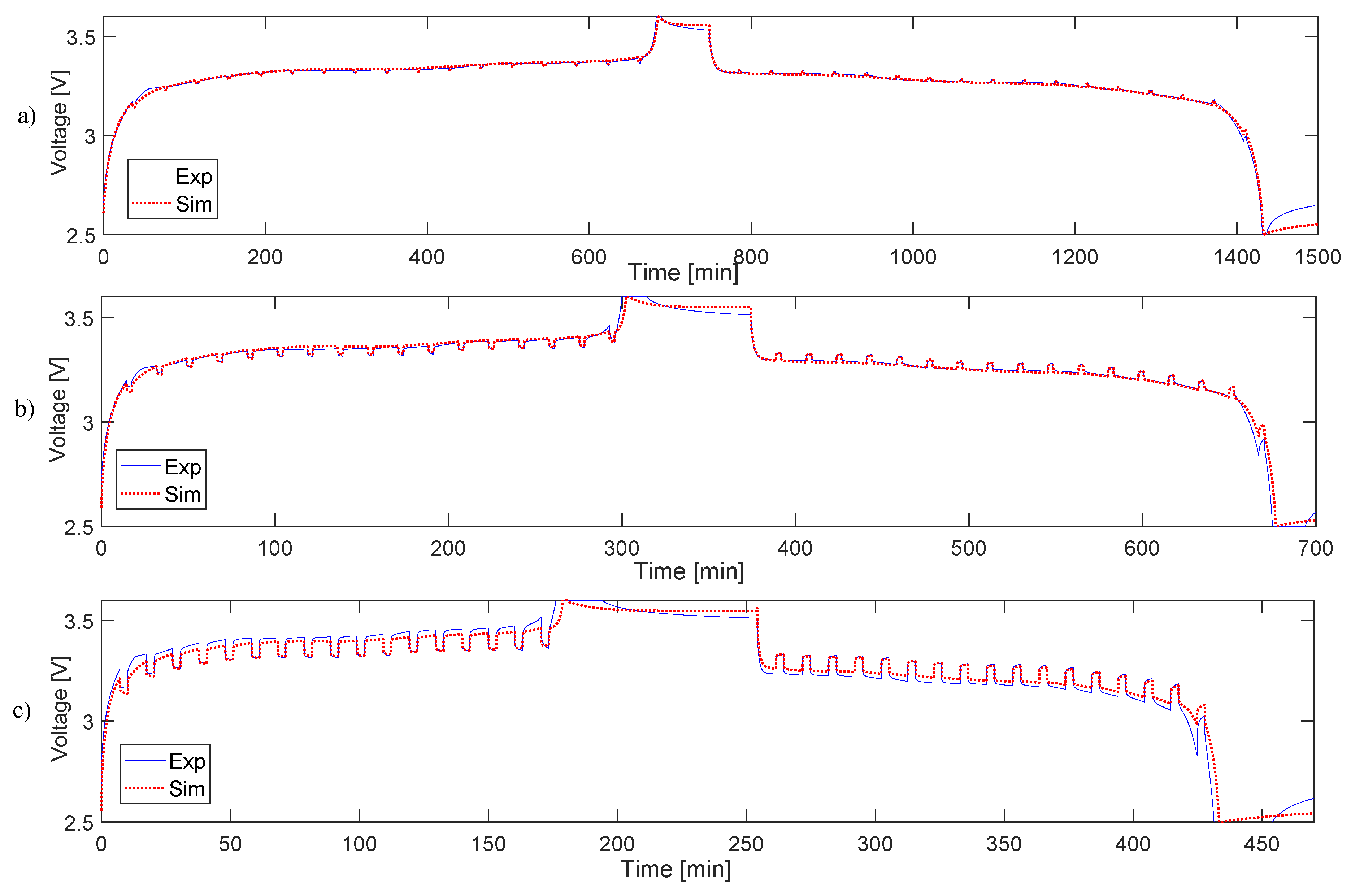
4.2. Simulation and Validation

In this section, the simulation results and the experimental data are compared. The comparison of measured voltage and simulated voltage for both battery technologies are plotted in Figure 13 and Figure 14.
As stated in Section 2.2, there are three essential features that should be reflected in the model: the storage feature, the voltage response and the parasitic side reaction. In this study, the S O C is the independent variable, and the voltage response is the main feature being modelled. The Coulombic efficiency is included in the storage circuit as well as the voltage response circuit. Hence, the voltage is selected to evaluate the accuracy of the model. To quantify the model accuracy, all the modelled and measured voltage values are calculated and evaluated using Equation (36). Then, for each battery, there is an averaged error value achieved among the whole charge/discharge process.
error = V sim V exp V exp × 100
where V sim is the simulated voltage and V exp is the measured voltage.
The constant voltage (CV) charging stages were omitted from the calculation because, in the real measurement, the pause steps are accomplished by the tester, and it depends on the natural battery features. This step counting outcome accomplished by the tester in CV stage is unable to be repeated with the simulation. How it works is reflected in Figure 13 and Figure 14. For example, the comparison results of VRLA batteries is shown in Figure 13. The discrepancy in this figure between the experimental and the simulation results (e.g., 600–1000, 250–700 and 150–650 min in Figure 13a–c, respectively) are due to the step counting method difference. Therefore, the CV stages for both battery technologies are eliminated.
The comparison results of VRLA batteries are in Figure 13. The simulated voltage curve increases slower than the measured one during the last charging stage before the battery reaches the CV stage, which is, e.g., around 600 min in Figure 13a. This slower increase trend of voltage is due to the modelled Coulombic efficiency loss. This can be attributed to the fact that the number of measured Coulombic efficiency data points when the S O C > 98% are insufficient. The fitted Coulombic efficiency result then cannot model the VRLA battery behaviour accurately when it reaches the high S O C stage, especially when the S O C higher than 98%.
For VRLA batteries, the maximum averaged error among all eight different C-rates is 1.7664%, while discounting the CV charging stage. The Coulombic efficiency fitting results might be one of the reason causing the error here.
Figure 14 shows the comparison results of LFP batteries. For LFP batteries, the maximum averaged error among all different C-rates, which is eight batteries in total, is 1.6708%. The discrepancy of the wedges shaped charge/discharge steps is mainly due to the differences in ohmic resistance. The error from ohmic resistance counts at least 0.5%.
The dynamic models of both battery technologies are therefore considered accurate.

5. Conclusions

In this study, two battery technologies (VRLA and LFP) were chosen for experimentally determining the dynamic behaviour of the battery, with the eventual goal of constructing an EECM model. The constructed model works well throughout the C-rate range from 0.05 C to 0.5 C, with an error lower than 2% for both LFP and VRLA batteries. The chosen C-rate range gave a better granularity for the intended application of SHS. The non-linear relation between S O C and V OC , the use of 2nd order RC circuit in EECM, and the quantification of the parasitic branch of VRLA cells in the form of S O C and C-rate based Coulombic efficiency η c were identified as methodological contributions for modelling the dynamic behaviour of VRLA batteries. Additionally, the model developed in this work is at the cell level, which is fully scalable to battery pack level. The proposed model can be used by SHS designers for understanding application-specific battery behaviour in the context of system design and analysis.

Recommendations and Future Work

Firstly, it is recommended to identify and develop a more accurate methodology to measure the Coulombic efficiency. The methodology presented in this paper is sufficient over most of the S O C range, except beyond 98%, where the achievable S O C granularity of the method is lower than desirable. Even though more accurate industrial test methods for Coulombic efficiency measurement are mostly chemical-based, it is still worthwhile developing a simple method with sufficient accuracy over the entire operational S O C range, especially for electrical models. Secondly, the batteries’ dynamic behaviour was modelled only when the batteries were new. The dynamic performance evolution through ageing is currently ignored. This is proposed to be improved in the future work. Thirdly, the impact of temperature needs to studied as an independent and controllable variable. Finally, this EECM is proposed to be applied in actual SHS use-cases by using battery charging and discharging profiles from SHS applications.

Author Contributions

Conceptualization, N.N. and J.P-G.; Methodology, Y.Y.; Validation, Y.Y. and N.N.; Formal Analysis, Y.Y. and N.N.; Investigation, Y.Y.; Resources, M.W., P.B., and M.Z.; Writing—Original Draft Preparation, Y.Y., N.N. and V.V-G.; Writing—Review and Editing, N.N., V.V-G., and Z.Q.; and Supervision, J.P-G., P.B. and M.Z.

Funding

This research received no external funding.

Acknowledgments

This work was supported by a fellowship from the Delft Global Initiative of the Delft University of Technology, the Netherlands. The authors thank Frans Oomes, Michel Steenvoorden from Storage of Electrochemical Energy group, Delft University of Technology for their timely help in the lab. The authors also thank Thomas van Dijk from E-stone batteries for allowing the use of the battery tester for some of the tests.

Conflicts of Interest

The authors declare no conflict of interest.

Nomenclature

V OC Open Circuit Voltage
SHSSolar home systems
Q t Battery actual capacity
VRLAValve Regulated Lead–Acid Battery
Q e Capacity that be extracted since the full battery stage
LFPLiFePO 4 Battery
I m Main branch current
I batt Battery current
SOCState of charge
EECMEquivalent Electrical Circuit Model
V batt Battery voltage
emfElectromotive Force
I p Side reaction Current
OCVOpen Circuit Voltage
C r C-rate
cte-OCVclose-to-equilibrium Open Circuit Voltage
Q n Nominal battery capacity
CC-CVConstant current-constant voltage charge/discharge scheme
R p Side reaction resistance
EODVEnd of discharge voltage
R o Ohmic resistance
V o Voltage response from Ohmic resistance
refReference
simSimulation
V interval Voltage response during the relaxation time
expExperiment
Q r Capacity that remaining in the battery
τ k Time interval in kth order circuit model
R k Resistance in kth order circuit model
C k Capacitance in kth order circuit model
V initial Initial voltage before relaxation
V k Voltage response in kth order circuit model
η c Coulombic efficiency
I test Test current
I ref Reference current
Q c / Q d Charged/discharged battery capacity
R s / R l Short/Long term resistance
C s / C l Short/Long term capacitance

References

  1. Organization for Economic Cooperation and Development, International Energy Agency. From Poverty to Prosperity, 1st ed.; IEA: Paris, France, 2017; p. 144. [Google Scholar]
  2. Narayan, N.; Papakosta, T.; Vega-Garita, V.; Qin, Z.; Popovic-Gerber, J.; Bauer, P.; Zeman, M. Estimating battery lifetimes in Solar Home System design using a practical modelling methodology. Appl. Energy 2018, 228, 1629–1639. [Google Scholar] [CrossRef]
  3. Leadbetter, J.; Swan, L.G. Selection of battery technology to support grid-integrated renewable electricity. J. Power Sources 2012, 216, 376–386. [Google Scholar] [CrossRef]
  4. Moseley, P.; Rand, D. The Valve-regulated Battery—A Paradigm Shift in Lead-Acid Technology. In Valve-Regulated Lead-Acid Batteries; Rand, D., Garche, J., Moseley, P., Parker, C., Eds.; Elsevier: Amsterdam, The Nederlands, 2004; Chapter 1; pp. 1–14. [Google Scholar]
  5. Hudak, N.S. 4-Nanostructured Electrode Materials for Lithium-Ion Batteries. In Lithium-Ion Batteries; Pistoia, G., Ed.; Elsevier: Amsterdam, The Nederlands, 2014; pp. 57–82. [Google Scholar]
  6. Nykvist, B.; Nilsson, M. Rapidly falling costs of battery packs for electric vehicles. Nat. Clim. Chang. 2015, 5, 329–332. [Google Scholar] [CrossRef] [Green Version]
  7. Zhang, C.; Li, K.; McLoone, S.; Yang, Z. Battery modelling methods for electric vehicles—A review. In Proceedings of the 2014 European Control Conference, Strasbourg, France, 24–27 June 2014; pp. 2673–2678. [Google Scholar]
  8. Mohanty, P.; Gujar, M. PV Component Selection for Off-Grid Applications. In Solar Photovoltaic System Applications: A Guidebook for Off-Grid Electrification; Mohanty, P., Muneer, T., Kolhe, M., Eds.; Springer International Publishing: Berlin, Germany, 2016; pp. 85–106. [Google Scholar]
  9. Deutsche Gesellshaft fur Sonnenenergie. Planning and Installing Photovoltaic Systems; Earthscan: London, UK, 2005; p. 304. [Google Scholar]
  10. Stroe, A.; Stroe, D.; Swierczynski, M.; Teodorescu, R.; Kær, S.K. Lithium-ion battery dynamic model for wide range of operating conditions. In Proceedings of the 2017 International Conference on Optimization of Electrical and Electronic Equipment (OPTIM) & 2017 International Aegean Conference on Electrical Machines and Power Electronics (ACEMP), Fundata, Romania, 25–27 May 2017; pp. 660–666. [Google Scholar]
  11. Liaw, B.Y.; Nagasubramanian, G.; Jungst, R.G.; Doughty, D.H. Modeling of lithium ion cells—A simple equivalent-circuit model approach. Solid State Ionics 2004, 175, 835–839. [Google Scholar]
  12. Tian, S.; Hong, M.; Ouyang, M. An experimental study and nonlinear modeling of discharge I-V behavior of valve-regulated lead-acid batteries. IEEE Trans. Energy Convers. 2009, 24, 452–458. [Google Scholar] [CrossRef]
  13. Pop, V.; Bergveld, H.J.; Danilov, D.; Regtien, P.P.; Notten, P.H. Introduction. In Battery Management Systems: Accurate State-of-Charge Indication for Battery-Powered Applications; Springer: Dordrecht, The Netherlands, 2008; pp. 1–9. [Google Scholar]
  14. Crompton, T. 1—Introduction to battery technology. In Battery Reference Book, 3rd ed.; Crompton, T., Ed.; Newnes: Oxford, UK, 2000; pp. 1–64. [Google Scholar]
  15. Vincent, C.A. 2–Theoretical background. In Modern Batteries, 2nd ed.; Vincent, C., Scrosati, B., Eds.; Butterworth-Heinemann: Oxford, UK, 1997; pp. 18–64. [Google Scholar]
  16. Dubarry, M.; Svoboda, V.; Hwu, R.; Yann Liaw, B. Incremental Capacity Analysis and Close-to-Equilibrium OCV Measurements to Quantify Capacity Fade in Commercial Rechargeable Lithium Batteries. Electrochem. Solid-State Lett. 2006, 9, A454–A457. [Google Scholar] [CrossRef]
  17. Root, M. The TAB Battery Book An In-Depth Guide to Construction, Design and Use; McGraw-Hill Companies: New York, NY, USA, 2010; p. 85. [Google Scholar]
  18. Doerffel, D. Testing and Characterisation of Large High-Energy Lithium-Ion Batteries for Electric and Hybrid Electric Vehicles. Ph.D. Thesis, University of Southampton, Southampton, UK, 2007. [Google Scholar]
  19. Waag, W.; Käbitz, S.; Sauer, D.U. Experimental investigation of the lithium-ion battery impedance characteristic at various conditions and aging states and its influence on the application. Appl. Energy 2013, 102, 885–897. [Google Scholar] [CrossRef]
  20. Lam, L.; Bauer, P.; Kelder, E. A practical circuit-based model for Li-ion battery cells in electric vehicle applications. In Proceedings of the 2011 IEEE 33rd International Telecommunications Energy Conference (INTELEC), Amsterdam, The Netherlands, 9–13 October 2011; pp. 1–9. [Google Scholar]
  21. Zhan, C.J.; Wu, X.; Kromlidis, S.; Ramachandaramurthy, V.; Barnes, M.; Jenkins, N.; Ruddell, A. Two electrical models of the lead–acid battery used in a dynamic voltage restorer. IEEE Proc. Gener. Trans. Distrib. 2003, 150, 175. [Google Scholar] [CrossRef]
  22. Ceraolo, M. New Dynamical Models of Lead—Acid Batteries. IEEE Trans. Power Syst. 2000, 15, 1184–1190. [Google Scholar] [CrossRef]
  23. Hu, X.; Li, S.; Peng, H. A comparative study of equivalent circuit models for Li-ion batteries. J. Power Sources 2012, 198, 359–367. [Google Scholar] [CrossRef]
  24. Panchal, S.; Mcgrory, J.; Kong, J.; Fraser, R.; Fowler, M.; Dincer, I.; Agelin-Chaab, M. Cycling degradation testing and analysis of a LiFePO4 battery at actual conditions. Int. J. Energy Res. 2017, 41, 2565–2575. [Google Scholar] [CrossRef]
  25. Jones, W.E.M.; Feder, D.O. Behavior of VRLA cells on long term float. II. The effects of temperature, voltage and catalysis on gas evolution and consequent water loss. In Proceedings of the Intelec’96—International Telecommunications Energy Conference, Boston, MA, USA, 6–10 October 1996; pp. 358–366. [Google Scholar]
  26. Buller, S. Impedance-based simulation models for energy storage devices in advanced automotive power systems. Ph.D. Thesis, RWTH Aachen University, Aachen, Germany, 2003. [Google Scholar]
  27. Kaushik, R.; Mawston, I.G. Coulombic efficiency of lead/acid batteries, particularly in remote-area power-supply (RAPS) systems. J. Power Sources 1991, 35, 377–383. [Google Scholar] [CrossRef]
  28. Andre, D.; Meiler, M.; Steiner, K.; Wimmer, C.; Soczka-Guth, T.; Sauer, D.U. Characterization of high-power lithium-ion batteries by electrochemical impedance spectroscopy. I. Experimental investigation. J. Power Sources 2011, 196, 5334–5341. [Google Scholar] [CrossRef]
  29. MACCOR. Series 4000 Automated Test System. Available online: http://www.maccor.com/ProductDocs/Data%20Sheet%20for%20Series%204000%20Test%20System.pdf (accessed on 10 August 2018).
  30. Enersys. Application Manual of CYCLONE AGM Single Cell. Available online: http://www.enersys-emea.com/reserve/pdf/EN-CYC-AM-007_1208.pdf (accessed on 10 August 2018).
  31. A123 Systems. Nanophosphate High Power Lithium Ion Cell ANR26650M1-B. Available online: https://www.batteryspace.com/prod-specs/6610.pdf (accessed on 10 August 2018).
  32. Yan, J.H.; Chen, H.Y.; Li, W.S.; Wang, C.I.; Zhan, Q.Y. A study on quick charging method for small VRLA batteries. J. Power Sources 2006, 158, 1047–1053. [Google Scholar] [CrossRef]
  33. Aylor, J.H.; Thieme, A.; Johnson, B.W. A Battery State-of-Charge Indicator for Electric Wheelchairs. IEEE Trans. Ind. Electron. 1992, 39, 398–409. [Google Scholar] [CrossRef]
  34. Pang, S.P.S.; Farrell, J.; Du, J.D.J.; Barth, M. Battery state-of-charge estimation. In Proceedings of the 2001 American Control Conference, Arlington, VA, USA, 25–27 June 2001; Volume 2, pp. 1644–1649. [Google Scholar]
  35. Hu, Y.; Yurkovich, S.; Guezennec, Y.; Yurkovich, B.J. Electro-thermal battery model identification for automotive applications. J. Power Sources 2011, 196, 449–457. [Google Scholar] [CrossRef]
Figure 1. Schematic of the overall EECM construction.
Energies 11 02305 g001
Figure 2. An example of voltage relaxation during rest interval in discharge with corresponding circuit elements. (a) The electrical circuit elements; (b) The voltage relaxation curve.
Energies 11 02305 g002
Figure 3. Test procedure of cte-OCV- S O C measurement and the Internal impedance circuit measurement.
Energies 11 02305 g003
Figure 4. The construction of the EECM. The subscripts s and l stand for short and long time duration respectively with respect to voltage relaxation ( τ 1 , τ 2 in Figure 2b).
Energies 11 02305 g004
Figure 5. Measured open circuit voltage versus S O C of VRLA battery: (a) V OC measured during charge and discharge separately; and (b) the measured data points and the fitted curves.
Energies 11 02305 g005
Figure 6. Measured open circuit voltage versus S O C of LFP battery: (a) the hysteresis of V OC when charge and discharge the battery separately; (b) the measured data points and the fitted curve.
Energies 11 02305 g006
Figure 7. Comparison of accuracy with modelling battery into different orders of RC circuits: (a) VRLA battery; (b) LFP battery.
Energies 11 02305 g007
Figure 8. The values of RC elements and their fitted results: VRLA batteries during charge.
Energies 11 02305 g008
Figure 9. The values of RC elements and their fitted results: VRLA batteries during discharge.
Energies 11 02305 g009
Figure 10. The values of RC elements and their fitted results: LFP batteries during charge.
Energies 11 02305 g010
Figure 11. The values of RC elements and their fitted results: LFP batteries during discharge.
Energies 11 02305 g011
Figure 12. Measured Coulombic efficiency of VRLA battery with SOC and with different C-rate.
Energies 11 02305 g012
Figure 13. Comparison of experimental result and simulation result-VRLA battery: (a) test with 0.1 C; (b) test with 0.25 C; and (c) test with 0.5 C.
Energies 11 02305 g013
Figure 14. Comparison of experimental result and simulation result-LFP battery: (a) test with 0.1 C; (b) test with 0.25 C; and (c) test with 0.5 C.
Energies 11 02305 g014
Table 1. Specification and summarized charge/discharge method for both battery technologies.
Battery BrandA123systems® APR26650M1BCyclon® AGM D Single Cell
Battery capacity2.5 Ah2.5 Ah
Nominal voltage3.3 V2 V
End of chargeCC-CV: 3.6V until I ≤ 0.01CCC-CV: 2.5V until I ≤ 0.002 C
End of dischargeCC-CV: 2.5V until I ≤ 0.01 CDepending on C-rate and EODV:
C-rate0.050.10.20.412>5
EODV1.751.71.671.651.61.551.5
Table 2. Experimental setting for Coulombic efficiency measurement for VRLA battery.
High SOC Low SOC
SOC value90% to 99%; 1% steps10% to 90%; 10% steps
C-rate0.1 C, 0.2 C, 0.3 C, 0.4 C0.1 C, 0.2 C, 0.3 C, 0.4 C

